Rotation periods for very low mass stars in the Pleiades

We present the results of a photometric monitoring campaign for very low mass (VLM) members of the Pleiades. Periodic photometric variability was detected for nine VLM stars with masses between 0.08 and 0.25 $M_{\odot}$. These variations are most likely caused by co-rotating, magnetically induced spots. In comparison with solar-mass stars, the photometric amplitudes are very low ($<0.04$ mag), implying that either the fraction of the spot-covered area, the asymmetry of the spot distribution, or the contrast between spots and photospheric environment decreases with mass. From our lightcurves, there is evidence for temporal evolution of the spot patterns on timescales of about two weeks. The rotation periods range from 2.9 h to 40 h and tend to increase linearly with mass. Compared with more massive stars, we clearly see a lack of slow rotators among VLM objects. The rotational evolution of VLM stars is investigated by evolving the previously published periods for very young objects (Scholz & Eislöffel se04 (2004)) forward in time, and comparing them with those observed here in the Pleiades. We find that the combination of spin-up by pre-main sequence contraction and exponential angular momentum loss through stellar winds is able to reproduce the observed period distribution in the Pleiades. This result may be explained as a consequence of convective, small-scale magnetic fields.

1 Introduction

Rotation is a key parameter of stellar evolution. The investigation of the rotational evolution of solar-mass stars showed that the angular momentum regulation is directly connected to basic stellar physics: Solar-mass stars rotate slowly in the T Tauri phase, probably because of rotational braking through magnetic coupling between star and disk. After loosing the disk, the rotation accelerates as the stars contract towards the zero age main sequence (ZAMS). From here, the rotation rates decrease again as a consequence of angular momentum loss through stellar winds (Bouvier et al. bfa97 (1997), Bodenheimer b95 (1995) and references herein; see also the recent reviews of Stassun & Terndrup st03 (2003) and Mathieu m03 (2003)). Main ingredients for models of rotational evolution are thus angular momentum loss via a) magnetic interaction between star and disk and b) stellar winds.

One of the cornerstones of our understanding of rotational evolution are the rotation rates for Pleiades members, since the age of the Pleiades (125 Myr, Stauffer et al. ssk98 (1998)) marks the beginning of the main sequence for solar-mass stars, and thus the turning point in their angular momentum evolution. From the work of Magnitskii (m87 (1987)), Stauffer et al. (ssb87 (1987)), van Leeuwen et al. (lam87 (1987)), Prosser et al. (1993a , 1993b , psd95 (1995)), and Krishnamurthi et al. (ktp98 (1998)), we have a large number of photometric rotation periods for Pleiades stars with $0.5<M<1.2\,M_{\odot}$ in hand, available from the Open Cluster Database compiled by C.F. Prosser and J.R. Stauffer. For very low mass (VLM) stars with $M<0.4\,M_{\odot}$, however, there are only two periods known (Terndrup et al. tkp99 (1999)). First insights into the rotational behaviour of the VLM members of the Pleiades come from rotational velocity studies (Terndrup et al. tsp00 (2000) and references herein), indicating a lack of slow rotators among VLM stars. This has been explained by a mass-dependent saturation threshold of the angular momentum loss rate (e.g., Barnes & Sofia bs96 (1996), Krishnamurthi et al. kpb97 (1997)).

Whereas the rotational velocity analysis suffers from projection effects and high uncertainties, rotation periods can be determined from photometric lightcurves without ambiguity with respect to the inclination angle and with high precision. Considering the lack of known rotation periods for VLM objects, it is necessary to compile a period database that complements the known periods for solar-mass stars. This was the main motivation for our long-term project dedicated to the study of rotation periods in the VLM regime. In the first publication of this project, we presented 23 rotation periods for VLM objects in the very young cluster around $\sigma$ Ori (Scholz & Eislöffel se04 (2004), hereafter SE2004), giving us the first, although rough approximation for the initial period distribution of VLM objects. Here we report the discovery of nine new rotation periods for VLM stars in the Pleiades, increasing the VLM period sample for this cluster by a factor of 4.5. With the periods from the $\sigma$ Ori cluster and the Pleiades, we are now able to set contraints on the angular momentum regulation in VLM objects during the first $10^{8}$ years of their evolution.

The paper is structured as follows: In Sect. 2, we outline the selection of our targets, the time series observations, the image reduction, and the photometry. We then report about the time series analysis in Sect. 3. In Sect. 4, we discuss the origin of the observed photometric variability. Subsequently, in Sect. 5, we investigate the mass dependence of the Pleiades periods, by comparing our data with periods for solar-mass stars and $v\sin i$ measurements. Then, we try to reconstruct the VLM period distribution in the Pleiades from our periods for younger objects, taking into account basic angular momentum regulation mechanisms in Sect. 6. Finally, we present our conclusions in Sect. 7.

2 Targets, observations, data reduction

The Pleiades are a preferred hunting ground for Brown Dwarfs and VLM stars. Here, the first cluster Brown Dwarfs at all were detected (Rebolo et al. rzm95 (1995), rmb96 (1996)). In the last decade, a number of deep, large surveys explored the mass function of this cluster well down into the substellar regime (e.g., Moraux et al. mbs03 (2003), Adams et al. asm01 (2001), Bouvier et al. bsm98 (1998)). Our target sample is based on the survey of Pinfield et al. (phj00 (2000), pdj03 (2003)), which covers six square-degrees and is complete down to $I_{C}=19.6$, corresponding to a mass of roughly 0.05 $M_{\odot}$ (Baraffe et al. bca98 (1998)). By the time of our observations, this was the largest and deepest object sample available. Pinfield et al. (phj00 (2000)) observed in the I- and Z-band for the primary photometric identification of their candidates. Contaminating field stars were rejected based on near-infrared photometry and proper motions. Their cluster member list comprises 339 objects, including 30 Brown Dwarfs. This survey confirms numerous cluster member candidates from other studies.

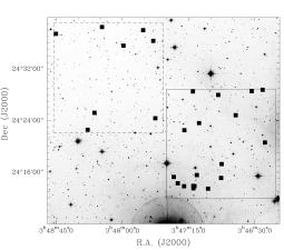
Figure 1: Time series fields in the Pleiades: The image shows our two fields (field A - solid lines, field B - dashed lines) plotted over a DSS image. The squares mark our targets, which are Pleiades members from the survey of Pinfield et al. (phj00 (2000)).

A subsample of the Pinfield et al. list serves as targets for our photometric monitoring campaign. We used the CCD camera at the 1.23-m telescope on Calar Alto, which has a field of view of $17^{\prime}\times 17^{\prime}$ and a pixel scale of 0$\aas@@fstack{\prime\prime}$5/pix. All time series images were taken in the I-band and with 600 s exposure time. To increase the number of targets, we decided to observe two fields. These two fields were selected by maximising the number of cluster members on the detector area. Both fields together contain 39 Pleiades members with masses up to $0.5\,M_{\odot}$. Of these, 13 are too bright and hence saturated on our deep images. The remaining 26 targets have masses between 0.06 and 0.25$\,M_{\odot}$. The positions of our fields and these 26 candidates are shown in Fig. 1.

Our time series covers 18 nights from 2. to 19. October 2002. Observations were possible in 15 nights within this time span, and in seven nights we were able to obtain more than 10 images per field. The sampling is thus quite dense (see Fig. 2). In 10 nights, both fields were monitored alternately. The remaining 4 observing nights were used to increase our sensitivity for very short periods by concentrating mainly on one field (i.e. 2 nights for each). Therefore, the sampling is slightly different for the two fields.

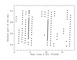
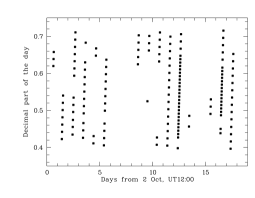
Figure 2: Observing data distribution for the time series campaign in field A (upper panel) and field B (lower panel). Plotted is the non-integer fraction of the observing time against the observing time.

The reduction of the time series images included bias subtraction, flatfield correction, and fringe removal (see SE2004 for details). For the further processing, we used the difference image analysis package of the ’Wendelstein Calar Alto Pixellensing Project’ (see Riffeser et al. rfg01 (2001), Gössl & Riffeser gr02 (2002)), which is based on ’Optimal Image Subtraction’ (Alard & Lupton al98 (1998)). This package is particularly well-suited for CCD image from the Calar Alto 1.23-m telescope and improves the photometric precision by several mmag compared with PSF fitting photometry, as we have demonstrated in SE2004.

The result of the ’Optimal Image Subtraction’ pipeline are difference images which contain only photon noise and variable sources. On these frames, we performed aperture photometry for all objects. A catalogue of the pixel positions of all objects was determined previously using SExtractor (Bertin & Arnouts ba96 (1996)) on a stacked image. By dividing the fluxes from the difference image through the fluxes from the stacked image, we calculated relative fluxes for all objects in all frames. These relative fluxes were then transformed to relative magnitudes with $m_{rel}=-2.5\log_{10}(1+f_{\mathrm{rel}})$. We determined the photometric precision of our photometry by calculating mean and rms of all lightcurves, after excluding 3$\sigma$ outliers. Similar to our result in SE2004, we achieve a precision of 4 mmag for the brightest targets.

3 Time series analysis

For the time series analysis, we used the procedures described in SE2004. In a first step, the lightcurve of each target was inspected visually. We find no signs of sudden brightness eruptions (like flares). The following lightcurve analysis is described in the next two subsections.

3.1 Generic variability test

To examine the photometric variability of our VLM Pleiades members, we analysed the scatter in their lightcurves. To increase the sensitivity, this test was done after binning the lightcurves by a factor of four, i.e. we averaged the relative magnitudes over two hours observing time. In Fig. 3, we plot the rms of all candidate lightcurves $\sigma_{cand}$ after excluding $\geq 3\sigma$ outliers. The solid line in Fig. 3 was determined by fitting the rms of the lightcurves of all stars in both fields with a low degree polynomial. Thus, this function gives us an estimate for the average rms of the lightcurves of nonvariable stars ($\sigma_{av}$). Using the statistical F-test, we compared the rms of each candidate lightcurve $\sigma_{cand}$ with $\sigma_{av}$ for the respective brightness. All variable objects on the significance level of 99% are marked with a cross. Out of 26 VLM members of the Pleiades, 12 (46%) are variable according to this criterion. The amplitudes of the variability are below 2% in all cases. This result shows that VLM objects in the Pleiades exhibit photometric variability, but to a very low degree. We find no large amplitude variability, as detected for similar mass objects in the much younger cluster around $\sigma$ Ori (SE2004). This is not surprising, since the large amplitude variations there are probably caused by accretion processes, which are not expected for the older objects in the Pleiades.

For eight of the twelve variable objects, we found significant periodic variability (see Sect. 3.2). These objects will be discussed in the following Section. The remaining four targets clearly show anomalies in their lightcurves. The lightcurves of objects BPL111 and BPL128 (catalogue number of Pinfield et al. phj00 (2000)) show noticeable variability only in part of the time series data. For BPL111, the mean relative magnitude deviates in the last two nights by $-0.015$ mag (night 17) and $+0.03$ mag (night 18) from the average of the whole time series. For object BPL128, the variation is increased by 30% in the second third of the lightcurve compared to the remaining data points. The behaviour of these two objects is most likely caused by evolving surface properties, and will be discussed in Sect. 4. The lightcurves of the objects BPL130 and BPL177 exhibit several single data points which lie $2\ldots 3\sigma$ above or below the average. Excluding these data points, the objects appear to be non-variable. The nature of these outliers remains unclear, and has to be verified by monitoring with better time resolution.

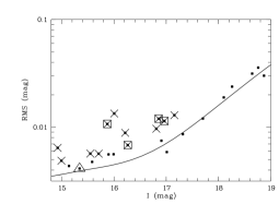
Figure 3: Lightcurve rms vs. magnitude for all targets: The solid line shows our photometric precision, determined by fitting the rms of all stars in our fields with a low degree polynomial. The VLM Pleiades members are shown as dots, and all variable objects among them are marked with a cross. The four objects, which are variable but without periodicity are additonally marked with a square. One object with significant periodic variability, but without variability detection in the generic test, is marked with a triangle (object BPL150, see Sect. 3.2). The magnitudes on the x-axis are instrumental, though the deviations from the I-band magnitudes given by Pinfield et al. (phj00 (2000)) are $\leq 0.3$ mag.

3.2 Period search

Our period search is based on the Scargle periodogram (Scargle s82 (1982)). It includes a sequence of tests to control the significance of a detected periodicity and to assure that the period is intrinsic to the target. Furthermore, it uses the CLEAN algorithm (Roberts et al. rld87 (1987)) to distinguish between real periodogram peaks and artifacts. The period search procedure requires that five criteria are fulfilled:

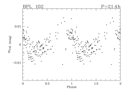
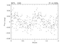
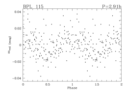
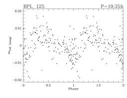
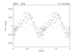
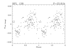
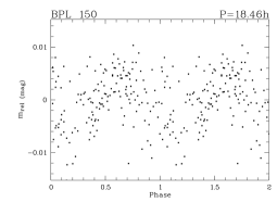
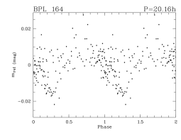
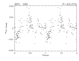
Figure 4: Phased lightcurves for the detected periodicities. No. and period from Table 1 are indicated.

a) The Scargle periodogram shows a peak exceeding the 99% significance level, as given by Horne & Baliunas (hb86 (1986)). This gives us a first estimate for the False Alarm Probability (FAP) of the period.

b) The period is confirmed by the CLEAN algorithm, i.e. the highest peak in the CLEANed periodogram corresponds to the detected period. This assures that the period is not due to sidelobes and aliases, caused by the window function of the data.

c) The scatter in the lightcurve is significantly reduced after the subtraction of the (sine-wave approximated) period. (For the comparison of the scatter we used the statistical F-test.)

d) Periodogram and phased lightcurve of at least ten nearby reference stars do not show the same period as the candidate. This makes sure that the detected period is an intrinsic property of the candidate lightcurve.

e) The periodicity is visible in the phased lightcurve. We note that this last test is the only subjective test among our period search criteria. It has to be treated with caution, because our time series are composed of 150 or more data points. This large number of data points enables a reliable period detection, even if the noise level is very high (see Sect. 3.3).

Table 1: Candidates with significant periodic variability (see text for explanations).

BPL	M($M_{\odot}$)	P(h)	$\Delta$P(h)	A(mag)	FAPE(%)	N
102	0.25	21.4	0.49	0.013	$<0.01$	158
106	0.08	4.08	0.02	0.032	$<0.01$	159
115	0.10	2.91	0.01	0.014	$0.01$	160
125	0.15	19.35	0.34	0.012	$<0.01$	159
129	0.13	9.64	0.10	0.034	$<0.01$	160
138	0.25	25.81	0.58	0.015	$<0.01$	159
150	0.18	18.46	0.32	0.008	$0.02$	152
164	0.13	20.16	0.53	0.021	$<0.01$	150
190	0.15	40.27	1.57	0.012	$<0.01$	153

The final FAPs for the periods were determined using the bootstrap approach following Kürster et al. (ksc97 (1997)). For each candidate, we generated 10000 randomized lightcurves by retaining the observing times and randomly redistributing the observed relative magnitudes amongst the observing times. The Scargle periodogram was calculated for each of these randomized datasets, and the power of the highest peak was recorded in each of them. The FAP is the fraction of datasets for which the power of the highest peak exceeds the power of the periodicity in the observed lightcurve. It turned out that these empirical values for the FAP are very similar to our first FAP estimate from the peak height in the Scargle periodogram. We accepted a period if the FAP is below 1%. For a more detailed discussion of the validity of the bootstrap approach, we refer to SE2004.

We established periodic variability for nine targets. Eight of these objects are also variable according to the generic variability test in Sect. 3.1). The period search is more sensitive than the simple variability test of Sect. 3.1, therefore it detects one more low amplitude variable (object BPL150). The periods range from 3 to 40 hours, the amplitudes from 0.01 to 0.03 mag. In Table 1, we list all relevant data for these objects. The first column gives the object no. according to the nomenclature of Pinfield et al. (phj00 (2000)). Our periods were determined by fitting the CLEANed periodogram peak with a Gaussian. Period errors ($\Delta$P) are based on the half width at half maximum of the fitted Gaussian, transformed to time space. The amplitudes (A) correspond to the peak-to-peak-range of the binned lightcurve. N is the number of data points used for the period search. The masses in column 2 are estimated by transforming the $I_{KP}$-band magnitudes of Pinfield et al. (phj00 (2000)) in the $I_{C}$ band, using the transformation given in Pinfield et al. (phj00 (2000)). These magnitudes were then compared with the Pleiades evolutionary tracks of Baraffe et al. (bca98 (1998)), adopting $m-M=5.5$ and an age of 125 Myr. The phased lightcurves of all objects with detected period are shown in Fig. 4.

For several objects with significant periodic variability, the phased lightcurve of Fig. 4 shows a relatively high noise level. As noted above, this does not necessarily mean that the period detection is not reliable, because of our large number of data points. However, it could be an indication for the evolution of surface properties. If the surface pattern is constant, the amplitude of the periodic signal will be constant. On the other hand, if the surface pattern evolves, the amplitude of the periodicity may vary.

To investigate the surface pattern stability, we examined the phased lightcurves of the periodic objects for parts of the time series. Five out of nine objects, namely the targets 106, 115, 164, 150, 190, show clear evidence for spot evolution in the course of our 18-night observing run. For these objects, the period is obvious in the first or last part of the time series, but relatively noisy over the whole dataset. In Fig. 5, we show exemplarily the phased lightcurves for objects 115 and 150 for a part of the time series. In both cases, the period is much more evident than in Fig. 4.

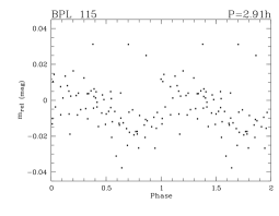
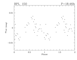
Figure 5: Phased lightcurves for part of the time series of objects 115 (upper panel, only datapoints after 10 Oct UT12:00) and 150 (lower panel, only datapoints before 6 Oct UT12:00)

.

3.3 Sensitivity

From our time sampling (see Fig. 2), we estimate that we are sensitive to periods from 0.5 hours up to 18 days. To assess the sensitivity of our period search more precisely, we executed simulations similar to those described in SE2004. We selected non-variable objects from our data and added sine-shaped periodicities to their lightcurves, so that the signal-to-noise ratio (defined as ratio of period amplitude and scatter in the original lightcurve) is similar to the periodicities in Table 1. We computed the Scargle periodogram for periods between 0.01 h and 300 h and recorded the frequency of the highest peak. The absolute difference between the imposed period and the detected period serves as an indicator for the reliability of our period search. Since the sampling is slightly different for both fields, we did the simulation for both fields separately. The results are shown in Fig. 6. The reliability of the period search is slightly variable, but the uncertainty is below 10% up to periods of 300 h, with two exceptions: a) In both diagrams, there is a small peak at one day, caused by the regular gaps between the observing nights, and b) for field A, there is a narrow window of non-sensitivity between periods of 240 and 270 h. This can be explained with the lack of data points between days 6 and 11 in Fig. 2 (lower panel).

From this simulation, we can be confident that we are sensitive to photometric periods between 0.01 h and 300 h, with no major biases. For longer periods, the uncertainty of the period determination generally increases, and there is a large gap of non-sensitivity for field A around periods of 320 h, probably caused by the lack of data points between days 13 and 17 in Fig. 2 (upper panel). Therefore, the period search might be not sensitive for $P>300$ h. Since we do not observe any period between 50 h and 235 h, a range where our period search is reliable within $\pm 10$%, it is, however, very unlikely that there exist many periods $>300$ h in our lightcurves.

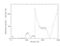
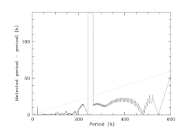
Figure 6: Sensitivity of the period search: The absolute difference between detected period and true period vs. true period for field A (upper panel) and field B (lower panel). The signal-to-noise ratio of the periodicity is 2.5; the dotted line corresponds to a period error of 10%.

Furthermore, we investigated the sensitivity of our period search as a function of signal-to-noise ratio. This time, we fixed the period to $P=18$ h, a value typical for our detected periodicities, and varied the amplitude of the added sine wave. Again, we computed the Scargle periodogram and recorded the frequency of the highest peak. The difference between imposed period and detected period is larger than 10 h for very small amplitudes, but decreases to values $<0.04$ h for signal-to-noise $>1.05$. Thus, our period search is sensitive down to signal-to-noise ratios of about 1.05. On the other hand, the minimum signal-to-noise ratio of our periods in Table 1 is 1.27 (object BPL115), making us confident that our periods are reliable.

4 Origin of the observed variability

Following the usual interpretation, we attribute the observed periodic variability in the lightcurves to the existence of surface features co-rotating with the objects, which must be asymmetrically distributed to induce a photometric variation. The surface features could arise from two fundamentally different processes, dust condensation and magnetic activity, which will be discussed in the following.

Recently, several groups reported about photometric variability of ’ultracool dwarfs’ in the field, i.e. VLM objects with spectral types L or T (Tinney & Tolley tt99 (1999), Bailer-Jones & Mundt bm01 (2001), Martín et al. mzl01 (2001), Clarke et al. cot02 (2002), ctc02 (2002), Gelino et al. gmh02 (2002), Enoch et al. ebb03 (2003)). These objects are too cool to generate magnetically induced spots (Gelino et al. (gmh02 (2002)), but cool enough to form dust clouds in the atmosphere (Allard et al. aha01 (2001)), which most probably are the origin of the observed variability.

Young VLM objects have significantly higher effective temperatures than ultracool dwarfs. E.g., our Pleiades VLM stars have $T_{eff}>2800$ K (Baraffe et al. bca98 (1998)), corresponding to spectral types earlier than M7. For these M-type objects, the existence of dust clouds is unlikely, because their spectra and near-infrared colours are well-approximated by dust-free models (Delfosse et al. dfs00 (2000), Dawson & DeRobertis dd00 (2000)). On the other hand, they are capable of sustaining magnetic activity (Delfosse et al. dfp98 (1998), Mohanty & Basri mb03 (2003)). This lead us to the conclusion that the photometric variability on our targets is caused by magnetically induced spots.

Attributing the photometric variability to magnetic spots, the properties of the variability give us important constraints on the spot properties:

a) From our data, we see evidence for temporal evolution of the spot patterns. On the one hand, we find two objects (BPL111 and BPL128) with significant variability, but without period detection, whose lightcurve variation is most likely diluted by surface evolution (see Sect. 3.1). On the other hand, five out of nine periodic objects show clear indications for spot evolution (see Sect. 3.2). Altogether, there are eleven targets with variability probably caused by spot activity, from which seven show evolving surface patterns. The ’half-life period’ of the spot pattern, i.e. the time in which half of the objects show evolved surface features, is thus $\tau_{1/2}=0.5\times 11/7\times 18$ d $=14$ d. This is in clear contrast to the results for the cloudy L dwarfs, where the surface features seem to be variable on timescales of hours, and thus prevent the detection of significant periods in the lightcurve (e.g., Bailer Jones & Mundt bm01 (2001)).

b) We compared the photometric amplitudes of the variations with the results of studies of more massive Pleiades members. As comparison sample, we used the periods from the Open Cluster Database (see Sect. 5 for a description of this sample). We note that the amplitudes in the literature are mostly defined as difference between maximum and minimum in the original time series, whereas we measured the amplitude in the binned phased lightcurve. However, since the lightcurves of solar mass stars in the literature show mostly very low scatter, binning should decrease their amplitudes only marginally. On the other hand, the VLM lightcurves are highly scattered (see Fig. 4). Therefore, the peak-to-peak amplitudes measured from the raw lightcurve are essentially determined by the photometric noise, and thus overestimate the real amplitude. Binning reduces the noise and delivers amplitudes, which can be compared with literature values.

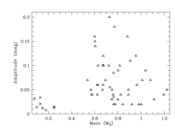
Figure 7: Photometric amplitude vs. mass for stars from the Open Cluster Database (triangles) and our targets (crosses). The detection limit for the solar-mass stars is 0.02 mag, explaining the lack of stars with very low amplitude in this sample.

From Fig. 7 it is obvious that solar mass stars show more frequently photometric variations with $A>0.05$ mag. According to a $\chi^{2}$ test, the amplitude distributions of both samples are significantly different ($\mathrm{FAP}<0.01$%). The lack of amplitudes larger than 5% on VLM objects can be explained with either a smaller relative spotted area, a more symmetric spot distribution, or lower contrast between spots and photospheric environment. The latter point seems to be more probable, since simulations show that the intensity contrast of the granulation pattern on M dwarfs is decreased by a factor of 14 in comparison with the Sun (Ludwig et al. lah02 (2002)). Symmetric spot distribution and low contrast, however, are predicted properties of a stellar surface governed by a turbulent dynamo, which might be the origin of magnetic activity on fully convective VLM objects (Durney et al ddr93 (1993)).

c) Compared with more massive stars, the fraction of objects with measurable photometric variation is significantly reduced among VLM objects. From our 26 targets, only 9 (35%) show significant periodic variability. In comparison, Krishnamurthi et al. (ktp98 (1998)) found periods for 21 out of 36 (i.e. 58%) stars in the Pleiades with masses from 1.2 to 0.5 $M_{\odot}$. Although these values might be biased by the incompleteness of the period search or the target selection (e.g., cluster members selected by X-ray activity), they support the notion for low spot coverage, low temperature contrast and/or symmetric distributions of spots on VLM objects, as outlined above.

5 The mass-period relation

To investigate the mass dependence of the rotation, we first compare our derived rotation periods with those of similar studies for more massive stars. From the Open Cluster Database, we collected a sample of rotation periods for solar mass stars in the Pleiades (see Sect. 1 for complete references). These stars have spectral types G, K, or early M, corresponding to masses from 1.2 to 0.5 $M_{\odot}$, and are thus complementary to our targets. We estimated masses for these comparison stars by comparing the V-band magnitudes with the 125 Myr isochrone of Baraffe et al. (bca98 (1998)), the same that we used to estimate masses for our VLM objects (Sect. 3.2). Therefore, we are confident that the absolute masses can be compared with each other, even if they are systematically offset because of an over- or underestimate of the assumed age of the Pleiades or shortcomings of the models.

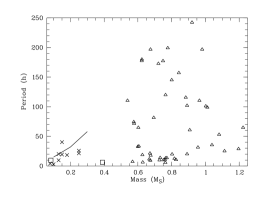
Figure 8: Rotation periods vs. mass: Our VLM rotation periods are shown as crosses. Triangles mark the periods for more massive stars from the Open Cluster Database (see Sect. 1 for complete references). The two squares show the periods from Terndrup et al. (tkp99 (1999)). The solid line marks a rough lower envelope to the observed $v\sin i$ values of Terndrup et al. (tsp00 (2000)).

In Fig. 8, we plot period vs. mass for our VLM objects (crosses), the solar-mass stars in the literature (triangles), and the two VLM stars from Terndrup et al. (tkp99 (1999), squares). Whereas solar mass stars show rotation periods up to 10 days, VLM objects have all periods below 2 days. However, we might have missed slowly rotating objects, e.g. because of spot evolution or absence of spots on these objects. For an independent evaluation of our upper period limit, we therefore compared our results with those of Terndrup et al. (tsp00 (2000) and references herein) who collected a large sample of spectroscopic rotational velocities for low-mass members of the Pleiades. We extracted a rough lower envelope of $v\sin i=$ 7, 10, and 15 kms^-1 for masses of 0.3, 0.2, 0.1$\,M_{\odot}$ from their Fig. 7. This lower $v\sin i$ envelope was transformed into an upper period envelope using the radii from the models of Chabrier & Baraffe (cb97 (1997)). These upper period limits are shown in Fig. 8 as solid line. With one exception, all our periods lie below this line, and are thus in good agreement with the $v\sin i$ data. Hence, all available data indicate a scarcity of slow rotators among VLM objects.

We used the $\chi^{2}$ test to compare our periods with those measured for solar-mass stars. The null hypothesis ’VLM objects and solar mass stars show the same period distribution’ is rejected with a FAP of $<0.01$%. Thus, the lack of slow rotators among VLM objects leads to a significant difference in the period distributions.

A second aspect of the mass-period relationship can be seen in Fig. 9, which is an enlargement of Fig. 8 for the VLM regime, containing period vs. mass for our nine VLM periods (crosses): Even in the VLM regime, the periods increase linearly with mass. A linear least-square fit to this period-mass relation gives $P=(105\pm 61)\,(M/M_{\odot})-(1.5\pm 10)$ h (dotted line in Fig. 9). This correlation, however, is not yet very strong: The correlation coefficient is 0.54, leaving a probability of 13% that periods and masses are uncorrelated. It is thus clearly necessary to substantiate the tendency of faster rotation with lower masses in the VLM regime by more measurements. In Fig. 9, we also show the two periods of Terndrup et al. (tkp99 (1999), squares). One of these periods is in good agreement with the linear fit, while the second one (for the object HHJ-409) is a clear outlier. The period, however, is convincing, and the probability that this star is not a cluster member is quite low (Hambly et al. hhj93 (1993)). Certainly, its period needs reconfirmation.

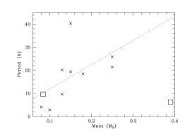
Figure 9: Period-mass relation in the VLM regime: Crosses are the nine periods determined in this work. The dashed line is a linear fit to their period-mass relation. The two squares indicate the two periods of Terndrup et al. (tkp99 (1999))

The positive correlation between period and mass is confirmed by observations in younger clusters. Herbst et al. (hbm01 (2001)) studied a large sample of periods for stars down to 0.1$\,M_{\odot}$ in the ONC (age 1 Myr). The median of their periods in the mass range $0.1<M<0.35\,M_{\odot}$ decreases steadily with mass. In SE2004, we demonstrate for the very young $\sigma$ Ori cluster (age 3 Myr) that this relationship extends to substellar objects. The period median from these two studies can be fitted as $P=(491\pm 26)\,(M/M_{\odot})-(7.9\pm 5.9)$ h, i.e. the slope is much steeper than for the Pleiades VLM stars. The flatter relationship for the Pleiades can be understood as a consequence of the pre-main sequence contraction process: In the course of their evolution from the age of $\sigma$ Ori to the age of the Pleiades, the radii of the VLM objects decrease, and therefore their rotation accelerates (see Sect. 6.1 for a detailed discussion of this process). The relative decrease of the rotation period is, however, only little dependent of mass. Hence, the period-mass relationship becomes flatter.

We note that for the ONC and the $\sigma$ Ori samples, the correlation is only apparent from the median of the periods, whereas in the case of the Pleiades the trend can be seen directly from the periods themselves. Since the positive correlation between rotation and mass is already present at very young ages, it must be produced in the earliest phases of rotational evolution, e.g. by mass-dependent angular momentum loss.

6 Rotational evolution of VLM stars

6.1 Modelling the rotational evolution of VLM stars

The periods for VLM objects in the Pleiades (from this work) and in the $\sigma$ Ori cluster (from SE2004) will now be combined to deliver constraints for models of angular momentum evolution in the VLM regime. Our goal is to see if a simple model can reproduce the period distribution in the Pleiades by transforming the $\sigma$ Ori periods to the Pleiades age. This transformation should take into account the basic ingredients of angular momentum evolution. We use the following nomenclature: The initial period of a given object in the $\sigma$ Ori cluster will be called $P_{i}$, and the corresponding evolved period for the Pleiades age $P_{e}$. Similarly, we will call the radii in the $\sigma$ Ori cluster and in the Pleiades $R_{i}$ and $R_{e}$. For the ages of the $\sigma$ Ori cluster and the Pleiades, we use $t_{i}$ and $t_{e}$. Note that our period search in the Pleiades is highly sensitive up to $P=300$ h, as shown in Sect. 3.3, whereas the study in $\sigma$ Ori is hampered by its less favourable time coverage, causing several windows of decreased sensitivity for $P>30$ h. Therefore, the transformation is done forward in time, to avoid unnecessary biases.

The rotational evolution of low-mass stars is, according to the current paradigm, determined by four factors:

a) The evolution starts with a given initial angular momentum. We use the period distribution in $\sigma$ Ori as starting point for the model.

b) Star-disk interactions probably play an important role for angular momentum regulation in the T Tauri phase. According to the so-called disk-locking paradigm (Camenzind c90 (1990), Königl k91 (1991)), young stars are locked to their disks and thus cannot spin up as long as the disk is not dissipated. However, because of inconsistent observational results, the disk-locking scenario remains controversial (see Stassun & Terndrup st03 (2003) for a detailed discussion). In SE2004, we showed that accretion disks are rare in the $\sigma$ Ori cluster. Therefore, for our purposes disk-locking to first order is neglectable, but we will keep in mind that it might play a role for some objects.

c) Rotation rates will be influenced by the contraction and the changes of the internal structure of the star. The latter point, however, can be neglected for fully convective objects, since their rotational behaviour should be insensitive to internal angular momentum transport (see Sills et al. spt00 (2000)). The contraction process can be modelled when the evolution of stellar radii is known. In case of angular momentum conservation, the rotation period will simply evolve with the square of the radius: $P_{e}=P_{i}(R_{e}^{2}/R_{i}^{2})$. We used the radii from the models of Chabrier & Baraffe (cb97 (1997)), although noting that these radii in the VLM regime are poorly verified by observations so far. The more recent models of Baraffe et al. (bcb03 (2003)), cover only the mass range up to $0.1\,M_{\odot}$, i.e. they end where the mass range of our objects begins, and are thus not suitable for our purposes. The radii from Baraffe et al. (bcb03 (2003)) are systematically smaller than in Chabrier & Baraffe (cb97 (1997)). For $M=0.1\,M_{\odot}$, the difference between both models is only 2% at the age of the Pleiades and around 10% at the age of $\sigma$ Ori. Thus, we could underestimate $P_{e}$ by a factor of $1.1^{2}/1.02^{2}=1.16$.

d) The final ingredient that determines rotational evolution is angular momentum loss through stellar winds. It has long been known that the rotational velocity of main sequence stars is proportional to stellar activity, and both decline with age following a $t^{-1/2}$ law (Skumanich s72 (1972)), i.e. the period is proportional to $t^{1/2}$. This simple model has been improved by Chaboyer et al. (cdp95 (1995)) to account for the ultrafast rotators in young open clusters. This modification introduces a saturation of the activity at high rotation rates, resulting in $P_{e}=P_{i}\exp{(t/\tau_{C})}$, where $\tau_{C}$ is the spin-down timescale (see Terndrup et al. tsp00 (2000), Barnes b03 (2003)). Increasing rotation rates for lower mass stars have been successfully modelled using a mass-dependent saturation level (Barnes & Sofia bs96 (1996), Krishnamurthi et al. kpb97 (1997)), which scales to the inverse of the global convective overturn timescale.

In the $\sigma$ Ori cluster, we measured rotation periods for 23 objects (SE2004). Ten of these periods were measured for stars with $0.075<M<0.3\,M_{\odot}$, the mass regime covered by our Pleiades targets. In the following, we use only these ten periods as $P_{i}$. For each of these objects, we determined the radius at 3 Myr (the most probable age for $\sigma$ Ori, see Zapatero Osorio et al. zbp02 (2002)) and 125 Myr (the age of the Pleiades). For most of these stars, there is only photometry available, disabling us from determining the radii empirically. Therefore, the radii were extracted from the models of Chabrier & Baraffe (cb97 (1997)), which are available for masses of 0.075, 0.08, 0.09, 0.1, 0.15, 0.2, 0.3$\,M_{\odot}$. For each object, we used the model for the mass nearest to the object mass. Thus, we obtained a list of $P_{i}$, $R_{i}$, and $R_{e}$, from which we now calculate $P_{e}$.

The rotational evolution can then be calculated as

$$P_{e}=\alpha P_{i}(R_{e}^{2}/R_{i}^{2})$$ (1)

In the following, we consider three different scenarios:

• $\alpha=1$: no rotational braking (model A)

• $\alpha=(t_{e}-t_{i})^{1/2}$: angular momentum loss through stellar winds following the Skumanich law (model B)

• $\alpha=\exp{(t/\tau_{C})}$: angular momentum loss through stellar winds with saturated activity (model C)

• $\alpha=\exp{(t/\tau_{C})}$: model C plus disk-locking (model D)

In Fig. 10, we show the rotational evolution for these scenarios. Model A is shown with dotted, model B with dash-dotted, model C with dashed and model D with solid lines. In the following, we discuss the results for each of the four models in detail.

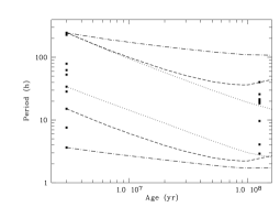
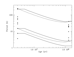
Figure 10: Rotational evolution of VLM objects: The upper panel shows the evolution of the rotation period for model A (no braking, dotted lined), model B (Skumanich braking, dash-dotted lines), and model C (exponential braking, dashed lines). In the lower panel, we compare model C (dashed lines) with model D (exponential braking with disk-locking, solid lines).

A) In this model, we simply assume no angular momentum loss, i.e. only hydrostatic contraction. In this case, the period evolution is fixed by $P_{i}$ and the evolution of the radii. For the periods at the Pleiades age, we obtain $P_{e}=0.28\ldots 17$ h. In Fig. 10 (upper panel), we show the period evolution for two objects (dotted lines). As can be seen from this Figure, half of the $\sigma$ Ori objects would end up with periods below the lower limit of the observed Pleiades periods. Thus, this approach is in clear contradiction to the observations in the Pleiades, since it produces too high rotation rates for all objects and does neither reproduce the upper nor the lower period limit. The lower limit of the known rotation periods of VLM objects lies at about 2 to 3 hours for ages of 3 Myr (Zapatero Osorio et al. zcb03 (2003)), 36 Myr (Eislöffel & Scholz es02 (2002)), 125 Myr (this work), and $\approx 1$ Gyr (Clarke et al. ctc02 (2002)), i.e. it seems to be nearly constant and independent of age. Since the objects surely undergo a significant contraction process, it becomes obvious that there must be significant rotational braking.

B) In the second model, we assume a Skumanich law for the rotational braking. Thus, the period evolution is determined only by the radii of the objects and the ages of the $\sigma$ Ori cluster $t_{i}$ and the Pleiades $t_{e}$. Using $t_{i}=3$ Myr and $t_{e}=125$ Myr (Zapatero Osorio et al. zbp02 (2002), Stauffer et al. ssk98 (1998)), we obtain periods of $1.7\ldots 110$ h at the age of the Pleiades. Three periods lie outside the limits defined by the observations in the Pleiades. In Fig. 10 (upper panel), we show the evolution for the slowest and the fastest rotator (dash-dotted lines). Remarkably, two objects end with periods larger than 100 h, in clear contradiction to the observations. Age uncertainties cannot explain this result, since we would have to choose $>10$ Myr for the age of $\sigma$ Ori and $<70$ Myr for the age of the Pleiades to bring both periods below 50 h. According to recent age determinations (Zapatero Osorio et al. zbp02 (2002), Stauffer et al. ssk98 (1998)), this is implausible. Similarly, it is not possible to explain these long periods with a possible overestimate of the radii, since this would only result in a decrease of about 16% (see above). Therefore, we can rule out rotational braking following the Skumanich law, even for the slowest rotators. This implies that the saturation limit for VLM objects lies beyond our maximum observed period of 240 h in $\sigma$ Ori, corresponding to a rotational velocity $<$5 kms^-1. Hence, all our $\sigma$ Ori objects are in the saturated regime. This is in agreement with recent studies: From Fig. 5 of Delfosse et al. (dfp98 (1998)) and Fig. 10 of Terndrup et al. (tsp00 (2000)), we infer upper limits of 3 kms^-1 and 6 kms^-1 for the saturation threshold.

C) In model C, we assume that all stars are beyond the saturation limit. Thus, the period evolution is determined by the radii of the objects and the spin-down timescale $\tau_{C}$. We considered two limiting cases by choosing $\tau_{C}$ either to reproduce the lower or the upper period limit in the Pleiades. If the model reproduces the lower period limit in the Pleiades of $P=2.9$ h, we obtain $\tau_{C}=54$ Myr. The periods at the age of the Pleiades then range from 2.9 to 109 h, and there are four objects with very long periods, which are not consistent with the available rotational data for the Pleiades, as already discussed for model B. Thus, it is more plausible to fix $\tau_{C}$ by reproducing the upper period limit of the Pleiades. Then, we obtain $\tau_{C}=150$ Myr and periods between 0.62 h and 41 h. For this scenario, we show the period evolution for two objects in Fig. 10 (upper panel, dashed lines). Compared with models A and B, model C with $\tau=150$ Myr clearly delivers the best fit to the data. There are, however, still three outliers in the $\sigma$ Ori period sample with very short periods at the age of the Pleiades, which are not consistent with the observations. These fast rotators will be discussed in Sect. 6.2.

D) This model includes two mechanism for angular momentum loss: exponential braking through stellar winds as in model C and disk-locking. For three of the ten $\sigma$ Ori objects (no. 14, 33, and 80), we have strong evidence that they possess an accretion disk. This can be inferred from near-infrared colour excess, large amplitude photometric variation, and accretion indicators in the spectra (see SE2004). For these three objects, we assume disk-locking up to an age of 5 Myr. Thus, the rotation period is constant from 3 to 5 Myr. This disk-locking scenario was combined with exponential braking, where the spin-down timescale was determined again by matching the upper limit of the period distribution in the Pleiades. In this case, we derived 250 Myr. In Fig. 10 (lower panel), we show the period evolution for the three objects with disk-locking (solid lines), and compare them to model C (dashed lines). Remarkably, two of the three outliers in $\sigma$ Ori from model C show signs of ongoing accretion. By including disk-locking for these objects, however, the fit to the observed data improves only marginally, as can be seen from Fig. 10 (lower panel). The period evolution for model C and model D is nearly indistinguishable. Thus, from our periods alone, there is no clear evidence for disk-locking on VLM objects.

Recapitulating, we state that a model with exponential angular momentum loss is able to reproduce our observed period distribution. We note that we cannot set definite constraints for the spin-down timescale from our data, since $\tau_{C}$ is extremely sensitive to changes in $R_{i}$ and thus the age of $\sigma$ Ori. Assuming an age of 8 Myr (the upper limit given by Zapatero Osorio et al. zbp02 (2002)), the values for $R_{i}$ decrease by a factor of 1.5, leading to a increased spin-down timescale of 300 Myr (with model C) and 950 Myr (with model D). Finally, we note that the definition of the lower and upper period envelope for the Pleiades is still limited by the small number of data points. Therefore, for a precise determination of $\tau_{C}$, better age estimates and more periods are needed. The influence of disk-locking could be excluded by using an older period sample as starting point.

With all these limitations in mind, we conclude that the spin-down timescale of VLM objects is most likely a few hundred Myr, and thus clearly longer than for solar-mass G-type stars (see Barnes b03 (2003)). Previous estimates of the spin-down timescale in the VLM regime are $\tau_{C}=246\pm 55$ Myr (Terndrup et al. tsp00 (2000)) and $\tau_{C}>1$ Gyr (e.g., Delfosse et al. dfp98 (1998), Barnes b03 (2003), Sills et al. spt00 (2000)). As noted above, more observational data are needed to enable a reliable assessment of $\tau_{C}$.

Recently, Barnes (b03 (2003)) proposed an appealing interpretation of stellar rotation periods, where the available period data is interpreted only in terms of the magnetic field configuration. According to this model, the available periods lie primarly on two sequences, called $I$ and $C$ sequence. The $I$ sequence produces slowly rotating stars, which exhibit large-scale, solar-type dynamos. On the other hand, stars on the $C$ sequence are exclusively fast rotators, because they only possess small-scale, convective magnetic fields. Due to their low masses, all our targets are fully convective (Chabrier & Baraffe cb97 (1997)). Therefore, all periods should belong to the $C$ sequence, for which an exponential spin-down and a lack of slow rotators is predicted. Although the model of Barnes (b03 (2003)) probably overestimates the spin-down timescales for VLM objects (see above), these predictions are in nice agreement with our results.

6.2 The fate of very fast rotators

Our periods in the Pleiades can be reproduced from the $\sigma$ Ori periods with a model including exponential braking (model C in Sect. 6.1). This model, however, still produces three $\sigma$ Ori objects with evolved periods $P_{e}$ below the lower limit of the period distribution in the Pleiades. Two of these fast rotators have $P_{e}<2\,h$. Although these outliers could be discussed away with the field star contamination of the $\sigma$ Ori targets and low number statistics, such an interpretation is not satisfying.

For our $\sigma$ Ori targets, the critical period $P_{crit}$, at which gravitational and centrifugal forces at the stellar surface are balanced (see Porter p96 (1996)), lies at $P_{crit}=3\ldots 7$ h, where the exact value depends on the mass of the object and the exact age of $\sigma$ Ori. Thus, two of the $\sigma$ Ori objects rotate nearly at breakup velocity.

The period evolution for these fast rotators (model C in Sect. 6.1) was compared with the evolution of the breakup period, which is determined by the evolution of the radii. As the stars contract, their periods decrease with $R^{2}$. On the other hand, $P_{crit}$ decreases only with $R^{1.5}$ (Herbst et al. hbm01 (2001)). Thus, we find that the fast rotators will probably approach the breakup velocity as they get older.

It is not clear what would happen if the rotation period of a star arrives at its critical period. One extreme scenario would be the complete disruption of the object after reaching its breakup velocity. In this case, our fast rotators in the $\sigma$ Ori sample would not reach the age of the Pleiades, and as a consequence the IMF should change somewhat with time. It seems, however, more probable that the disruption is avoided by throwing off surface material when approaching the critical velocity. Thus, the object might continue to evolve at or near the criticial period. In this scenario, the rotational evolution would be influenced by the mass loss, in the sense that an additional braking mechanism is involved. Moreover, the oblateness of the object, caused by its fast rotation, will increase its equatorial radius compared to a slowly rotating object. The models of Chabrier & Baraffe (cb97 (1997)), used for the model calculations of Sect. 6.1, neglect the influence of rotation on the evolution of the radii. For all these reasons, we conclude that the models of Sect. 6.1 are inappropriate for the fastest rotating $\sigma$ Ori targets.

We note that the oblateness of the fast rotators could induce periodic variability, if the object undergoes significant precession. In this case, the size of the visible surface is modulated by the rotation period. Therefore, it might be that the periodic variability of very fast rotators in the $\sigma$ Ori cluster is not caused by co-rotating spots on the surface, but by the oblateness and precession of the object.

7 Conclusions

We report a photometric monitoring campaign for VLM stars in the Pleiades. From lightcurve analysis, we derived rotation periods for nine Pleiades members with masses between 0.08 and 0.25$\,M_{\odot}$. Their periodic variability is likely caused by magnetically induced spots rather than inhomogenuously distributed dust clouds, since the targets are still too hot for dust condensation, but probably hot enough for magnetic surface activity. The lightcurves show very low amplitudes compared with more massive Pleiades stars, indicating that either the relative spotted area, the asymmetry of the spot distribution or the intensity contrast between spots and photosphere is reduced in the VLM regime. From our lightcurves, we see clear evidence for the temporal evolution of the spot patterns on timescales of about two weeks.

The rotation periods range from 2.9 h to 40 h, although our time series analysis is sensitive to periods up to 300 h. Comparing with the known periods for solar-mass stars in the Pleiades, we find a clear lack of slow rotators among VLM stars, in agreement with previous $v\sin i$ studies. In the VLM regime, the periods tend to decrease towards lower masses. Since this correlation has already been found for very young VLM objects, it must have its origin in the earliest phases of their evolution.

By combining the previously published periods for the young $\sigma$ Ori cluster (age 3 Myr, SE2004) with the periods in the Pleiades, we studied the rotational evolution in the VLM regime. Since the lower period limit is nearly constant at all ages, despite of the hydrostatic contraction process of the objects, there must be significant angular momentum loss. It was found that a Skumanich type angular momentum loss law ($P\propto t^{1/2}$) is not applicable in the VLM regime. Instead, the period evolution can be understood with saturated angular momentum loss following $P\propto\exp{(t)}$. We see no significant evidence for a contribution of rotational braking through star-disk interaction. Our best-fitting model cannot account for the fastest rotators in the $\sigma$ Ori sample. These objects rotate nearly at breakup velocity, and they will probably approach their breakup velocity as they get older. Therefore, their rotational evolution could be influenced strongly by mass loss and oblateness.

The observed lack of slow rotators and the exponential period evolution may be understood as a consequence of a convective magnetic field, as described by Barnes (b03 (2003)). All our targets are convective throughout their evolution, and thus unable to sustain a solar-type large-scale dynamo, which is the origin of the Skumanich type angular momentum loss law. Instead, VLM objects may exhibit small-scale fields, likely of turbulent nature, implying high rotation rates and an exponential spin-down, as observed. In addition, the turbulent dynamo scenario predicts rather symmetric spot distributions and weak surface activity, confirmed by the low lightcurve amplitudes.

Appendix A Period search in phase space

We investigated as alternatives the period search algorithms of Dworetsky (d83 (1983)) and Cincotta et al. (cmn95 (1995)) by applying them to the lightcurve of the object BPL129. For this object, our analysis (Sect. 3.2) reveals a convincing periodicity with $P=9.64$ h (see also Fig. 4). Any alternative period search method should also be able to recover this period.

In contrast to the frequency space based Fourier techniques, the methods of Dworetsky (d83 (1983)) and Cincotta et al. (cmn95 (1995)) work in phase space. They arrange the data points according to their phase for a number of test periods. For each period, they compute a statistical parameter, which allows to examine whether the time series contains this period. In the method of Dworetsky (d83 (1983)), this parameter is the ’string length’, the sum of the distances of the consecutive data points in phase space. If the time series contains a periodicity, the string length should show a minimum at this period. The algorithm of Cincotta et al. (cmn95 (1995)) relies on the entropy minimization of the lightcurve in phase space. Test parameter is the entropy, which should be normally distributed if no period is present (Cincotta et al. chm99 (1999)).

We computed string length and entropy for the lightcurve of BPL129. In Fig. 11, we show the results. Both plots show a local minimum at 9.6 h, the adopted period from our time series analysis. In both plots, however, there are many other lower minima. The string length distribution is very noisy, there exist many minima with similar depth. The global minimum lies at $P=82.1$ h, but the corresponding phase plot shows no periodicity at all. The reason for the failure of the algorithm is probably the large number of data points. Dworetsky (d83 (1983)) argues that his method is optimum for very few data points and random sampling. In the literature, the string length method is applied to lightcurves with typically less than 20 data points (e.g., Bouvier et al. bcf93 (1993), Joergens et al. jgn01 (2001)). Our results suggest that for many data points it is much more reliable to use Fourier techniques.

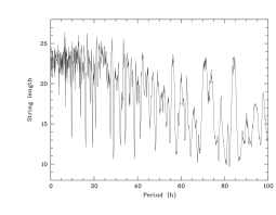
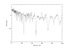
Figure 11: String length (upper panel) and entropy (lower panel) vs. period for the lightcurve of BPL129 (see text for explanation).

On the other hand, the entropy shows deep minima at multiples of one day, but the corresponding phase plots show no periodicity. From Fig. 2, it is obvious that for a period of one day all data points will have phases between 0.0 and 0.2 or between 0.8 and 1.0, leading to a minimized entropy. Hence, these minima are artifacts caused by the regular gaps between the observing nights. The method is therefore probably not useful for datasets with regular gaps.

Recapitulating, we found that both phase spaced techniques are not applicable to our data. For lightcurves with many data points and clumped data point distribution, Fourier techniques in combination with plausibility checks, as outlined in Sect. 3.2, are clearly superior and probably the best way to search for periods.

References

- (1) Adams, J. D., Stauffer, J. R., Monet, D. G., Skrutskie, M. F., Beichman, Ch. A., 2001, AJ, 121, 2053
- (2) Alard, C., Lupton, R. H., 1998, ApJ, 503, 325
- (3) Allard, F., Hauschildt, P. H., Alexander, D. R., Tamanai, A., Schweitzer, A., 2001, ApJ, 556, 357
- (4) Bailer-Jones, C. A. L., Mundt, R., 1999, A&A, 348, 800
- (5) Bailer-Jones, C. A. L., Mundt, R., 2001, A&A, 367, 218
- (6) Baraffe, I., Chabrier, G., Allard, F., Hauschildt, P. H., 1998, A&A, 337, 403
- (7) Baraffe, I., Chabrier, G., Barman, T. S., Allard, F., Hauschildt, P. H., 2003, A&A, 402, 701
- (8) Barnes, S. A., Sofia, S., 1996, ApJ, 462, 746
- (9) Barnes, S. A., 2003, ApJ, 586, 464
- (10) Bertin, E., Arnouts, S., 1996, A&AS, 117, 393, see also http://terapix.iap.fr/soft/sextractor
- (11) Bodenheimer, P., 1995, ARA&A, 33, 199
- (12) Bouvier, J., Cabrit, S., Fernández, M., Martín, E. L., Matthews, J. M., 1993, A&A, 272, 176
- (13) Bouvier, J., Stauffer, J. R., Martín, E. L., Barrado y Navascués, D., Wallace, B., Béjar, V. J. S., 1998, A&A, 336, 490
- (14) Bouvier, J., Forestini, M., Allain, S., 1997, A&A, 326, 1023
- (15) Camenzind, M., 1990, RvMA, 3, 234
- (16) Chaboyer, B., Demarque, P., Pinsonneault, M. H., 1995, ApJ, 441, 876
- (17) Chabrier, G., Baraffe, I., 1997, A&A, 327, 1039
- (18) Cincotta, P. M., Mendez, M., Nunez, J. A., 1995, ApJ, 449, 231
- (19) Cincotta, P. M., Helmi, A., Mendez, M., Nunez, J. A., Vucetich, H., 1999, MNRAS, 302, 582
- (20) Clarke, F. J., Tinney, C. G., Covey, K. R., 2002, MNRAS, 332, 361
- (21) Clarke, F. J., Oppenheimer, B. R., Tinney, C. G., 2002, MNRAS, 335, 1158
- (22) Dawson, P. C., De Robertis, M. M., 2000, AJ, 120, 1532
- (23) Delfosse, X., Forveille, T., Perrier, C., Mayor, M., 1998, A&A, 331, 581
- (24) Delfosse, X., Forveille, T., Segransan, D., Beuzit, J.-L., Udry, S., Perrier, C., Mayor, M., 2000, A&A, 364, 217
- (25) Durney, B. S., De Young, D. S., Roxburgh, I. W., 1993, SoPh, 145, 207
- (26) Dworetsky, M. M., MNRAS, 203, 917
- (27) Eislöffel, J., Scholz, A., 2002, ”The Origins of Stars and Planets: The VLT View”, Proc. of the ESO Workshop 2001, ed. McCaughrean & Alves, 219
- (28) Enoch, M. L., Brown, M. E., Burgasser, A. J., 2003, AJ, 126, 1006
- (29) Gelino, C. R., Marley, M. S., Holtzman, J. A., Ackerman, A. S., Lodders, K., 2002, ApJ, 577, 433
- (30) Gössl, C. A., Riffeser, A., 2002, A&A, 381, 1095
- (31) Hambly, N. C., Hawkins, M. R. S., Jameson, R. F., 1993, A&AS, 100, 607
- (32) Herbst, W., Bailer-Jones, C. A. L., Mundt, R., ApJ, 554, 197
- (33) Horne, J. H., Baliunas, S. L., 1986, ApJ, 302, 757
- (34) Joergens, V., Guenther, E., Neuh user, R., Fernández, M., Vijapurkar, J., 2001, A&A, 373, 966
- (35) Königl, A., 1991, ApJ, 370, 39
- (36) Krishnamurthi, A., Pinsonneault, M. H., Barnes, S., Sofia, S., 1997, ApJ, 480, 303
- (37) Krishnamurthi, A., Terndrup, D. M., Pinsonneault, M. H., Sellgren, K., Stauffer, J. R., et al., 1998, ApJ, 493, 914
- (38) Kürster, M., Schmitt, J. H. M. M., Cutispoto, G., Dennerl, K., 1997, A&A, 320, 831
- (39) van Leeuwen, F., Alphenaar, P., Meys, J. J. M., 1987,A&AS, 67, 483
- (40) Ludwig, H.-G., Allard, F., Hauschildt, P. H., 2002, A&A, 395, 99
- (41) Magnitskii, A. K., SvAL, 13, 451
- (42) Martín, E. L., Zapatero Osorio, M. R., Lehto, H. J., 2001, ApJ, 557, 822
- (43) Mathieu, R. D., 2003, IAUS, 215
- (44) Mohanty, S., Basri, G., 2003, ApJ, 583, 451
- (45) Moraux, E., Bouvier, J., Stauffer, J. R., Cuillandre, J.-C., 2003, A&A, 400, 891
- (46) Patten, B. M., Simon, Th., 1996, ApJS, 106, 489
- (47) Pinfield, D. J., Hodgkin, S. T., Jameson, R. F., Cossburn, M. R., Hambly, N. C., Devereux, N., 2000, MNRAS, 313, 347
- (48) Pinfield, D. J., Dobbie, P. D., Jameson, R. F., Steele, I. A., Jones, H. R. A., Katsiyannis, A. C., 2003, MNRAS, 342, 1241
- (49) Porter, J. M., 1996, MNRAS, 280, 31
- (50) Prosser, C. F., Schild, R. E., Stauffer, J. R., Jones, B. F., 1993, PASP, 105, 269
- (51) Prosser, C.F., Shetrone, M. D., Marilli, E., Catalano, S., Williams, S. D., Backman, D. E., Laaksonen, B. D., Adige, V., Marschall, L. A., Stauffer, J. R., 1993, PASP, 105, 1407
- (52) Prosser, C.F., Shetrone, M. D., Dasgupta, A., Backman, D. E., Laaksonen, B. D., Baker, S. W., Marschall, L. A., Whitney, B. A., Kuijken, K., Stauffer, J. R., 1995, PASP, 107, 211
- (53) Rebolo, R., Zapatero Osorio, M. R., Martín, E. L., 1995, Nature, 377, 129
- (54) Rebolo, R., Martín, E. L., Basri, G., Marcy, G. W., Zapatero Osorio, M. R., 1996, ApJ, 469, 53
- (55) Riffeser, A., Fliri, J., Gössl, C. A., Bender, R., Hopp, U., Bärnbantner, O., Ries, C., Barwig, H., Seitz, S., Mitsch, W., 2001, A&A, 379, 362
- (56) Roberts D. H., Lehar, J., Dreher, J. W., 1987, AJ, 93, 968
- (57) Scargle, J. D., 1982, ApJ, 263, 835
- (58) Scholz, A., Eislöffel, J., 2004, A&A, in press (SE2004)
- (59) Sills, A., Pinsonneault, M. H., Terndrup, D. M., 2000, ApJ, 534, 335
- (60) Skumanich, A., 1972, ApJ, 171, 565
- (61) Stassun, K. G., Terndrup, D., 2003, PASP, 115, 505
- (62) Stauffer, J. R., Schild, R. A., Baliunas, S. L., Africano, J. L., 1987, PASP, 99, 471
- (63) Stauffer, J. R., Schultz, G., Kirkpatrick, J. D., 1998, ApJ, 499, 199
- (64) Terndrup D. M., Krishnamurthi A., Pinsonneault M. H., Stauffer J. R., 1999, AJ, 118, 1814
- (65) Terndrup, D. M., Stauffer, J. R., Pinsonneault, M. H., Sills, A., Yuan, Y., Jones, B. F.; Fischer, D., Krishnamurthi, A., 2000, AJ, 119, 1303
- (66) Tinney, C. G., Tolley, A. J., 1999, MNRAS, 304, 119
- (67) Zapatero Osorio, M. R., Béjar, V. J. S., Pavlenko, Y., Rebolo, R., Allende Prieto, C., Martín, E. L., García López, R. J., 2002, A&A, 384, 937
- (68) Zapatero Osorio, M. R., Caballero, J. A., Béjar, V. J. S., Rebolo, R., 2003, A&A, 408, 663