Substructure Analysis of Selected Low Richness 2dFGRS Clusters of Galaxies

Abstract

Complementary one-, two-, and three-dimensional tests for detecting the presence of substructure in clusters of galaxies are applied to recently obtained data from the 2dF Galaxy Redshift Survey. The sample of 25 clusters used in this study includes 16 clusters not previously investigated for substructure. Substructure is detected at or greater than the 99% CL level in at least one test for 21 of the 25 clusters studied here. From the results, it appears that low richness clusters commonly contain subclusters participating in mergers. About half of the clusters have two or more components within $0.5\,h^{-1}\,\mathrm{Mpc}$ of the cluster centroid, and at least three clusters (Abell 1139, Abell 1663, and Abell S333) exhibit velocity-position characteristics consistent with the presence of possible cluster rotation, shear, or infall dynamics. The geometry of certain features is consistent with influence by the host supercluster environments. In general, our results support the hypothesis that low richness clusters relax to structureless equilibrium states on very long dynamical time scales (if at all).

1 Introduction

It is well recognized that many clusters of galaxies exhibit substructure where the operational definition of substructure adopted here will be departures from otherwise smooth galaxy density and velocity equilibrium distributions. Representative previous studies of samples of several clusters are given by, e.g., West & Bothun (1990), Rhee, van Haarlem, & Katgert (1991), Bird (1994), Escalera et al. (1994), West, Jones & Forman (1995), Pinkney, Roettiger, Burns, and Bird (1996), Girardi et al. (1997), and Solanes, Salvador-Solé, & González-Casado (1999). The presence of subclusters affects estimates of quantities such as the dynamical mass and mass-to-light ratio, the mean gravitational potential, and the global ellipticity. Substructure may also occur in the intracluster gas distribution traced by X-ray emission, and cross-correlating galaxy-gas structure is an important part of characterizing cluster dynamics (see, e.g., Davis et al. 1995, Bird, Davis, & Beers 1995, or references contained in the review article by Rosati, Borgani, & Norman 2002). In addition to determining the dynamical state of a cluster at a single epoch, the interaction of subclusters within the cluster (including mergers) can significantly affect dynamical evolution. Identifying and quantifying substructure may also reveal clues as to the initial conditions of the density perturbations from which clusters form and evolve.

The purpose of the present study is to apply a comprehensive, yet reasonably small, set of tests for substructure to recently obtained data from the 2dF Galaxy Redshift Survey (2dFGRS)(Colless 1998, Colless et al. 2001, and Maddox et al. 1998). With the large number of redshifts provided by the Survey, it is possible to explicitly correlate the substructure detected in the projected two-dimensional surface distribution with that found from three-dimensional tests combining positional and velocity information. This is usually sufficient to distinguish true substructure from projection effects including foreground and background contamination. Thus, the work presented in this paper is intended to provide survey results, identify potential trends and common characteristics, and highlight features warranting further study; it is not intended to necessarily provide a definitive last word.

Among its goals, the 2dFGRS is designed to allow investigation of the properties of galaxy groups and clusters by providing a large, homogeneous sample in redshift space. The source catalogue used as the Survey base is essentially a revised and extended version of the APM catalogue with target galaxies of extinction-corrected magnitudes $b_{J}\leq 19.45$ and redshifts with a measured RMS uncertainty of $85\>\mathrm{km}\,\mathrm{s^{-1}}$ (Colless et al., 2001). The median redshift of the catalogue is $z=0.11$. A preliminary study of the Survey database identified 431 Abell, 173 APM, and 343 EDCC clusters and provides precise redshifts, velocity dispersions, and updated centroids (De Propris et al., 2002). Additionally, this new data affords an opportunity to assess the completeness of, and contamination in, the older catalogues. The 25 clusters of galaxies listed in Table 1 to be studied here are selected from this new compilation, and include 16 clusters not previously investigated for substructure. The proper distances to each cluster at the epochs of emission and observation, $d_{p}(t_{e})$ and $d_{p}(t_{0})$, are calculated under the assumption of a flat universe with $\Omega_{\Lambda}=0.7$ and $\Omega_{m}=0.3$. All distances and linear scales are given in units of $h^{-1}$ Mpc where $h\equiv H_{0}/100$.

The last two columns of Table 1 contain the original richness classification (where available) as well as a revised richness based on the current 2dFGRS catalogue of clusters. Based on the memberships in the present catalogue, it can be seen that under the strict definition of the richness classes proposed by Abell (Abell, 1958), 9 of the 25 clusters in this study would be classified as “large groups” instead of low richness clusters. Nevertheless, these structures are included in this study under the (loose) heading of “low richness clusters”. Also note that since the membership completeness here is estimated at $80-90\%$, it is possible that 100% completeness would alter these richness estimates.

Table 1: The sample of 2dFGRS clusters selected for substructure analysis. Where available, and using the original definitions given by Abell, the original ACO richness classification R is given (Abell 1958 and Abell, Corwin, & Olowin 1989) along with the richness class determined from the 2dFGRS catalogue of clusters. The number in parentheses in the $\mathrm{R}_{2dF}$ column is the number of galaxies between $m_{3}$ and $m_{3}+2$ in the current catalogue. The proper distances $d_{p}(t_{e})$ and $d_{p}(t_{0})$ are given in $h^{-1}\,\mathrm{Mpc}$.

Cluster		N	RA(J2000)			Dec(J2000)			$d_{p}(t_{e})$	$d_{p}(t_{0})$	$\mathrm{R}_{ACO}$	$\mathrm{R}_{2dF}$
Abell	930	91	10,	7 ,	1.32	$-5$,	37 ,	28.7	162	171	0	0 (46)
Abell	957	90	10,	13 ,	38.42	$-0$,	55 ,	32.6	128	134	1	0 (35)
Abell	1139	106	10,	58 ,	10.98	1,	36 ,	16.4	113	118	0	$<0$ (20)
Abell	1238	86	11,	22 ,	54.36	1,	6 ,	51.2	203	218	1	$<0$ (23)
Abell	1620	95	12,	50 ,	3.89	$-1$,	32 ,	26.7	231	250	0	0 (49)
Abell	1663	94	13,	2 ,	52.55	$-2$,	31 ,	4.0	225	243	0	1 (72)
Abell	1750	78	13,	31 ,	11.00	$-1$,	43 ,	42.0	232	251	0	1 (51)
Abell	2734	125	0,	11 ,	21.60	$-28$,	51 ,	16.6	172	183	1	1 (72)
Abell	2814	87	0,	42 ,	8.82	$-28$,	32 ,	8.8	284	315	1	2 (83)
Abell	3027	91	2,	30 ,	49.41	$-33$,	6 ,	11.7	211	228	0	1 (51)
Abell	3094	108	3,	11 ,	25.00	$-26$,	55 ,	52.2	188	201	2	$<0$ (23)
Abell	3880	120	22,	27 ,	54.49	$-30$,	34 ,	31.3	161	171	0	$<0$ (25)
Abell	4012	73	23,	31 ,	50.89	$-34$,	3 ,	16.6	152	160	0	0 (44)
Abell	4013	85	23,	30 ,	22.62	$-34$,	56 ,	48.3	154	162	1	0 (30)
Abell	4038	154	23,	47 ,	34.92	$-28$,	7 ,	29.3	87	89	2	0 (39)
Abell	S141	110	1,	13 ,	47.09	$-31$,	44 ,	53.0	57	58	0	0 (33)
Abell	S258	87	2,	25 ,	44.44	$-29$,	36 ,	57.5	168	178	0	0 (36)
Abell	S301	95	2,	49 ,	33.72	$-31$,	11 ,	23.2	65	66	0	$<0$ (21)
Abell	S333	74	3,	15 ,	9.95	$-29$,	14 ,	37.4	185	197	0	0 (47)
Abell	S1043	111	22,	36 ,	27.96	$-24$,	20 ,	30.8	105	109	0	$<0$ (22)
APM	268	97	2,	29 ,	55.78	$-33$,	10 ,	37.2	212	228		0 (31)
APM	917	77	23,	41 ,	35.49	$-29$,	14 ,	10.9	144	151		$<0$ (22)
APM	933	124	23,	56 ,	27.66	$-34$,	35 ,	35.0	140	147		$<0$ (28)
EDCC	365	80	23,	55 ,	8.44	$-32$,	44 ,	26.0	165	175		$<0$ (28)
EDCC	442	127	0,	25 ,	31.36	$-33$,	2 ,	47.6	140	147		0 (36)

Among the previous substructure investigations involving relatively large samples of clusters is the study by Solanes, Salvador-Solé, & González-Casado (1999). This work considered subclustering in 67 rich clusters contained in the ESO Nearby Abell Cluster Survey (ENACS) catalogue. Using the best data available at the time, the ENACS catalogue is a reasonably homogeneous dataset with a completeness of $\sim 60-80\%$ (fraction of cluster members with redshifts), less but similar to that of the 25 2dFGRS clusters selected for this study. The completeness for the sample here is estimated to be $\sim 80-90\%$ for each cluster, and the sample contains all clusters in the 2dFGRS catalogue with $N\geq 70$. Two important differences between the ENACS study and this work are (1) the different test suites used to test for substructure, and (2) the average number of cluster members in the ENACS study is significantly less than here: the average membership in the ENACS study was $N=45$ with 48 of the 67 clusters having $N<50$, whereas the average membership number for this study is $N=99$ with the minimum number being $N=73$. This is important due to the dependence of the reliability and sensitivity of the statistical tests as a function of $N$.

The paper is organized as follows. Section 2 presents the method by which the ellipticity parameters, core radius, and central density are estimated. The tests used to detect the presence of substructure are described in Section 3 with a detailed analysis of the individual clusters presented in Section 4. A summary of the results and a concluding discussion are given in Section 5. Finally, Appendix 1 contains visualization plots for each cluster.

Table 2: Cluster Ellipticity and Position Angles. Position angles are measured counterclockwise from north (positive y-axis).

	R $=\sqrt{AB}\;h^{-1}$ Mpc
	0.50			0.75			1.00			1.25
Cluster	$\epsilon$	PA		$\epsilon$	PA		$\epsilon$	PA		$\epsilon$	PA
Abell 930	0.29	75		0.41	4		0.43	16		0.45	9
Abell 957	0.68	74		0.47	70		0.49	61		0.35	42
Abell 1139	0.25	117		0.42	98		0.20	62		0.04	73
Abell 1238	0.34	95		0.29	19		0.22	14		0.05	5
Abell 1620	0.08	1		0.49	17		0.50	39		0.17	41
Abell 1663	0.69	68		0.39	80		0.33	59		0.14	36
Abell 1750	0.43	4		0.74	12		0.62	34		0.54	39
Abell 2734	0.55	114		0.23	104		0.22	109		0.07	95
Abell 2814	0.30	100		0.27	130		0.50	127		0.40	120
Abell 3027	0.65	166		0.59	179		0.53	21		0.25	33
Abell 3094	0.55	5		0.49	160		0.37	141		0.33	138
Abell 3880	0.59	150		0.50	159		0.16	156		0.20	175
Abell 4012	0.42	14		0.37	1		0.36	118		0.01	133
Abell 4013	0.29	163		0.34	145		0.20	116		0.18	78
Abell 4038	0.43	21		0.36	18		0.21	156		0.50	96
Abell S141	0.67	0		0.66	168		0.63	169		0.58	168
Abell S258	0.75	114		0.69	113		0.71	104		0.58	104
Abell S301	0.36	161		0.45	32		0.61	48		0.54	48
Abell S333	0.59	152		0.49	156		0.47	131		0.41	132
Abell S1043	0.60	152		0.43	169		0.03	162		0.32	16
APM 268	0.71	172		0.52	4		0.35	3		0.20	177
APM 917	0.45	27		0.33	17		0.27	22		0.37	56
APM 933	0.53	145		0.40	128		0.03	160		0.30	17
EDCC 365	0.71	150		0.65	154		0.52	159		0.47	163
EDCC 442	0.34	33		0.54	20		0.58	38		0.45	35

2 Global Cluster Properties

Prior to applying tests for substructure, it is necessary to characterize each cluster in terms of global parameters such as a core radius and maximum central density, mean velocity and velocity dispersion, and global ellipticity and position angle. Here, “global” refers to the calculation of properties over an angular area that contains most or all cluster members. First, the cluster selection and foreground/background rejection methods are briefly summarized.

Essentially, this first catalogue of 2dFGRS clusters is a preliminary catalogue based on comparing the 2dFGRS results with previously identified clusters of galaxies sourced from the catalogues of Abell (Abell, 1958) and the revised/supplemented Abell (Abell, Corwin, & Olowin, 1989), APM (Dalton et al., 1997), and EDCC (Lumsden et al., 1992). The 2dFGRS catalogue was searched to identify clusters with centroids given in the above catalogues within $1^{\circ}$ of the centre of an observed survey tile. If the centroid of a catalogued cluster was found in a 2dFGRS tile, the 2dFGRS redshift catalogue was then searched for objects within a specified radius of the centroid. This process isolates a cone in redshift space containing candidate cluster members as well as foreground and background galaxies. The list of candidate members was then refined by inspection of the Palomar Observatory Sky Survey (POSS) plates. Finally, foreground and background contamination was eliminated (or significantly reduced) through subsequent detailed analysis of the redshift cone diagrams and, when necessary, redshift histograms. Further details concerning cluster selection can be found in De Propris et al. (2002).

2.1 Cluster Centroid and Ellipticity

Each galaxy position in $(RA,Dec)$ is converted to cartesian $(x,y)$ coordinates with relative separations calculated using the proper distance at photon time of emission, $d_{p}(t_{e})$. The cluster centroid is determined using an iterative search algorithm. A trial centre is computed from the arithmetic mean of all galaxies in the cluster, and is then recalculated using only the galaxies within an approximately 0.5 $h^{-1}$ Mpc radius of the initial centre. This process is repeated until it converges and the final centre determined. The reason for restricting the centroid computation in this manner is to avoid bias from large substructures well removed from the central regions.

For a quantitative measurement of cluster shape, it is convenient to use the dispersion ellipse of the bivariate normal frequency function of position vectors (see Trumpler & Weaver 1952) and first used to study cluster ellipticity by Carter & Metcalfe (1980). The dispersion ellipse is defined as the contour at which the density is 0.61 times the maximum density of a set of points distributed normally with respect to two correlated variables although the assumption of normally distributed coordinates is not necessary to achieve accurate shape parameters. Using the moments

$$\mu_{10}=\bar{x}$$ (1a)

$$\mu_{01}=\bar{y}$$ (1b)

$$\mu_{20}=\frac{1}{N}\sum_{i=1}^{N}x^{2}_{i}-\bar{x}^{2}$$ (1c)

$$\mu_{02}=\frac{1}{N}\sum_{i=1}^{N}y^{2}_{i}-\bar{y}^{2}$$ (1d)

$$\mu_{11}=\frac{1}{N}\sum_{i=1}^{N}x_{i}y_{i}-\bar{x}\bar{y}\;\;\mbox{,}$$ (1e)

the semi-principal axes of the ellipse $\Gamma_{A}$ and $\Gamma_{B}$ are the solutions of

$$\left|\begin{array}[]{cc}\mu_{20}-\Gamma^{2}&\mu_{11}\\ \mu_{11}&\mu_{02}-\Gamma^{2}\;\;\mbox{.}\\ \end{array}\right|=0$$ (2)

The position angle of the major axis with respect to north is then

$$\theta=\cot^{-1}\left(-\frac{\mu_{02}-\Gamma_{A}^{2}}{\mu_{11}}\right)+\frac{\pi}{2}$$ (3)

with $\Gamma_{A}$ ($>\Gamma_{B}$) being the semi-major axis, and the ellipticity is

$$\epsilon=1-\frac{\Gamma_{B}}{\Gamma_{A}}\;\;\mbox{.}$$ (4)

To achieve the best results, an iterative approach is adopted here similar to that used in previous studies such as Carter & Metcalfe (1980) or Burgett (1982). An initial circle of a given radius $R$ is defined about a trial centre and a new centre and dispersion ellipse are then calculated using only the galaxies contained within the circle. The semi-major and semi-minor axes $A$ and $B$ of the new ellipse are constrained to satisfy $R=\sqrt{A\,B}$. The process is repeated until convergence is achieved (usually requiring less than four iterations). It is possible for the iterative solution to become trapped in a local extremum, but this can be avoided by tracking each iteration. In applying the algorithm to the 18 richest clusters in the Dressler 1980 catalogue, it was noted that the results are sensitive to the presence of substructure (Burgett, 1982). The ellipticities and position angles for the 25 clusters are shown in Table 2 for four different average distances from the cluster centroids; the dispersion ellipses for mean radii of 0.5 and 1.0 $\mathrm{h}^{-1}$ Mpc are superimposed on the plots of galaxy positions in Appendix A for each cluster analyzed in Section 4.

Since a model density distribution can be significantly affected by ellipticity, this must be accounted for when constructing Monte Carlo catalogues of random clusters for comparison against actual data. Also note that it is sometimes nontrivial to distinguish true ellipticity from subcluster bias, and, in fact, the algorithm used to compute ellipticity can be used to also probe for substructure.

Table 3: Cluster Core Radii and Central Densities. The errors quoted are for the particular fit.

		$A_{c}$	$B_{c}$	$R_{c}\equiv\sqrt{A_{c}B_{c}}$	$\sigma_{0}$
Cluster		($h^{-1}$ Mpc)	($h^{-1}$ Mpc)	($h^{-1}$ Mpc)	gal/($h^{-1}$ Mpc)2
Abell	930	0.62	0.35	$0.47\pm 0.01$	$61\pm 2$
Abell	957	0.25	0.10	$0.16\pm 0.01$	$318\pm 1$
Abell	1139	0.33	0.21	$0.26\pm 0.01$	$138\pm 4$
Abell	1238	0.50	0.35	$0.41\pm 0.02$	$68\pm 3$
Abell	1620	0.57	0.40	$0.47\pm 0.02$	$59\pm 3$
Abell	1663	0.65	0.32	$0.46\pm 0.03$	$57\pm 4$
Abell	1750	0.61	0.25	$0.39\pm 0.03$	$41\pm 4$
Abell	2734	0.40	0.24	$0.31\pm 0.01$	$121\pm 5$
Abell	2814	0.43	0.30	$0.36\pm 0.01$	$81\pm 4$
Abell	3027	0.49	0.17	$0.29\pm 0.01$	$90\pm 3$
Abell	3094	0.53	0.29	$0.39\pm 0.01$	$88\pm 2$
Abell	3880	0.34	0.18	$0.25\pm 0.01$	$161\pm 13$
Abell	4012	0.46	0.17	$0.28\pm 0.01$	$71\pm 3$
Abell	4013	0.19	0.14	$0.17\pm 0.01$	$224\pm 2$
Abell	4038	0.23	0.15	$0.19\pm 0.01$	$261\pm 15$
Abell	S141	0.44	0.15	$0.26\pm 0.02$	$158\pm 18$
Abell	S258	0.51	0.15	$0.28\pm 0.04$	$108\pm 1$
Abell	S301	0.34	0.17	$0.24\pm 0.01$	$133\pm 9$
Abell	S333	0.52	0.24	$0.35\pm 0.01$	$62\pm 2$
Abell	S1043	0.44	0.22	$0.31\pm 0.01$	$107\pm 3$
APM	268	0.44	0.20	$0.30\pm 0.01$	$81\pm 3$
APM	917	0.17	0.12	$0.14\pm 0.01$	$270\pm 1$
APM	933	0.49	0.27	$0.36\pm 0.01$	$91\pm 2$
EDCC	365	0.56	0.25	$0.37\pm 0.01$	$70\pm 2$
EDCC	442	0.47	0.24	$0.33\pm 0.01$	$113\pm 4$

2.2 Density Profiles and Core Fitting

The assumed models for the density and velocity distributions are those for a cluster in dynamical and thermal equilibrium, viz., the empirical King approximation to an isothermal sphere and a Gaussian velocity distribution. It should be remembered that while the projected number density distributions of many clusters are fit well by King profiles, the core radius and central density are fitting variables that are convenient, but arbitrary, parameters for characterising the compactness of cluster central regions. In particular, the core radius has no intrinsic dynamical significance. Thus, the results presented in Table 3 should be regarded as comparative geometrical measures across the sample without dynamical implications. Similar considerations apply to the usage of the term ‘core’ throughout this paper.

For a circularly symmetric cluster projection, the two-dimensional surface King profile (King, 1972) takes the form

$$\sigma(r)=\frac{\sigma_{0}}{\displaystyle 1+\left(\frac{r}{R_{c}}\right)^{2}}\;\;\mbox{,}$$ (5)

where $\sigma(r)$ is the galaxy density at a distance r from the centre of the cluster, $\sigma_{0}$ is the maximum galaxy density of the cluster, and $R_{c}$ is the core radius of cluster. By extension, the two-dimensional King profile for an elliptically symmetric surface density distribution is

$$\sigma(x,y)=\frac{\sigma_{0}}{\displaystyle 1+\left(\frac{x}{A}\right)^{2}+\left(\frac{y}{B}\right)^{2}}$$ (6)

where $A$ and $B$ are the semi-major and semi-minor axes, respectively, and where it is conventional to define an equivalent mean core radius, $R_{c}=\sqrt{A\,B}$.

As a starting point, values of $R_{c}$ and $\sigma_{0}$ for the circular profile of Eqn. (5) are calculated using a least squares method. First, the expected galaxy count $n(r)$ at a given distance from the centre is found by integrating Eqn. (5),

$$n(r)=\pi R^{2}_{c}\sigma_{0}\ln{\left[(R^{2}_{c}+r^{2})/R^{2}_{c}\right]}\;\;\mbox{,}$$ (7)

and inverting for the radius $r(n)$ of the circle containing $n$ galaxies,

$$r(n)=R_{c}\sqrt{\exp{\left(n/\pi R^{2}_{c}\sigma_{0}\right)}-1}\;\;\mbox{.}$$ (8)

Each galaxy then becomes a data point in the merit function

$$\chi^{2}(R_{c},\sigma_{0})=\sum^{N}_{i=1}\left(\frac{r_{i}-r(i)}{\sigma_{i}}\right)^{2}\;\;\mbox{,}$$ (9)

where $r_{i}$ is the actual distance of the $i$th galaxy from the centre of the cluster and $r(i)$ is given by Eqn. (8). The minimisation of the merit function requires the derivatives with respect to parameters $R_{c}$ and $\sigma_{0}$ to be set equal to zero,

$$\frac{\partial\chi^{2}}{\partial R_{c}}=2\sum^{N}_{i=1}\left(\frac{r_{i}-r(i)}{\sigma^{2}_{i}}\right)\left(\frac{\partial r}{\partial R_{c}}\right)=0\quad\mbox{,}$$ (10a)

and

$$\frac{\partial\chi^{2}}{\partial\sigma_{0}}=2\sum^{N}_{i=1}\left(\frac{r_{i}-r(i)}{\sigma^{2}_{i}}\right)\left(\frac{\partial r}{\partial\sigma_{0}}\right)=0\quad\mbox{,}$$ (10b)

where

$$\frac{\partial r}{\partial R_{c}}=\frac{(\pi\sigma_{0}R^{2}_{c}-n)\exp{(n/\pi R^{2}_{c}\sigma_{0})}-\pi R^{2}_{c}\sigma_{0}}{\pi\sigma_{0}R^{2}_{c}\sqrt{\exp{(n/\pi R^{2}_{c}\sigma_{0})}-1}}\quad\mbox{,}$$ (11a)

and

$$\frac{\partial r}{\partial\sigma_{0}}=\frac{-n\exp{(n/\pi R^{2}_{c}\sigma_{0})}-\pi R^{2}_{c}\sigma_{0}}{2\pi\sigma_{0}R^{2}_{c}\sqrt{\exp{(n/\pi R^{2}_{c}\sigma_{0})}-1}}\quad\mbox{.}$$ (11b)

The Levenberg-Marquardt algorithm is then used to find the best fit for $R_{c}$ and $\sigma_{0}$ (Press et al., 1992).

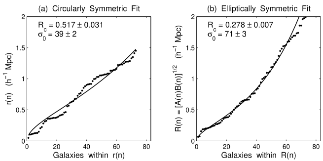
Figure 1: Comparison of the circular and elliptical King fits for Abell 4012. The solid line represents the expected count $n$ of galaxies for the fitted density model within either a circle of radius $r(n)$ (circular King profile) or a circle of geometric mean radius $R(n)\equiv[A(n)\,B(n)]^{1/2}$ for an ellipse with semimajor and semiminor axes $A(n)\mbox{,}\,B(n)$ (elliptical King profile). The points in each plot represent a galaxy at a specified distance from the cluster centroid. Points above the fit line are outside the test circle, but should have been inside at that distance; points underneath the fit line are within the test circle, but yield a higher density than the model density at that distance.

The circular fit above requires modification when the cluster core is highly elongated or multimodal. While it is straightforward to extend the fitting method above for the four free parameters in the elliptical King profile of Eqn. (6), it is possible to employ a simpler approach. If an ellipse with ellipticity $\epsilon$ is constructed such that $\sqrt{AB}=1h^{-1}$ Mpc $\equiv\sqrt{A_{R=1}B_{R=1}}\equiv R_{=1}$, then the coordinates of the perimeter satisfy

$$\frac{x^{2}}{A_{R=1}^{2}}+\frac{y^{2}}{B_{R=1}^{2}}=1\;\;\mbox{.}$$ (12)

Given the coordinates $(x_{i},y_{i})$ of the $i$th galaxy in the cluster, there exists a concentric ellipse which includes the coordinate $(x_{i},y_{i})$ defined by

$$\frac{x_{i}^{2}}{A_{i}^{2}}+\frac{y_{i}^{2}}{B_{i}^{2}}=1$$ (13)

This ellipse is defined by $\epsilon_{i}=\epsilon$ and $R_{i}=\sqrt{A_{i}B_{i}}$ with $R_{i}$ satisfying

$$R_{i}=R_{=1}\sqrt{\frac{x_{i}^{2}}{A_{R=1}^{2}}+\frac{y_{i}^{2}}{B_{R=1}^{2}}}\mbox{.}$$ (14)

The circular core fitting technique described above can now be utilized in the following manner:

1. Calculate values for the semi-major axis $A_{R=1}$ and the semi-minor axis $B_{R=1}$ using values for the ellipticity $\epsilon$ from Table 2 (this requires a certain amount of judgement to select the best values),

2. Transform the $(x_{i},y_{i})$ coordinates for each galaxy to $(x_{i}^{\prime},y_{i}^{\prime})$ for the coordinate system rotated to have the $x^{\prime}$-axis along the semi-major axis of the ellipse,

3. Calculate for all galaxies the quantity

   $$R_{i}=R_{=1}\sqrt{(x_{i}^{\prime})^{2}/A_{R=1}^{2}+(y_{i}^{\prime})^{2}/B_{R=1}^{2}}\quad\mbox{,}$$ (15)

4. Sort the values of $R_{i}$ in ascending order. This new order of galaxies, denoted by $n$, along with their values for $R_{i}(n)$, gives the number of galaxies found on or within the ellipse where $R$ = $R_{i}(n)$,

5. Use the above values for $R_{i}(n)$ in place of $r(n)$ used by the circular fitting algorithm to obtain new values for $R_{c}$ and $\sigma_{0}$ from the least-squares fit,

6. Recompute $A_{c}$ and $B_{c}$ using the original $\epsilon=1-B/A$ and $R_{c}=\sqrt{A_{c}\,B_{c}}$.

The results for elliptical surface density profile fits are shown in Table 3 for the 25 clusters. Comparisons of the results for the circular and elliptical fits shows that the fit to a circular profile provides a fair representation of the number distribution even when the actual shape is noticeably elongated. On average, compared to the elliptical profile, the circular fit also is better over the extent of the entire cluster. This can be due to the cluster ellipticity generally decreasing as a function of distance from the centroid as well as the circular fit essentially averaging over clumpy distributions that might bias the elliptical fit. However, the elliptical fit reproduces the density profile in the central regions significantly better than the circular fit for clusters such as, e.g., Abell 4012 (Figure 1).

For some clusters containing multi-component core regions such as Abell 930, the circular fit is slightly better than the elliptical fit in the central regions. This is presumably due to both components containing approximately the same number of galaxies so that the computed centroid is not at the centre of either component. Further detailed comparisons and fitting plots for all clusters can be found in  Vick (2004).

3 Tests for Cluster Substructure

The dangers of inferring the presence of substructure based on visual inspection of contour or gray scale plots alone is well known, yet this remains an appropriate component of a comprehensive test suite in order to better guide and interpret a statistical analysis. Two early studies utilizing contour plots to detect possible substructure in clusters of galaxies were conducted by Geller & Beers (1982) and Burgett (1982). In creating contour plots of clusters drawn from the Dressler (1980) catalogue, the Geller and Beers study applied a “boxcar smoothing” technique that was a best-available technique at that time. The improvements gained using an adaptive kernel approach to contour plotting are shown for many of these same clusters in Kriessler & Beers (1997). In addition to number density contours, the Burgett study presented luminosity-weighted contour plots of clusters in an attempt to correlate light with mass. As substructure studies have evolved with experience and numerical sophistication, it is now conventionally accepted that a synergistic combination of quantitative tests is necessary to detect different types of structure as well as to mitigate the results of false positives occasionally given by almost all estimators.

The test suite adopted for this study consists of a variety of one-, two-, and three-dimensional tests. These include visualization plots such as contour and nearest neighbor plots, velocity distribution statistics, and the $\alpha$ test (West & Bothun, 1990), $\beta$ test (West, Oemler, & Dekel, 1988), and $\kappa$ test (Colless & Dunn, 1996). For the latter three statistical tests, and for all clusters, a sample of 10,000 simulations was used to normalize the test and to determine the statistical significance. Use of the two point angular correlation function and the Fourier elongation test were considered but rejected on the grounds that they would not provide any new information compared to the chosen test suite.

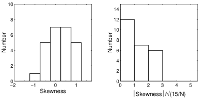
Figure 2: The skewness values for the 25 clusters with the standard deviation of the computed skewness value for a single cluster being approximately $\sqrt{15/N}$. From the figures it is evident that there is an excess of high skewness values over that expected if they were normally distributed.

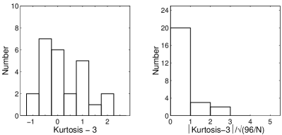
Figure 3: The kurtosis values for the 25 clusters with the standard deviation of the computed kurtosis value for a single cluster being approximately $\sqrt{96/N}$. From the figures it is evident that the velocity distributions for the majority cannot be distinguished from Gaussian distributions based solely on kurtosis values.

Table 4: Statistical moments of the cluster velocity distributions, equivalent standard deviations for the skewnness and kurtosis, and the confidence level (CL) derived from the $\chi^{2}_{vel}$ result for consistency with a Gaussian distribution. The entry for Abell S333* presents the velocity statistics for Abell S333 without the 8 galaxies in the group having $cz<18,500$ km/s, and the entry for Abell 4013* presents the velocity statistics without the 14 galaxies having $cz>17,500$ km/s.

Cluster		$\sigma_{vel}$	Skewness	# of	Kurtosis	# of	CL to reject
		(km/s)		$\sigma_{S}$		$\sigma_{K}$	Gaussian (%)
Abell	930	856	0.30	0.7	$-1.00$	1.0	$>$99.9
Abell	957	708	0.31	0.8	$-0.45$	0.4	49
Abell	1139	484	$-0.21$	0.6	0.18	0.2	76
Abell	1238	551	0.30	0.7	0.04	$<0.1$	14
Abell	1620	1001	0.77	1.9	0.65	0.6	97
Abell	1663	881	$-0.60$	1.5	0.86	0.8	36
Abell	1750	897	0.43	1.0	$-0.87$	0.8	98
Abell	2734	984	0.71	2.1	1.38	1.6	85
Abell	2814	894	$-0.14$	0.3	0.09	0.1	68
Abell	3027	838	$-0.57$	1.4	$-0.76$	0.7	99.9
Abell	3094	728	0.42	1.1	$-0.33$	0.4	93
Abell	3880	784	$-0.33$	0.9	$-0.02$	$<0.1$	36
Abell	4012	471	$-0.08$	0.2	0.37	0.3	96
Abell	4013	854	0.93	2.2	$-0.12$	0.1	$>$99.9
Abell	4013*	455	0.07	0.2	$0.15$	0.1	97
Abell	4038	835	$-0.04$	0.1	$-0.31$	0.4	96
Abell	S141	403	0.82	2.2	0.58	0.6	98
Abell	S258	557	0.07	0.2	$-0.52$	0.5	70
Abell	S301	679	$-0.01$	$<0.1$	1.92	1.9	99.9
Abell	S333	933	$-1.13$	2.5	1.04	0.9	99.9
Abell	S333*	573	0.01	$<0.1$	$-0.93$	0.8	93
Abell	S1043	1271	0.86	2.3	$-0.53$	0.6	$>$99.9
APM	268	769	$-0.65$	1.7	$-0.47$	0.5	98
APM	917	471	0.18	0.4	0.03	$<0.1$	73
APM	933	1033	0.77	2.2	0.81	0.9	97
EDCC	365	531	0.72	1.7	1.00	0.9	83
EDCC	442	726	0.00	$<0.1$	1.72	2.1	51

3.1 Velocity Statistics as a Substructure Indicator

The velocities for the galaxies in a relaxed cluster in thermal equilibrium are expected to be distributed normally with respect to any one cartesian coordinate. However, it should be recognized that taken by itself, an apparently non-Gaussian velocity distribution may reflect either a cluster not in equilibrium or a cluster containing one or more dynamically-bound subgroups embedded in an otherwise smooth, approximately equilibrium, distribution. Since all semi-invariants of higher order than two vanish identically for a Gaussian (normal) distribution, deviations from normality can be estimated by calculating the skewness and kurtosis (quantities proportional to the third and fourth order semi-invariants). In the following, all cluster redshifts have been transformed to velocities via the standard relativistic Doppler shift formula.

The skewness is given by

$$S=\frac{1}{\sigma^{3}}\left[\frac{1}{N}\sum^{N}_{i=1}(v_{i}-\overline{v})^{3}\right]$$ (16)

with $\overline{v}$ and $\sigma$ the mean velocity and standard deviation determined from the observed line-of-sight velocities $v_{i}$ of the $N$ cluster members. A positive (negative) value of $S$ implies the distribution is skewed toward values greater (less) than the mean. The kurtosis coefficient is defined as

$$K=\frac{1}{\sigma^{4}}\left[\frac{1}{N}\sum^{N}_{i=1}(v_{i}-\overline{v})^{4}\right]-3.$$ (17)

Because the kurtosis of a normal distribution is identically equal to 3, kurtosis values are conventionally presented with this subtracted from the result. Note that positive (negative) values of $K$ indicate distributions more strongly peaked (flatter) compared to normal distributions. Figures 2 and 3 show the distribution of the skewness and kurtosis values for the 25 clusters as well as estimates of their statistical significance in terms of the number of standard deviations away from the Gaussian values. Examples of previous studies of cluster structure using computed skewness and kurtosis to characterize the velocity distribution include Bird & Beers (1993), Ashman, Bird, & Zepf (1994), Bird (1994), West, Jones & Forman (1995), Pinkney et al. (1996), and Solanes, Salvador-Solé, & González-Casado (1999).

In practice, for a cluster containing $N\sim 50-100$ members, the skewness and kurtosis can provide suggestive but not necessarily definitive estimates as to whether a given distribution is significantly non-Gaussian. In order to obtain a better quantitative check for normality, it is convenient to use a $\chi^{2}$ statistic to estimate the probability that a test distribution can be distinguished from a Gaussian with the null hypothesis that the test distribution is, in fact, normal. To be reliable, the $\chi^{2}$ algorithm requires the binned test distribution to have a minimum number of datapoints in each bin to guarantee a reasonable probability for occupancy. This can be accomplished either by shifting/changing the number of fixed-width bins, or by using variable-width bins with (chosen) occupation probabilities above the minimum acceptable level. In testing the velocity distributions here, the adaptive method was implemented with a bin width varied to yield a minimum $5\%$ occupation probability for each bin.

Table 4 shows the velocity dispersion $\sigma_{vel}$, skewness $S$, the number of standard deviations $\sigma_{S}$ away from the skewness value expected for a normal distribution, kurtosis $K$, the number of standard deviations $\sigma_{K}$ away from the kurtosis value expected for a normal distribution, and the confidence level CL derived from the $\chi^{2}_{vel}$ test to reject the hypothesis of a normal distribution. Inspection of the results shows that 13 of the 25 clusters have catalogue distributions inconsistent with Gaussian distributions at $\geq 95\%$ confidence level (CL). Comparison of the $\chi_{vel}^{2}$ statistic with the skewness and kurtosis values shows no consistent correlation as to whether a distribution is (or is not) normal. In general, the skewness and kurtosis are not necessarily reliable indicators of departures from normality for these cluster membership sizes. However, it should be noted that even the $\chi^{2}$ test is not $100\%$ reliable, and the results depend somewhat on the degrees of freedom used in each case.

3.2 Contour, Segmentation, and Nearest Neighbor Visualization Plots

In spite of the dangers of giving too much weight to visual appearances, contour and other visualization plots remain useful when attempting to correlate the results of purely statistical tests to spatial structure or when comparing galaxy structure to gas structure revealed through X-ray emission. Thus, in the analysis of the clusters considered in this study, four different types of two-dimensional visualization plots are included in addition to the scatter plot of the galaxy positions.

The number density contour plots for the clusters are constructed with galaxy positions binned in $0.3\times 0.3\;(h^{-1}\,\mathrm{Mpc})^{2}$ square cells and then smoothing the contours with a bicubic interpolation algorithm. In order to provide a sufficient number of contour lines to give a visual sense of cluster structure, it was found that the sample could be broken into two general categories depending on whether, for a given cluster, any $0.3\times 0.3\;(h^{-1}\,\mathrm{Mpc})^{2}$ cell exceeded a count of 8 or more galaxies. For these clusters, contour levels were drawn at 20 gal/$(h^{-1}\,\mathrm{Mpc})^{2}$ intervals, while for clusters with no cell exceeding this threshold, contour lines were drawn at 10 gal/$(h^{-1}\,\mathrm{Mpc})^{2}$ intervals. In the first category (20 gal/$(h^{-1}\,\mathrm{Mpc})^{2}$) are Abell clusters 930, 957, 1139, 2734, 1663, 2734, 2814, 3094, 3880, 4012, 4013, 4038, S141, S258, S301, S1043, APM clusters 268, 917 and 933, and EDCC 442. In the second category (10 gal/$(h^{-1}\,\mathrm{Mpc})^{2}$) are Abell clusters 1238, 1620, 1750, 3027, and S333 and EDCC365.

As a means of comparing the cluster luminosity distribution to the number density distribution, we have also constructed luminosity-weighted contour plots. As for the number density contour plots, the initial cell size is $0.3\times 0.3\;(h^{-1}\,\mathrm{Mpc})^{2}$. The $k$-corrected absolute magnitude for each galaxy, $M_{J}$, is calculated using the standard Taylor expansion to first order in $z$ (see, e.g., Peebles 1993, pp. 328-330),

$$M_{J}=b_{J}-k-42.386+5\log_{10}h-5\log_{10}z$$

$$-1.086(1-q_{0})z+\,\ldots\;\;\mbox{,}$$ (18)

where $q_{0}=-0.55$ is the deceleration parameter value for $\Omega_{m}=0.3$ and $\Omega_{\Lambda}=0.7$. The $k$-corrections are computed from the emprical fits presented in De Propris et al. (2004). Each contour line represents an increase of $\approx 5\times 10^{10}\,L_{\bigodot}/(h^{-1}\,\mathrm{Mpc})^{2}$ (except for A2814 and A1750 which were set to $\approx 1\times 10^{11}\,L_{\bigodot}/(h^{-1}\,\mathrm{Mpc})^{2}$), and, as for the number density contours, the luminosity density contours are smoothed using bicubic interpolation.

The segmentation plots included in this study are meant primarily as a visual aid that provides a bridge between the density contour plots and the nearest neighbor plots described below. The basic idea is to connect “segments” of occupied cells to give some idea as to the location and extent of both connected and island regions in the cluster. Another appropriate terminology might be “tree”structure, but as that is used to denote a specific analysis technique, the term “segmentation” is used instead. The plot is constructed in much the same manner as are the contour plots: cell counts of galaxies are tabulated for a specified grid (again, $0.3\times 0.3\;(h^{-1}\,\mathrm{Mpc})^{2}$ square cells), the total number of cells is increased by subdividing the grid further in order to increase the resolution, and new cell counts are computed using the bicubic spline interpolation scheme as both an estimator and a smoothing mask. The segmentation algorithm is then simply the imposition of an additional step that thresholds the interpolated cell counts: the count is reset to zero for values below the threshold, and a user-defined gray scale is applied for counts above the threshold. In practice, we found the following choice of thresholds most useful:
1. For central core densities $\sigma_{0}<100\;\mathrm{gal}/(h^{-1}\;\mathrm{Mpc})^{2}$, the cutoff is 1.0 galaxy per bin (or, equivalently, $11.1\;\mathrm{gal}/(h^{-1}\;\mathrm{Mpc})^{2}$),
2. For central core densities $100<\sigma_{0}<200\;\mathrm{gal}/(h^{-1}\;\mathrm{Mpc})^{2}$, the cutoff is 1.5 galaxies per bin (or, equivalently, $16.7\;\mathrm{gal}/(h^{-1}\;\mathrm{Mpc})^{2}$),
3. For central core densities $\sigma_{0}>200\;\mathrm{gal}/(h^{-1}\;\mathrm{Mpc})^{2}$, the cutoff is 2.0 galaxies per bin (or, equivalently, $22.2\;\mathrm{gal}/(h^{-1}\;\mathrm{Mpc})^{2}$).
The resulting plot exhibits the connectivity of the cluster galaxy distribution as a function of cell count threshold.

A final visualization technique useful for identifying clumps that may represent true subclusters is the plot of nearest neighbors. The maximum distance used in order to define two galaxies as neighbors and the number of neighbors required to define a neighborhood of galaxies is, of course, arbitrary. In the plots presented in Appendix A, the selected distance is $0.25\,\mathrm{h}^{-1}$ Mpc and the minimum number of galaxies is set to four, i.e., each point on the plot is the position of a galaxy with four or more galaxies closer to it than $0.25\,\mathrm{h}^{-1}$ Mpc. Where appropriate, different choices are utilized to highlight certain features, and are presented in the detailed analyses of individual clusters.

3.3 The $\alpha$ Test

The 3-dimensional $\alpha$ test used to detect substructure in clusters of galaxies was introduced by West & Bothun (1990) and slightly revised by Pinkney et al. (1996). The test measures the shift in the arithmetic mean centroid of a cluster with the galaxy locations weighted by kinematics in specified neighborhoods about each galaxy. The centroid used is simply the arithmetic mean of all galaxy positions in the cluster. The location of each galaxy is weighted by the inverse of the velocity dispersion of nearby galaxies. Thus, a neighborhood of galaxies with similar velocities (i.e., low dispersion) has a higher weight and results in a centroid shift in their direction. If the member velocities are distributed randomly among the member positions, the centoid shift is statistically insignificant.

Thus, the steps leading to construction of the $\alpha$ statistic are as follows:

1. Convert (RA, Dec) sky coordinates to cartesian coordinates (x, y), and calculate the centroid of the two-dimensional galaxy distribution,

   $$x_{c}=\frac{1}{N}\sum_{i=1}^{N}x_{i},\mbox{ and\ }y_{c}=\frac{1}{N}\sum_{i=1}^{N}y_{i}.$$ (19)

2. Assign a weight $w_{i}=1/\sigma_{i}$ to each galaxy, where $\sigma_{i}$ is the line of sight velocity dispersion for galaxy $i$ and its $N_{nn}$ nearest neighbors where an arbitrary choice is made to set $N_{nn}=\sqrt{N}$,

3. For each galaxy $i$ and its $N_{nn}$ nearest neighbors, calculate the weighted centroid,

   $$x^{\prime}_{c}=\frac{\sum_{i=1}^{N_{nn}+1}x_{i}w_{i}}{\sum_{i=1}^{N_{nn}+1}w_{i}}\mbox{ and }y^{\prime}_{c}=\frac{\sum_{i=1}^{N_{nn}+1}y_{i}w_{i}}{\sum_{i=1}^{N_{nn}+1}w_{i}}.$$ (20)

4. The difference in centroid of these nearest neighbor velocity groups and the unweighted centroid is calculated,

   $$\alpha_{i}=\sqrt{\left(x_{c}-x^{\prime}_{c}\right)^{2}+\left(y_{c}-y^{\prime}_{c}\right)^{2}}$$ (21)

5. Finally, the $\alpha$ statistic quantifies the cluster substructure as an average of the $\alpha_{i}$ values,

   $$\alpha=\frac{1}{N}\sum_{i=1}^{N}\alpha_{i}.$$ (22)

The test is normalized by comparison with the value $\alpha$ takes for Monte Carlo distributions created by randomly shuffling the velocity among galaxy positions fixed by the data. The $\alpha$ statistic for the cluster is compared to the mean $\alpha$ statistic from Monte Carlo simulations with the difference expressed in standard deviations used to estimate the probability for the presence of substructure. A subcluster will influence the centroid of its velocity group provided it deviates from the global distribution both spatially and in velocity dispersion. Detailed results of the $\alpha$-statistic computed for the clusters themselves as well as for the Monte Carlo simulations are contained in Vick (2004).

3.4 The $\beta$ Test

The $\beta$ test is used to detect deviations from mirror symmetry about the cluster centre where mirror symmetry is defined as a 2-dimensional coordinate inversion $(x,y)\rightarrow(-x,-y)$ (West, Oemler, & Dekel, 1988). After determining the cluster centroid, the mean distance to each galaxy’s nearest neighbors is calculated. Then, the location of the inverted position of each galaxy is computed, and the mean distance from that location to the nearest neighbors is calculated. Actual mean distances are compared to the mirror image distances. Large differences indicate asymmetry and possible substructure. This test is particularly useful in quantifying visual impressions of asymmetry conveyed by the visualization plots, and can often be correlated with results from the ellipticity algorithm.

Here, the asymmetry parameter for galaxy $i$ is defined as

$$\beta_{i}=\log{\left(\frac{d_{0}}{d_{i}}\right)}$$ (23)

where $d_{0}$ is the mean distance of the galaxy’s $N_{nn}$ nearest neighbors ($N_{nn}=\sqrt{N}$ rounded to the nearest integer), $d_{i}$ is the mean distance of the mirror image point of each galaxy to the $N_{nn}$ nearest neighbors, and $N_{Total}$ is the number of total galaxies in the cluster. The $\beta$ statistic for a cluster is the mean $\beta$ value for all the galaxies times one thousand or

$$\beta=1000\left\langle\beta_{i}\right\rangle.$$ (24)

The significance of the $\beta$ statistic of the data is estimated by comparison against a distribution obtained from Monte Carlo simulation. This is accomplished by holding constant the distance from the centre of each galaxy in the data, but uniformly varying the polar angle from 0 to 2$\pi$. The galaxy coordinates are then relocated at $x_{i}=r_{i}\cos{\phi}$ and $y_{i}=r_{i}\sin{\phi}$. The $\beta$ statistic is recalculated for each reshuffled galaxy cluster. The mean and standard deviation computed from the Monte Carlo simulations are then compared to the value from the original data. A Monte Carlo probability of random occurrence is used to estimate the significance of any deviation from mirror symmetry. A significant deviation may indicate an asymmetrical distribution caused by one or more subclusters. Detailed results for both the $\beta$-statistic computed for the clusters as well as for the Monte Carlo simulations are contained in Vick (2004).

3.5 The $\kappa$ Test

The $\kappa$ test is a three-dimensional substructure test based on nearest neighbor velocity relationships first introduced in a substructure study of A1656 (Colless & Dunn, 1996). As discussed in that study, the $\kappa$ test is similar in intent to the Dressler-Shectman $\Delta$ test (Dressler & Shectman, 1988) in that it probes deviations in localized velocity variations compared to the global cluster velocity distribution. It is especially useful for detecting subgroup dynamics in a cluster core region including the case of a projected subgroup centroid overlapping the projected cluster centroid.

The velocity distribution of a user-selected number of nearest neighbors $n$ is compared to the velocity distribution of the entire cluster with the test statistic $\kappa_{n}$ constructed as

$$\kappa_{n}=\sum^{N}_{i=1}-\mathrm{log}[P_{KS}(D>D_{obs})]\;\;\mbox{,}$$ (25)

where the sum is over the $N$ galaxies in the cluster. Thus, $P_{KS}(D>D_{obs})$ is the probability that the K-S statistic $D$ is greater than the observed value $D_{obs}$ which is simply a standard K-S two sample test with a significance that can be computed in a straightforward manner as given in, e.g., Press et al. (1992). The $\kappa$ statistic is then the (negative) log-likelihood that there is no localized deviation in the velocity distribution on the scale of sets of $n$ nearest neighbors. The larger the value of $\kappa$, the greater the likelihood that the local velocity distribution is different from the overall cluster velocity distribution. The significance of $\kappa_{n}$ can also be computed from Monte Carlo simulations by randomly shuffling the velocities of the individual galaxies while holding their positions constant.

For this study, the default number of nearest neighbors is set to $\sqrt{N}$, but the results are relatively insensitive to the precise choice when it is $\sim\sqrt{N}$; see Vick (2004) for a detailed comparison between the $\kappa$ and $\Delta$ tests as well as the sensitivity of the $\kappa$ test to the selected number of nearest neighbors. It is convenient to display the results utilizing “bubble skyplots” where at each galaxy position, a circle is drawn of radius proportional to the log-likelihood of the local and overall distributions not being the same under the K-S two-sample test. In this paper, the radii of the $\kappa$ bubbles was set to $\kappa_{n}/30$ for visualization purposes.

4 Detailed Analysis of Individual Clusters

This section provides a detailed analysis of the individual clusters from consideration of the results of the statistical tests combined with visualization plots. It will be seen that while detecting substructure is straightforward, unambiguous interpretation remains problematic. Further correlation with X-ray data is expected to remove some ambiguities, especially as relates to cluster membership. The projected (2-dimensional) galaxy separations are inferred from the proper distance at photon time of emission, $d_{p}(t_{e})$.

4.1 Abell 930

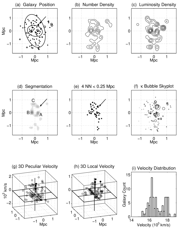
Figure 19: Visualization plots for Abell 930.

From Figures 19(a)-(e), inspection of Abell 930 surface plots shows a low density, moderately elliptical cluster containing a (projected) bimodal central region aligned east to west with the two components having a projected separation of approximately $0.50\,h^{-1}$ Mpc. Outside the core there is a relatively high density region (greater than 40 galaxies per ($h^{-1}$ Mpc)²) located approximately $1.0\;h^{-1}$ Mpc due north of the cluster centre. The segmentation and nearest neighbor plots, Figures 19(d)-(e), again highlight the two-component core region (labels A and B) and concentration of galaxies to the north (label C). As discussed below, these three components appear to be 3-dimensional structures as well.

In spite of the relatively high concentration of galaxies to the north, the $\beta$ test yields no indication of global asymmetry ($P_{\beta}$ = 30%). This is due to the positioning of the clustre center between the two components in the central regions; positioning the center at the centre of one of these components would result in a significant asymmetry signal. This re-positioning was not done for this cluster as for others in this sample because of the near equality in number density and total number of galaxies in each of the components, and the lack of an X-ray map that might indicate which of the components possesses more mass.

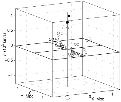
Figure 4: Local velocities of the nearest neighbors in Figure 19(e) for Abell 930.

The ellipticity computation yields an $\epsilon$ = 0.29 – 0.45 over the entire test range from radius R = 0.50 – 1.25 $h^{-1}$ Mpc (Table 2). As expected, the mean radius of $R=0.50\;h^{-1}$ Mpc results in a position angle aligned approximately east to west due to the bimodal core ($PA=75^{\circ}$). Average dispersion ellipse radii from $R$ = 0.75 - 1.25 $h^{-1}$ Mpc are aligned from north to south with an average position angle of $PA\approx 10^{\circ}$. We use an average ellipticity and position angle $\epsilon$ = 0.4, $PA=70^{\circ}$ to calculate a core radius and central density of $R_{c}=0.47\pm 0.01$ and $\sigma_{0}=61\pm 2$.

Inspection of the velocity distribution in Figure 19(i) shows a bimodal profile with the two peaks separated by approximately 1500 km/s. Comparison of the members of the two spatial core components to the two velocity modes yields no relationship, but due to this bimodality, the $\chi^{2}_{vel}$ velocity test rejects the hypothesis of normality with $>99.9\%$ CL (Table 4).

The 3D plots and tests also indicate the presence of substructure (Figures 19(f)-(h)and Table 6). In particular, the peculiar velocity plot of Figure 19(g) shows the two-component central region in the 2D plots separating into the main body of the cluster with peculiar velocities less than zero (due to the averaging of the two peaks to arrive at the cluster mean velocity) while approximately 15 galaxies have peculiar velocities of $<1000\,\mathrm{km/s}$ (this is the eastern component seen in the 2D plots). It is easier to distinguish the western (A), eastern (B), and northern (C) components in the central regions as distinct subgroupings by plotting the local velocities of only the nearest neighbors (see Figure 4). It should also be noted that the possibility cannot be excluded that each of these two larger groupings may contain finer-detailed structure not resolved here, or that there is additional structure to the north.

Both the $\alpha$ and $\kappa$ tests indicate some level of substructure with probabilities of random occurrence of 3.0% and 5.8%, respectively. The $\kappa$ bubble skyplot presented in Figure 19(f) shows two areas of possible subclustering: a group of seven galaxies show relatively large radii bubbles (indicating high $\kappa$ statistics) from $0.5-1.0\,h^{-1}$ Mpc north of the centre, and a second group of above average-sized bubbles includes galaxies in the western component of the core region. Among the seven galaxies to the north with relatively high $\kappa$ values, three of the seven are well separated from a compact grouping of four galaxies indicated by the arrows in Figures 19(a), (e), and (f) (two have nearly coincident angular positions and are indistinguishable in the 2D plots). Due to their apparent proximity coupled with the results of the $\kappa$ test, and the fact that these four galaxies possess velocities consistent with cluster membership, we hypothesize that they comprise a dynamically bound subgroup belonging to the cluster.

In summary, there appears to be significant substructure present in this cluster. The substructure of the central region makes Abell 930 a potential site for merger dynamics, the velocity structure is also potentially significant, and there are probably at least one or two bound subclusters well removed from the central regions.

4.2 Abell 957

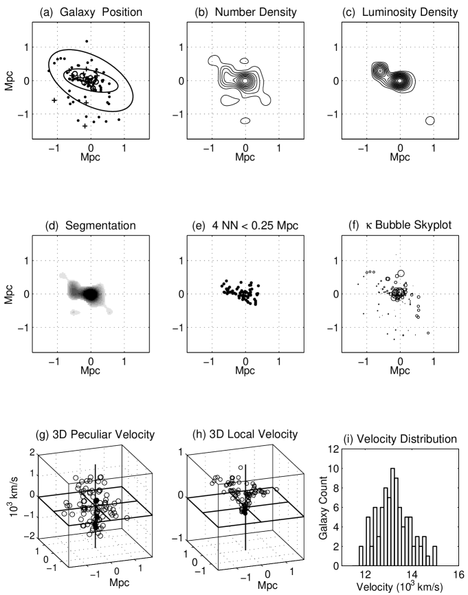
Figure 20: Visualization plots for Abell 957.

Abell 957 possesses a dense core with a core radius $R_{c}=0.16\pm 0.01\,h^{-1}$ Mpc and a central density $\sigma_{0}=318\pm 1$ (see Figures 20(a),(b),(d)). In both two and three dimensions, the cluster central regions are distinctly bimodal, with a second high density concentration of galaxies approximately 0.5 $h^{-1}$ Mpc east of the core also possessing a large fraction of the total luminosity due to two relatively bright galaxies whose velocities are consistent with cluster membership (see Figure 20(c)). Due to a selection effect in the catalogue, a very bright D galaxy residing at the centre of the peak number density that is a well-established cluster member (based on redshift as well as sky location) was not included in the present sample. However, we have added it to the sample, and have also re-positioned the cluster center to coincide with the location of peak number density. As can be seen by comparing Figures 20(b) and (c), the peak luminosity coincides with the peak galaxy density at the position of the D galaxy.

With a probability for random occurrence of $P_{\beta}=0.5\%$, the $\beta$ test detects the asymmetry due to the single structure east of the core. The bimodal characteristic gives the cluster a highly elongated shape (see Table 2 and Figure 20(a)) leading to $\epsilon=0.68-0.35$ from $R=0.50-1.25h^{-1}$ Mpc, and where the semimajor axis is consistently aligned with the two central components in this range with a $PA=74^{\circ}-42^{\circ}$. Even at larger distances from the centre, with the outer regions being relatively diffuse, the dispersion ellipses are strongly influenced by the dense central region. However, from Figure 20(d), it can be seen that the core itself possesses some ellipticity with a position angle pointed directly toward the eastern subgroup, possibly indicating tidal interactions between these two central components.

Considered in its entirety, the velocity distribution is consistent with a normal distribution. However, note from Figure 20(a) that the 0.5 $h^{-1}$ Mpc dispersion ellipse region contains several galaxies with velocities that are slower (open circles) and faster (plus signs) by more than $1.3\sigma$ compared to the cluster mean velocity. While the $\kappa$ test for the entire cluster shows no significant signal with $P_{\kappa}=14.4\%$, four galaxies in the core show a 5% or less probability that the average of their nearest neighbor velocities belong to the clusters velocity distribution (see Figures 20(g)–(h)). In particular, some of these galaxies may form part of a small subcluster with projected (surface) centroid nearly coincident with the core centroid (see Figure 20(h)), and it is the relatively slow local velocities giving rise to the large bubbles in Figure 20(f). This may be evidence for a line-of-sight merger.

Although the $\kappa$ test does not indicate anything significant in the eastern subgroup, it is not unreasonable to speculate that this group may still be moving toward or away from the core in a direction perpendicular to the line of sight. It should also be noted that Rosat All Sky Survey (RASS) data does exist for this cluster, and confirms that the cluster’s central potential well is very close to the computed centroid of the core. The region appears dynamically active, and also hints that the eastern clump is, in fact, a bound subgroup. However, the RASS observations provide only 454s of exposure time. This cluster is also at the edge (44’ off-axis) of a PSPC observation with a total of 1.95 ksec. A much longer exposure time with better resolution is required to infer further dynamical properties.

In previous studies of this cluster, the bimodal core has been identified by Beers et al. (1991) and Kriessler & Beers (1997). The analysis presented in Beers et al. (1991) concludes that the two components are not grabvitationally bound, but uncertainty in the radial velocity difference does allow for bound solutions. With the larger sample of redshifts available here, this question will be investigated further in a following paper. Using redshift data for 34 galaxies, Solanes, Salvador-Solé, & González-Casado (1999) found the velocity distribution to be consistent with a normal distribution with statistics similar to those presenterd here for 90 galaxies. The Solanes et al. study also performed the $\Delta$ test with a result of $P_{\Delta}=3.4\%$ compared to results found here of $P_{\Delta}=17\%$.

4.3 Abell 1139

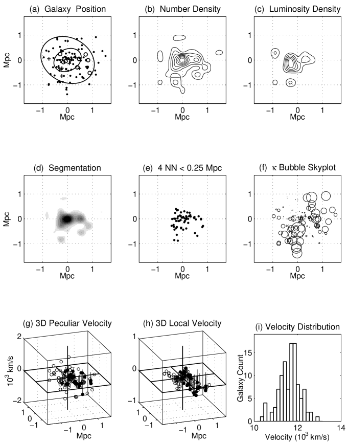
Figure 21: Visualization plots for Abell 1139.

The analysis of A1139 presented here is based on 106 galaxies. The fitted optical core radius of Abell 1139 is $0.26\,h^{-1}\,\mathrm{Mpc}$ with a central density of 138 which is fairly typical of the poor clusters in this sample. Figure 21(b) shows the core and the more asymmetric envelope. The azimuthally averaged fits to the cluster shape are not sensitive to the relatively low density concentration of galaxies seen to the west of the core at ($0.75$, $-0.2$) Mpc (see Figure 21(d)). At large radii the ellipticity is low, $\sim 0.2$, and the position angle is $\sim\,65^{\circ}$. The inner part of this cluster is elongated and the ellipticity within 0.75 Mpc is $\approx\,0.4$ with a position angle of $\approx\,100^{\circ}$ reflecting the core elongation seen in the number density map. It should be noted that there are three additional relatively bright galaxies located near the centre of this cluster having redshifts consistent with cluster membership that are not included in the 2dFGRS catalogue. Their inclusion shifts the centre of luminosity toward the number density centroid compared to the sample of 106 galaxies used here, but does not alter any of the results concerning substructure.

The two-dimensional $\beta$ test indicates no significant asymmetry ($P_{\beta}=15\%$). However, the three-dimensional $\alpha$ and $\kappa$ tests indicate the presence of strong substructure, each with a probability of $<0.1\%$ that the values are drawn from a relaxed distribution. The bubble plot in Figure 21(f) shows the two disjoint areas that deviate from the cluster mean lying to the west at (1.0, 0.0) Mpc and south (0.0, $-1.0$) Mpc of the main cluster component. These two systems can be seen in the number density plot (Figure 21(b)) as low-level extensions from the main cluster. These two structures are also seen in the nearest neighbor plots (Figure 21(e)). The segmentation plot (Figure 21(d)) shows the core and western subclump clearly while only a hint of the southern subclump is evident, but both substructures can been seen in the local velocity plot (Figure 21(h)).

Intriguingly, an inspection of the local velocity plot indicates that there is a velocity gradient across the cluster. This shear seen in the velocity structure may indicate that this cluster has a significant rotation. Alternatively, the cluster may be in the late stages of a double merger with two subclumps spiraling in to merge with the main system.

In contrast to the $\alpha$ and $\kappa$ tests, the velocity distribution in Figure 21(i) does not show any statistical evidence for substructure (See Table 4). In addition, the velocity dispersion of 484 km/s is somewhat on the low side for the poor clusters in this sample. However, the three-dimensional tests and the cluster morphology indicate that this cluster is dynamically interesting. This along with the possible presence of a velocity gradient in the system indicates that additional data from X-ray observations would be useful in clarifying the dynamical state.

Previous investigations of this cluster have found little or no evidence for substructure, and have not identified the velocity gradient found here. In particular, Kriessler & Beers (1997) and Krywult, MacGillivray, & Flin (1999) concluded that the cluster is unimodal with no substructure while West & Bothun (1990) found marginal evidence for substructure.

4.4 Abell 1238

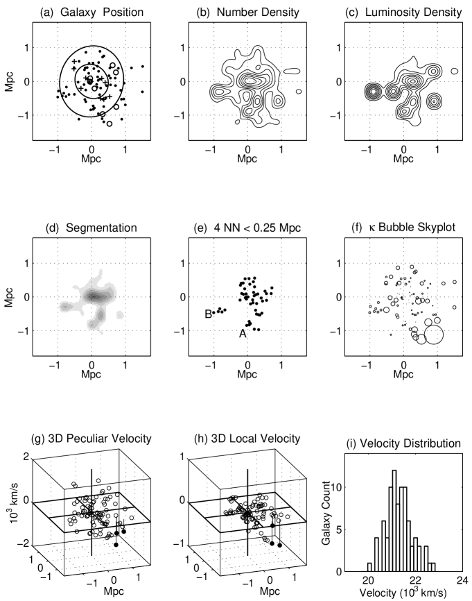
Figure 22: Visualization plots for Abell 1238.

With a central density of $\sigma_{0}=68\pm 3\,\mathrm{gal}/(h^{-1}\mathrm{Mpc})^{2}$, Abell 1238 is a relatively low density cluster with a somewhat irregularly shaped central region of core radius $R_{c}=0.41\pm 0.02\,h^{-1}\,\mathrm{Mpc}$ (see Figures 22(a), (b), and (d)). In general, the cluster has a low ellipticity in the central regions ($\epsilon=0.34$ at $0.5\,h^{-1}$ Mpc) that steadily decreases to insignificance at the largest mean radius of $1.25\,h^{-1}\,\mathrm{Mpc}$. Inspection of the luminosity-weighted contours, Figure 22(c), reveals the brightest galaxy in this catalogue to the east of the centre with $cz\approx 50$ km/s different from the cluster mean (21,199 km/s compared to $c\overline{z}=21,148$ km/s).

In general, this cluster shows no statistical evidence for substructure at greater than the 95% CL. These results are consistent with those found by Rhee, van Haarlem, & Katgert (1991). The projected surface distribution is relatively asymmetric ($P_{\beta}=50\%$), and the velocity distribution is indistinguishable from a normal distribution. The large bubbles belonging to the galaxies southwest of the core in Figure 22(f) most likely do not indicate significant cluster dynamics. One possible subgrouping is a small clump of 7–8 galaxies to the east (labeled B in Figure 22(e)) and slightly south at a distance of about $1.1\,h^{-1}\,\mathrm{Mpc}$ from the centre (see Figures 22(a) and (d)); this grouping also contains the brightest cluster member mentioned previously, and is also tightly grouped in the local velocity-position plot of Figure 22(h). A second clump appears due south of the centre labeled A in Figure 22(e). Both of these potential subgroups show some marginally significant substructure as given by the $\kappa$ test, but a long exposure X-ray observation is probably required to ascertain whether these are bound subgroups and the extent to which their presence affects the overall cluster dynamics.

4.5 Abell 1620

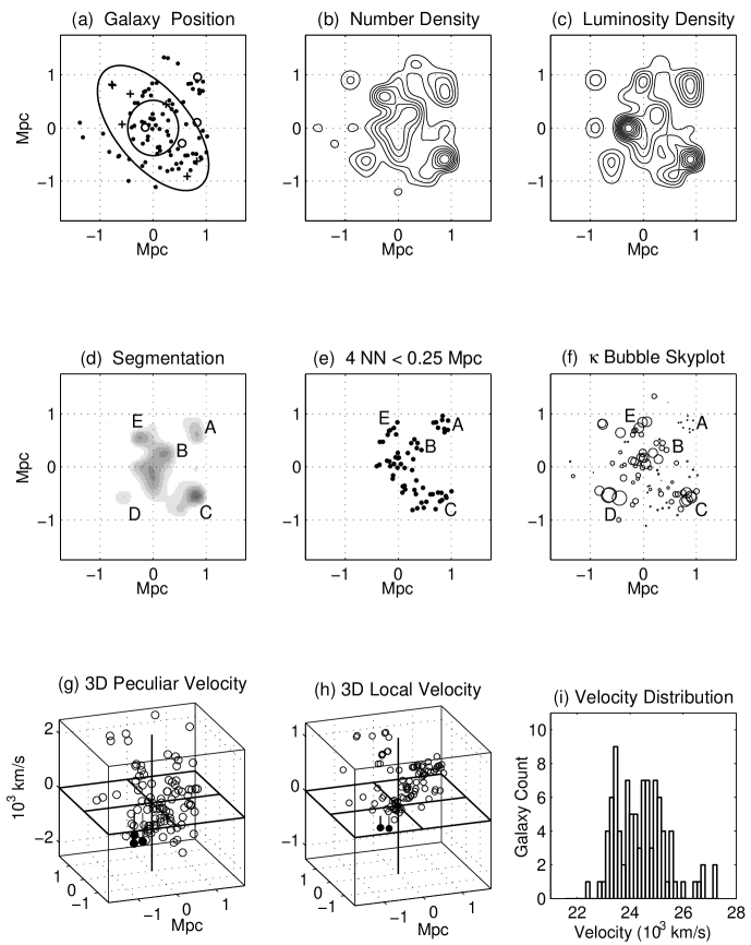
Figure 23: Visualization plots for Abell 1620.

At a distance of $d_{p}(t_{e})=231\,h^{-1}\,\mathrm{Mpc}$, Abell 1620 is one of the most distant clusters in this study. Inspection of Abell 1620 2D plots (Figures 23(a)–(e)) reveals an irregularly-shaped, low-density central region with four distinct groupings outside the central region labeled A, C, D, and E with a fifth possible subcluster just northwest of the core labeled B. Groupings A and C possess maximum number densities equivalent to that of the central region, $\sim 60\,\mathrm{gal}/(h^{-1}\,\mathrm{Mpc})^{2}$. Groupings D and E are less prominent with densities of $\sim 30-40\,\mathrm{gal}/(h^{-1}\,\mathrm{Mpc})^{2}$.

The central regionof the cluster show almost no ellipticity at a mean radius of 0.5 $h^{-1}$ Mpc, but are moderately elliptical with $\epsilon=0.49$ at a mean radius of $0.75\,h^{-1}\,\mathrm{Mpc}$ as grouping B influences the computation. At mean radii of 1.0 $h^{-1}$ Mpc, the ellipticity is still around $\epsilon$ = 0.50, but there is a position angle change due to the influence of C and E. Overall, the position angles maintain a fairly narrow range at all mean radii, ranging from $PA$ = 17^∘ to 41^∘, in approximate alignment with E, the core, and C with the exception of the $0.5\,h^{-1}\,\mathrm{Mpc}$. The core parameters are computed using the average ellipticity and position angle to yield a mean core radius of $R_{c}=0.47\pm 0.02$ and a central density of $\sigma_{0}=59\pm 3$ gal/($h^{-1}$ Mpc)² indicating the relatively diffuse nature of the central region.

The velocity distribution is skewed toward higher velocities (Figure 23(i)) resulting in a skewness value of $S=0.77=1.9\sigma_{S}$. The distribution is also somewhat broad compared to a Gaussian with $K=0.65=0.6\sigma_{K}$. The $\chi_{vel}^{2}$ test rejects the hypothesis of normality at the 97% CL.

The $\beta$ test for asymmetry indicates a very high probability of substructure with a $P_{\beta}\approx 0.1\%$. While the subgroups are somewhat evenly distributed around the centre, the density of the subgroups is significantly different, causing the computed high asymmetry value.

The 3D $\kappa$ test indicates a high probability of substructure with a $P_{\kappa}=0.9\%$. As seen in Figure 23(f), the level of $\kappa$ is relatively high in the core, and subgroups C, D, and E. The absence of significant $\kappa$ in A can be explained by the similarity of A’s local velocity distribution relative to the global cluster velocity distribution: the mean velocity of A is 24,486 km/s compared to 24,430 km/s for the cluster, and the related dispersions are 1103 km/s and 1001 km/s. Also note the presence of significant $\kappa$ in the (projected) central region that may indicate the presence of an additional subcluster or substructure.

4.6 Abell 1663

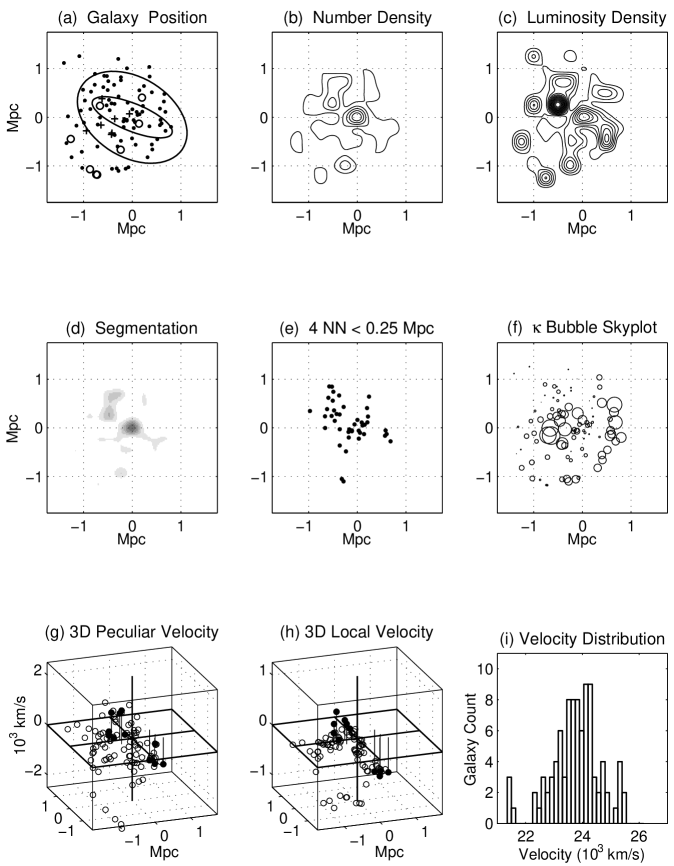
Figure 24: Visualization plots for Abell 1663.

Surface plots of Abell 1663 (Figures 24(a)-(e)) reveal a large, low density, bimodal central region. The centroid calculation used here is biased by the (projected) bimodal structure region so that the centre is re-positioned to be coincident with the peak number density. The northeast component contains the most luminosity for this particular cluster sample.

Three galaxies are questionable cluster members. The second brightest galaxy in the cluster is also the slowest galaxy in the cluster (2.9$\sigma$ from the mean) and on the periphery of the cluster (1.4 $h^{-1}$ Mpc from the centre at coordinates ($-0.72$, $-1.18$)). The other two galaxies are not overly bright ($b_{J}$ = 18.6 and 18.7), but are very close to the bright galaxy in both space (within 0.19 $h^{-1}$ Mpc) and velocity (within 350 km/s). This proximity suggests a bound group of three galaxies that, based upon the spatial, velocity, and luminosity data, is probably not associated with this cluster. As their influence on the statistical tests is negligible, it does not matter if these three galaxies are included or removed from the cluster sample.

Compared to the other clusters in the study, Abell 1663 is moderately elliptical with a position angle biased by the presence of the subcluster to the northeast (see Table 2). The core parameter values of $R_{c}=0.46\pm 0.03$ and $\sigma_{0}=57\pm 4$ are computed using the ellipticity parameters for the 1.0 $h^{-1}$ Mpc ellipse that improves the fit in this region compared to the circular fit while degrading the fit in the outer regions.

The velocity distribution is skewed toward lower velocities resulting in a skewness statistic of $S=-0.60=1.5\sigma_{S}$ with a kurtosis of $K=0.86=0.8\sigma_{K}$ (also see Figure 24(i)). However, the $\chi^{2}_{vel}$ test indicates this distribution is indistinguishable from a normal distribution with only a 36% CL to reject the normality hypothesis.

With the re-positioning of the cluster centroid, the $\beta$ test then yields a marginally significant result of $P_{\beta}=4\%$. However, the strong indication from the $\kappa$ test of $P_{\kappa}=0.1\%$ together with inspection of the bubbleplot in Figure 24(f) seems to indicate additional substructure beyond the apparent bimodality. Two subclusters are evident in the 3D plots (Figures 24(f)-(h)). One appears slightly east of the centre and the other approximately 0.8 $h^{-1}$ Mpc west of the centre. The subcluster nearest the centre is in very close proximity to but not actually part of the bimodal central region. With the faster subcluster east of the centre and the slower subcluster west of the centre, the velocity gradient is a possible signature for cluster rotation or infall dynamics, but further analysis is required for an accurate determination. The $\kappa$ bubble plot (Figure 24(f)) also shows another possible subcluster approximately 1.0 $h^{-1}$ Mpc due south of the centre.

4.7 Abell 1750

With a mean redshift of $z=0.086$, Abell 1750 is one of the more distant clusters in this study ($d_{p}(t_{e})=232\,h^{-1}\,\textrm{Mpc}$), and the present sample comprises 78 measured redshifts. It has been investigated for substructure in both the galaxy distribution and intracluster X-ray emission by Forman et al. (1981), Quintana & Ramirez (1989), Ramirez & Quintana (1990), Beers et al. (1991), West, Jones & Forman (1995), Bliton et al. (1998), Jones & Forman (1999), and Donnelly et al. (2001). Overall, our results are consistent with these previous studies although we do find some differences described below.

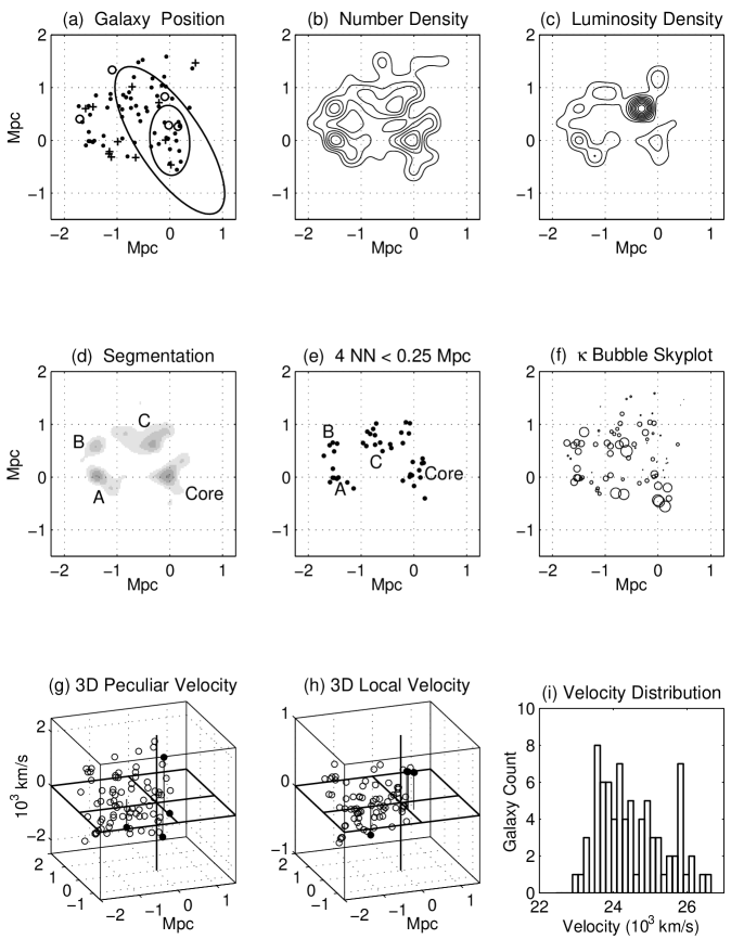
Figure 25: Visualization plots for Abell 1750.

The cluster shows two prominent galaxy concentrations in both the galaxy and the X-ray distributions. In the following analysis, the cluster center is set to be coincident with the peak X-ray emission (labeled as Core in Figure 25) although the number density in the C subgroup is comparable (and the visual comparison between the two is affected by binning). Fitting any smooth profile over the extent of this cluster is problematic due to the clumpy nature of the galaxy distribution. For the Core region, the elliptical King fit yields the smallest value in this sample for the central density of only $41\pm 4\;\textrm{gal}/(h^{-1}\,\textrm{Mpc})^{2}$. At mean radii greater than $\gtrsim 0.50\,h^{-1}\;\textrm{Mpc}$, the ellipticity calculation is heavily biased by galaxies to the north and northeast of the core region (see Figures 25(a)-(d)).

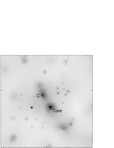
Figure 5: ROSAT PSPC image of Abell 1750 showing the two major components are associated with X-ray emission indicative of bound clumps. The brightest cluster member is located near the peak of the C subcluster emission.

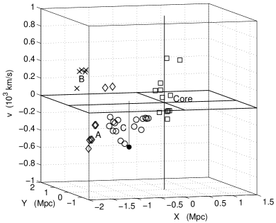
Figure 6: Local velocities of the nearest neighbors in Figure 25(e) for Abell 1750. In this plot, the Core galaxies are marked by squares, the A galaxies by diamonds, the B galaxies by crosses, and the C galaxies by circles.

The clumpiness in the projected surface density is especially evident in Figures 25(d)-(e) where at least 3 potential subclusters are indicated by labels A, B, and C with the C grouping possibly possessing additional structure. The Core and C grouping correspond to the SW and NE subclump of Donnelly et al. (2001). The other clumps identified here have no corresponding structure in the X-ray maps presented by Donnelly et al. or in the ROSAT PSPC X-ray map of Figure 5. The peak luminosity for this cluster sample is found in subcluster C due to the presence of a single bright galaxy approximately 1.0 Mpc northeast of the centre. The X-ray emission to the southeast of the core region has no counterpart in the galaxy distribution in the current catalogue.

In addition, the velocity histogram in Figure 25(i) shows an additional velocity component corresponding to $cz\sim 27,000$ km/s that is not present in the Donnelly et al. data. The hypothesis that the velocity distribution for Abell 1750 can be drawn from a normal distribution can be rejected at greater than the 98% CL (Table 4).

Quantifying the highly asymmetric visual and clumpy appearance of the distribution of galaxies on the sky, the $\beta$ test indicates that substructure is present at the $<0.1\%$. The higher order $\kappa$ test (Figure 25f) also shows distinct signs of substructure with relatively clear evidence for the Core, A, B, and C subclusters ($P_{\kappa}\,<\,3\%$). This test reveals that that both the Core and C regions seen in the number density map may be composed of 2-3 units. There is some evidence for this in the Xray map of Figure 5 for C, but the Core shows no obvious substructure in this figure. Further support for subclustering is revealed by the plot of local velocities of the nearest neighbors shown in Figure 6 where again the Core galaxies may possibly break into smaller clumps separated in local velocity by $\sim 180\,\mathrm{km/s}$, and with clear identifications for the A, B, and C subclusters.

Overall, the results above are consistent with previous X-ray results that Abell 1750 is at least a triple system (Jones & Forman, 1999). The velocity data presented in Beers et al. (1991) reveal that this system is even more complex with at least four components of which the subclusters labeled as Core and D here appear to be gravitationally bound and infalling. Further dynamical analysis similar to that presented in Beers, Geller, & Huchra (1982) and Beers et al. (1991) applied to the subclusters identified here will be presented in a future paper in order to confirm the conclusion in Beers et al. (1991) that the Core and C subclusters are gravitationally bound, and to ascertain whether any of the other subclusters are also bound components.

4.8 Abell 2734

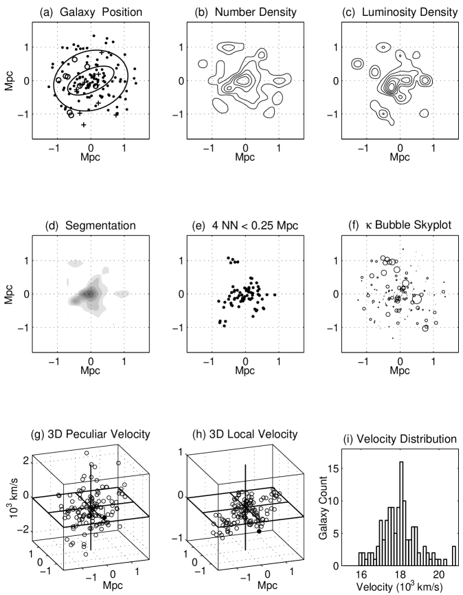
Figure 26: Visualization plots for Abell 2734.

Abell 2734 has a well defined, elongated core (see Figures 26(a) - (e)). With $\epsilon$=0.55, $PA$= 114^∘ with low to insignificant ellipticity at larger radii (Table 2). Comparison of the number density contours with the luminosity density contours, Figures 26(b) and (c), shows that the centre of luminosity is slightly offset from the number density centroid due to the position of the brightest galaxy in the catalogue of this cluster ($b_{J}=15.60$) at relative coordinates ($x=-0.14$ and $y=-0.23$). Further comparison of the position angle of the 0.5 $h^{-1}\,\mathrm{Mpc}$ ellipse with the luminosity density contours in Figure 26(c) reveals that the line connecting the centre of luminosity to the cluster centroid is approximately parallel to the position angle of the dispersion ellipse. The core parameters are $R_{c}=0.31\pm 0.01\;h^{-1}\,\mathrm{Mpc}$ with a maximum density $\sigma_{0}=121\pm 5\;\mathrm{gals}/(h^{-1}\,\mathrm{Mpc})^{2}$, and where the elliptical fit of the core parameters provides a noticeably better representation of the inner regions compared to the circularly symmetric fit.

Inspection of the redshift distribution shows the presence of three galaxies with redshifts close to $cz=22,000km/s$. Each of those three are possible background galaxies, but only one has a magnitude that makes it an obvious non-member candidate. These three galaxies have an insignificant influence on the computation of the velocity statistics that yields relatively high values for the skewness and kurtosis of $S=0.71\;\mathrm{and}\;K=1.38$. These values are $2.1\sigma\;\mathrm{and}\;1.6\sigma$, respectively, away from the expected value for a normal distribution (see Table 4). However, the $\chi^{2}_{vel}$ test yields an insignificant $85\%$ CL that the distribution can be rejected as normal.

Of the four statistical tests, the 2D $\beta$ test yields the strongest indication of structure/substructure with the computed asymmetry having a probability of random occurrence of only $P_{\beta}=0.4\%$. Closer examination reveals this asymmetry is caused by what appears to be a chance distribution – the mirror image of a relatively isolated galaxy happens to fall within a small group of galaxies. The member with the highest $\beta$ statistic is located near coordinate ($0.5$, $-1.0$). Its mirror image at coordinate ($-0.5$, $1.0$) is located close to a group that also exhibits substructure in the $\kappa$ test (see below). Other mirror images with high $\beta$ statistics do not fall in groups with any appreciable 3D structure, suggesting these groups may be the result of projection. If so, the positive $\beta$ test result could be a false positive.

With $P_{\alpha}=44.8\%$ and $P_{\kappa}=35.3\%$, the 3D tests show no significant indication of dynamical substructure. However, the $\kappa$ bubble skyplot in Figure 26(f) shows a small subcluster in the northeast at approximate coordinates ($-0.4$, $1.1$), and possibly some structure in the core. The structure in the core could be a merger signature, but more detailed examination is required to be certain.

Prior substructure studies of this cluster found similar results. Solanes, Salvador-Solé, & González-Casado (1999), using 45 members with redshift data, found no substructure ($P_{S}$ = 28.3%, $P_{K}$ = 41.5%, $P_{\Delta}$ = 14.0%). Kolokotronis et al. (2001) found weak or no substructure activity comparing optical and X-ray surface brightness parameters ($\epsilon$, $PA$, and centroid shift, $sc$). Biviano et al. (2002), using 77 members with redshift data, found no substructure with the $\Delta$ test ($P_{\Delta}$ = 10.0%). The $\Delta$ test result for our sample is $P_{\Delta}=38\%$ (see Vick 2004).

4.9 Abell 2814

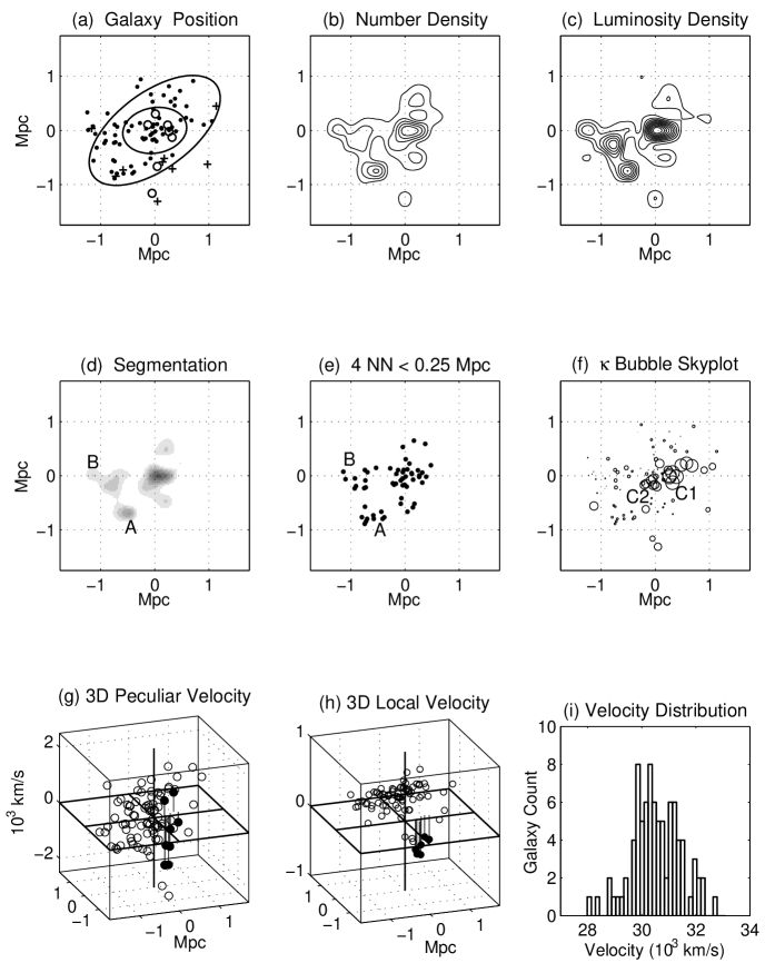
Figure 27: Visualization plots for Abell 2814.

At a distance of $d_{p}(t_{e})=284\,h^{-1}\,\mathrm{Mpc}$, Abell 2814 is the most distant cluster in this study. Figures 27(a)-(b) reveal an irregularly-shaped cluster possessing a relatively well-defined core region with isolated lower density concentrations of galaxies well removed from the central regions to the east and southeast labelled as groupings A and B in Figures 27(d)-(e). A few, possibly isolated, galaxies to the north and south are also present but do not appear to form subgroupings. Comparison of Figures 27(b) and (c) show that the luminosity density distribution is very similar to the number density distribution with most of the light emanating from the central regions.

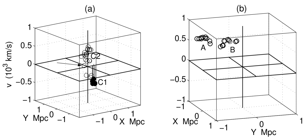
Figure 7: Local velocities of the nearest neighbors for Abell 2814 in Figure 27(e). For visualization purposes, only the galaxies in the (projected 2D) core are shown in (a) with the brightest cluster galaxy indicated by the arrow, while only the galaxies in groupings A and B are shown in (b).

The ellipticity and position angle of the $0.5\,h^{-1}\,\mathrm{Mpc}$ mean radius ellipse are $\epsilon=0.30$ and $PA=100^{\circ}$ with the position angle connecting the centres of the regions marked C1 and C2. Due to the galaxies to the north and south becoming included in the ellipticity computation, the position angle shifts by $30^{\circ}$ for the $0.75\,h^{-1}\,\mathrm{Mpc}$ ellipse ($\epsilon=0.27$ and $PA=130^{\circ}$) At larger mean radii, the galaxies to the east and southeast again increase the ellipticity while the position angle does not change appreciably (see Table 2). In fitting the core parameters, the circular fit does well with the outer regions while using the ellipse parameters for the $0.5\,h^{-1}\,\mathrm{Mpc}$ ellipse provides a noticeably better fit to the inner regions, yielding values of $R_{c}=0.36\pm 0.01\,h^{-1}\,\mathrm{Mpc}$ and $\sigma_{0}=81\pm 4\,\mathrm{gal}/(h^{-1}\,\mathrm{Mpc})^{2}$.

The velocity distribution shown in Figure 27(i) appears relatively normal, and the $\chi^{2}_{vel}$ test gives an insignificant 68% CL to reject the normality hypothesis. Similarly, the skew and kurtosis show relatively small deviations from normal values (see Table 4).

Due to the asymmetry introduced by the concentrations to the east and southeast, the $\beta$ test gives a $P_{\beta}=8\%$ chance of random occurrence. The three-dimensional $\alpha$ and $\kappa$ tests yield $P_{\alpha}=1.3\%$ and $P_{\kappa}=6.5\%$ probabilities of random occurrence, respectively. However, the results from these latter two tests are influenced not by the potential substructure in the eastern and southeastern concentrations as much as by a potential subcluster of at least eight galaxies just west of the cluster centre labelled C1 (see Figures 27(f) and (h)). As can be seen from the plot of nearest neighbor local velocities in Figure 7(a), the groups of bubbles in Figure 27(f) labeled as C1 and C2 appear as a distinct clumps with a few remaining galaxies in the projected (2D) core not appearing to clump together. The brightest cluster galaxy resides near the centre of the position-local velocity space. These isolated galaxies may reside outside the core region in 3D space. Whether C1 is a subcluster in or near the core itself or is in the foreground remains to be determined, but the structure does indicate probable infall/merger dynamics. From Figure 7(b), the groupings A and B are also probable subclusters.

4.10 Abell 3027/APM 268

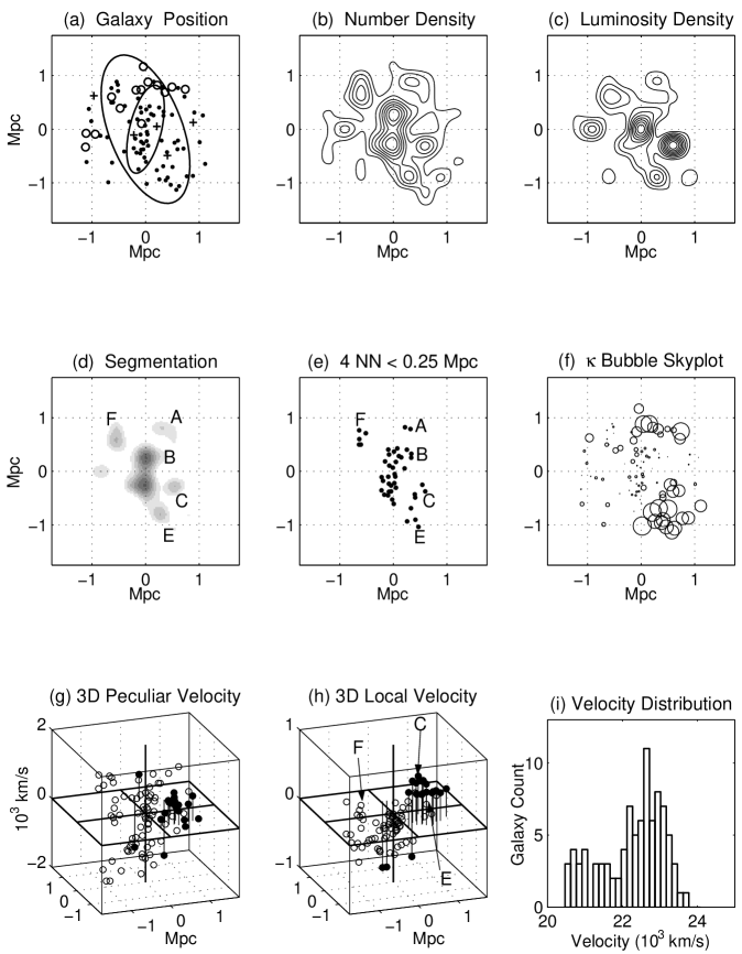
Figure 28: Visualization plots for Abell 3027.

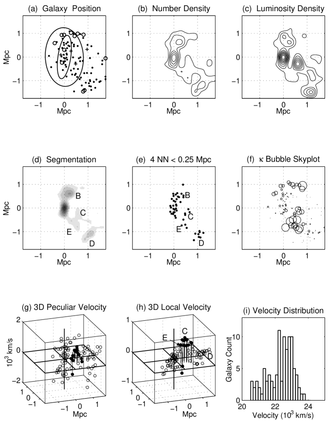
Figure 29: Visualization plots for APM 268.

Abell 3027 and APM 268 are essentially the same cluster with the primary differences in the 2dFGRS catalogue being some galaxies to the east and northeast included in A3027 are not included in APM268, and some galaxies to the southwest that are included in APM268 but not included in A3027 (see Figures 28(a) and 29(a)). The central regions are similar but not identical, leading to small but noticeable differences in the number and luminosity density contour plots, Figures 28(b), (c) and 29(b), (c). Analysed together, these two clusters present an interesting test case for checking the sensitivity of the various algorithms to small differences in cluster membership.

The surface plots for A3027 indicate the central region may consist of two components of approximately equal galaxy density, but this is not as evident in the plots for APM268. With the centre of luminosity residing at the computed origin in both cases due to the brightest cluster member ($b_{J}=15.75$), no center re-positioning was done (see Figures 28(c) and 29(c)). An X-ray map of this cluster would be useful in determining the central region distribution. The elongated (or bimodal) central structure biases the ellipticity computation to yield high ellipticities with position angles oriented north to south for mean radii out to $\sim 0.75$ Mpc at which point the galaxies in the outer region become included and reduce the calculated ellipticity values (see Table 2). Using the ellipticity and position angle of the 0.75 Mpc mean radius, the core parameters are computed to be $R_{c}=0.29\pm 0.01$ and $\sigma_{0}=90\pm 3$ for A3027 and $R_{c}=0.30\pm 0.01$ and $\sigma_{0}=81\pm 3$ for APM268.

Four groupings of galaxies outside the core are common to both clusters, and are marked as A, B, C and E in Figures 28(d) and 29(d). A concentration to the northeast in Abell 3027 is marked as F in Figure 28(d), and a concentration to the southwest is marked as D in Figure 29(d). Grouping C contains the second brightest galaxy in this sample ($b_{J}=16.08$) so that the luminosity density is only slightly less than in the core.

Inspection of the velocity histograms in Figures 28(i) and 29(i) hint at superpositions of distributions that considered as a single entity is clearly not normal. The $\chi^{2}_{vel}$ test rejects the hypothesis of a single normal distribution at greater than the 99.9% CL and $98\%$ CL for APM268. The galaxies in the north contribute most of the slower galaxies (marked by the open circles in Figures 28(a) and 29(a)), and the distribution centered at $\sim 23,000\,\mathrm{km/s}$ resulting from eliminating galaxies with velocities less than $\sim 22,000\,\mathrm{km/s}$ is decidely more gaussian-shaped.

The $\alpha$ and $\beta$ tests yield no significant substructure for A3027 but do for APM268 (Table 6). With $P_{\kappa}=0.2\%$ and $2.2\%$, the $\kappa$ test does show strong indications of substructure. The slower galaxies to the north have relatively large bubbles, but do not appear to be part of any organized structure, and may be in the foreground, and grouping A does not appear to be a 3-dimensional structure. Grouping B, just outside the core region, does not show significant $\kappa$, but does show some separation from the core in Figures 28(f) and 29(f). However, groupings C and E show significant $\kappa$ and are possible subclusters. Groupings D and F do not show a large amount of $\kappa$, but appear in the local velocity plots of Figures 28(h) and 29(h) (along with C and E), and may be subclusters with dominant galaxy motions tranverse to the line-of-sight, or subclusters with similar velocity distributions to the core region. Overall, A3027/APM268 shows substructure in the core and outer regions that should be further investigated through a detailed X-ray study.

Figure 8: Abell 3094 Velocity Distribution of (a) the East Group ($x<-0.60\,h^{-1}$ Mpc) and (b) the Other Cluster Members ($x>-0.60\,h^{-1}$ Mpc ).

Figure 9: Abell 3094 (a) 3D peculiar velocity, and (b) 3D local velocity plots with the outlier removed.

4.11 Abell 3094

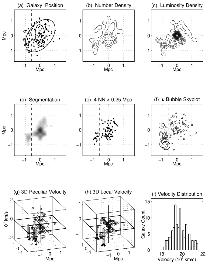
Figure 30: Visualization plots for Abell 3094.

The 2D plots in Figures 30 (a)-(e) show a cluster with an extended low density central region with two projected surface density peaks oriented north to south. Concentrations of galaxies with densities greater than $40\,\mathrm{gal}/(h^{-1}\,\mathrm{Mpc})^{2}$ appear 0.75 - 1.0 $h^{-1}$ Mpc to the east and north-northwest of the cluster centre. The luminosity contour plot has a similar shape as the high density regions in the isodensity contour plot, but without a bimodal central region (at the resolution shown here).

Due to the apparent bimodal central region, ellipticity at the smaller mean radii is noticeable with $\epsilon=0.55\,\mathrm{and}\,0.49$ at mean radii of 0.5 and 0.75 $h^{-1}\,\mathrm{Mpc}$, respectively. At mean radii of 1.0 to 1.25 $h^{-1}$ Mpc, the groupings to the east and north-northwest bias the ellipticity computation resulting in values of $\epsilon=0.37-0.33$ at postion angles of $PA\approx 140^{\circ}$. We use the $\epsilon$ and $PA$ for the mean radius of 1.0 $h^{-1}$ Mpc to compute a mean core radius $R_{c}=0.39\pm 0.01\,h^{-1}$ Mpc and a central density $\sigma_{0}=88\pm 2$ (Table 3).

The velocity distribution shown in Figure 30(i) is skewed toward higher velocities with $S=0.42$ ($1.15\sigma$ from normal) while the kurtosis is close to normal. The relatively high value of skewness is probably the primary cause that the $\chi^{2}_{vel}$ test rejects of the normal hypothesis at a 93% CL (Table 4).

The $\beta$ test indicates cluster asymmetry with a marginally significant $P_{\beta}$ = 10%, and the $\kappa$ test indicates a very high probability of substructure with $P_{\kappa}<0.1\%$. Most of the significant $\kappa$ in the core is associated with galaxies in the northern projected component. However, while the local velocity plot of the nearest neighbors in Figure 9(b) does indicate some spatial structure in the core, it is not entirely clear whether it should be classified as bimodal. Further inspection of the $\kappa$ bubble skyplot in Figure 30(f) shows that most members with a location of $x<-0.60h^{-1}$ Mpc have a relatively high $\kappa$ statistic. Analysis shows that this group, with the exception of one galaxy, has a significantly slower velocity distribution than the other members of the cluster with $x>-0.60\,h^{-1}$ Mpc (see Figure 8).

The mean velocity of the eastern grouping (not including the outlier) is 18,989 km/s or 898 km/s slower than cluster members to the west. The velocity dispersion of the eastern grouping is $\sigma_{vel}$ = 401 km/s, significantly smaller than the $\sigma_{vel}=662\,\mathrm{km/s}$ dispersion of the galaxies to the west (and $\sigma_{vel}$ = 728 km/s for the entire cluster). For ease of visualization, a dashed line is drawn on Figures 30(a)-(f) showing the approximate border of the eastern grouping. Ten of the 23 members in the east group show a $>5\%$ probability that the member and its nearest neighbors are not from the same distribution as the entire cluster. When the outlier is removed, the number of members with a $>5\%$ probability increases from 10 to 18. A possibility for shearing or infall motion is also more evident in the 3D plots with the outlier removed as shown in Figures 9(a) and (b).

In the substructure study of ENACS clusters, Solanes, Salvador-Solé, & González-Casado (1999) used 46 redshifts to compute a $\Delta$ test statistic of $P_{\Delta}$ = 0.4%, similar to that given in Biviano et al. (2002). These results are consistent with the value of $P_{\Delta}=0.4\%$ found by Vick (2004) and the $\kappa$ test result reported here for the sample of 108 2dFGRS redshifts. Other tests in the ENACS study were less conclusive.

In summary, Abell 3094 shows a high probability of substructure with the $\kappa$ test, and some indication with the $\chi^{2}_{vel}$ and $\beta$ tests (see Table 6). A grouping of 22 galaxies located east of $x=-0.60\,h^{-1}$ Mpc may represent a foreground group or a large subcluster with infall or possibly shearing motion.

4.12 Abell 3880

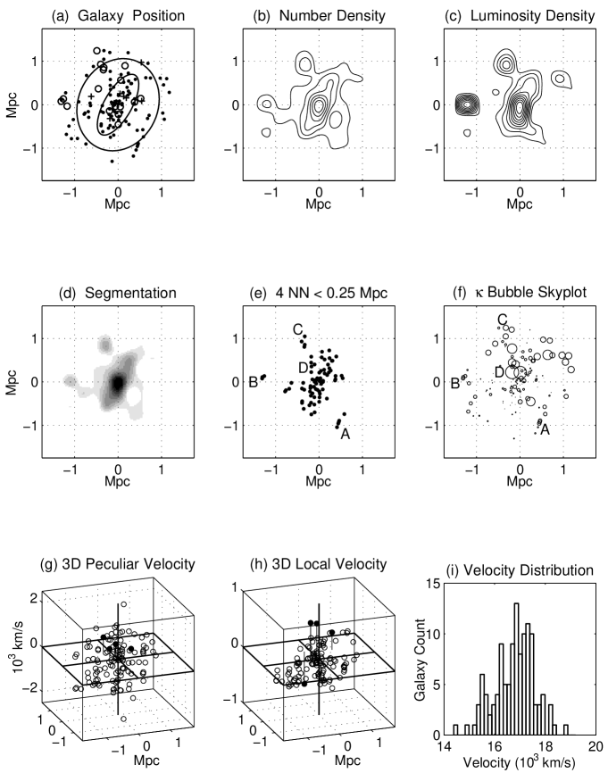
Figure 31: Visualization plots for Abell 3880.

Inspection of Figures 31(a)-(b) shows Abell 3880 as an elliptical cluster with a well-defined, dense core. Comparison of Figures 31(b)-(c) shows that the luminosity density of the core region closely traces the number density. From Figure 31(b), there are at least three potential subclusters(A, B, and C) with two having density greater than 40 galaxies per ($h^{-1}$ Mpc)², each of which is just over 1.0 $h^{-1}$ Mpc from the cluster centroid (see Figure 31(d)). Two of these groupings, A and B, show a relatively high level of luminosity (Figure 31(c)). This combination of high luminosity with slow peculiar velocity hints at possible foreground contamination; inspection of the velocity-magnitude plot reveals at least four galaxies as candidate, but not obvious, non-members.

Closer inspection of the three groupings shows each to contain five galaxies in close projected (2D) spatial proximity. In particular, grouping B contains the brightest galaxy in this sample ($b_{J}=14.69$) with a velocity a little more than $1.3\sigma$ away from the cluster mean (one of the non-member candidates mentioned above). Of the remaing four galaxies in grouping B, two have velocities very similar to the brightest galaxy, $\approx 1050\;\mathrm{km/s}$ less than the cluster mean, while the other two have velocities $\approx 365$ km/s greater than the cluster mean. Thus, it is possible that grouping B consists of a foreground group of three galaxies with projected surface positions close to two cluster members. Grouping C is similar to B in that of the five galaxies, one is relatively bright ($b_{J}=15.45$) with a velocity more than 1200 km/s less than the cluster mean, two others have similar velocities, while the remaining two have velocities more than 300 km/s greater than the cluster mean. Finally, grouping A possesses relatively low luminosity, and consists of three galaxies having velocities close to the cluster mean and two galaxies having velocities 705 and 917 km/s faster than the mean.

Corresponding to the elongated contours tracing the central regions, the ellipticity is relatively high for the $0.50\;\mathrm{and}\;0.75\;h^{-1}$ Mpc ellipses with $\epsilon=0.59\;\mathrm{and}\;0.50$ at position angles of $PA=150^{\circ}\;\mathrm{and}\;159^{\circ}$. As the mean radius is increased to 1.0 $h^{-1}$ Mpc, the ellipticity decreases to a relatively low value ($\epsilon=0.16,PA=156^{\circ}$) due to the influence of the three high density areas outside the core. To reduce the influence of the groupings in the determination of the core parameters, the ellipticity and position angle are averaged for the $0.75\;\mathrm{and}\;1.0\;h^{-1}$ Mpc mean radii to yield best fit parameters of $R_{c}=0.25\pm 0.01\;h^{-1}$ Mpc and $\sigma_{0}=161\pm 13\;\mathrm{gal}/(h^{-1}\;\mathrm{Mpc})^{2}$ (a relatively high value for the central density). The resulting elliptical fit to the density profile is noticeably better than the circular fit in the inner regions of the cluster.

Other than the three groupings described above, there is little obvious substructure present in this cluster. The statistical $\alpha$, $\kappa$, and $\chi^{2}_{vel}$ yield results for substructure below the 90 % CL. However, it is worth noting that the nearest neighbor plot and the $\kappa$ bubble skyplot indicate that a fourth grouping of at least five galaxies, marked D in Figure 31(e), is also a possible subgroup (and might be detectable in a long exposure X-ray observation). Stein (1997) initially considered but rejected A3880 for investigation due to there being less than 25 galaxies within $0.5\,h^{-1}\,\mathrm{Mpc}$ of the centre in the catalogue used for that study; in the study here, there are $\sim 45-50$ galaxies within a $0.5\,h^{-1}\,\mathrm{Mpc}$ circle or dispersion ellipse. However, Stein quotes a mean cluster velocity and dispersion for the core galaxies consistent with what is found here.

4.13 Abell 4012

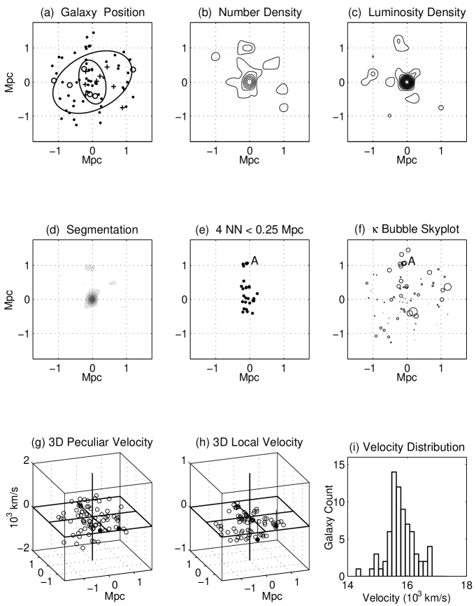
Figure 32: Visualization plots for Abell 4012.

Abell 4012 has a low-density core with one obvious subgrouping of galaxies approximately $1.0\,h^{-1}$ Mpc due north of the centre with a density exceeding 40 gal/($h^{-1}$ Mpc)² (see Figures 32(a), (b)). These five galaxies in the northern grouping are marked as A in Figure 32 and are discussed further below (two galaxies have nearly coincident angular positions and are indistinguishable in the plots).

At small mean radii, the cluster has a moderate level of ellipticity that decreases to insignificance at the larger mean radii (Table 2). At a mean radius of 0.5 $h^{-1}$ Mpc, $\epsilon=0.42$ with $PA=14^{\circ}$ where the position angle points directly toward Abell 4013. By a mean radius of 1.25 $h^{-1}$ Mpc, the ellipticity is negligible ($\epsilon$ = 0.01, $PA$ = 133^∘). Compared to a circular fit, the elliptical fit is noticeably better with a mean core radius of $R_{c}=0.28\pm 0.01h^{-1}$ Mpc and $\sigma_{0}=71\pm 3$ galaxies/$(h^{-1}\mbox{Mpc})^{2}$.

With a value of $\sigma_{vel}=471$ km/s, the velocity dispersion is one of the smallest found in this study (Table 4). Inspection of the velocity distribution in Figure 32(i) shows what appears to be a somewhat normal distribution. The skewness and kurtosis values of $S=-0.08$ and $K=0.37$ are each less than $0.5\sigma$ from what is expected for a normal distribution (see Table 4). However, the $\chi^{2}_{vel}$ test shows a 96% confidence level to reject the normal distribution hypothesis.

Inspection of Figures 32(a)-(e) shows the only clear sign of subtructure as the previously mentioned small clump of galaxies to the north of centre. However, consisting of only five galaxies, this grouping is not enough to cause the $\beta$-statistic to indicate significant asymmetry ($P_{\beta}=26\%$).

The $\alpha$ test indicates substructure ($P_{\alpha}=1$% probability of random occurrence) but the $\kappa$ test does not ($P_{\kappa}=21$%). In order to better isolate any apparent dynamical clumpiness in this cluster, the nearest neighbor positions in Figure 32(e) are displayed in a local velocity plot in Figure 10. This plot clearly shows the grouping A to be a probable bound subcluster. If this interpretation is correct, the local gravitational potential minimum should be detectable in a long exposure X-ray observation. The other hints of clumpiness in Figure 32(e) are not as clearly manifested in Figure 10, but cannot be completely excluded as small subclusters or merger remnants.

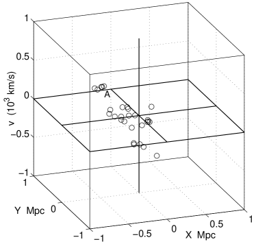
Figure 10: Local velocity plot of the nearest neighbor positions for Abell 4012 shown in Figure 32(e).

4.14 Abell 4013

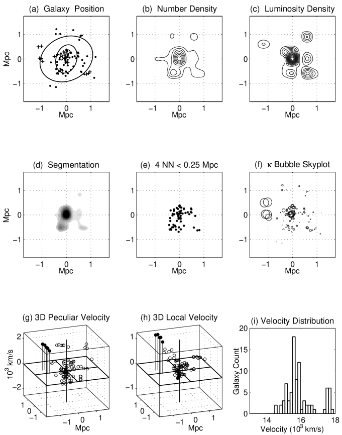
Figure 33: Visualization plots for Abell 4013.

Inspection of Figures 33(a),(b), and (d) shows a cluster with a well-defined, dense core. Approximately 0.5 $h^{-1}$ Mpc south of the cluster centre is an additional high density group of galaxies having a peak density of greater than 60 gal/$(h^{-1}\mbox{ Mpc})^{2}$. Two small groupings appear west and southwest of the centre. For this cluster, the luminosity density is very similar to the number density (compare Figures 33(b) and (c)).

Within the $0.5\,h^{-1}\mbox{ Mpc}$ dispersion ellipse, the values of $\epsilon$ = 0.29 and $PA$ = 163^∘ are biased by the high-density group of galaxies to the south. The ellipticity decreases at larger radii as the influence of this high-density subcluster decreases. At a mean radius of 1.0 $h^{-1}$ Mpc, $\epsilon$ = 0.20 with a $PA$ = 116^∘. The core fit yilds a core radius of $R_{c}=0.17\pm 0.01$ and a maximum density of $\sigma_{0}=224\pm 2\,\mathrm{gal}/(h^{-1}\,\mathrm{Mpc})^{2}$. The resulting fit accurately reproduces the density profile for most of the cluster. The $\beta$ test indicates substructure at high significance with $P_{\beta}=2$% where the high level of asymmetry is caused by the southern subgroup coupled with the relative absence of galaxies to the north.

Inspection of the velocity histogram (Figure 33(i)) shows a group of fast galaxies well-separated from the rest of the distribution: the majority of the cluster members are grouped around a velocity of 15,600 km/s, but a small group of 14 are found near 17,600 km/s. This feature explains the $>$ 99.9% CL to reject the hypothesis that the distribution is normal. These faster galaxies are in three spatial locations, and can clearly be identified in Figure 33(a) (marked by ‘+’ symbols). Five galaxies are approximately 1.0 $h^{-1}$ Mpc east of the centre, six galaxies appear near the centre of the cluster, and three are approximately 1.0 $h^{-1}$ Mpc southwest of the centre.

The $\kappa$ test yields an indication of substructure at slightly greater than the 95% CL, but inspection of Figure 33(f) shows that the large southern subgroup has relatively small bubbles, possibly indicating any dynamical interaction between core and subcluster is perpendicular to the line of sight. The high velocity galaxies to the east with the large $\kappa$ bubbles are also relatively fainter than the majority of cluster members, and may be background galaxies. But there are also significant $\kappa$ bubbles in the core region that may indicate the merger or dynamical interaction of small subgroup(s)(here, spatially unresolved) as indicated by the presence of slow and fast galaxies in the core.

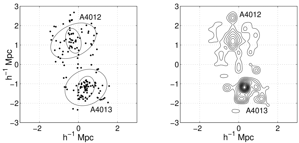
Figure 11: Relative galaxy positions and number density contours for Abell 4012 and Abell 4013.

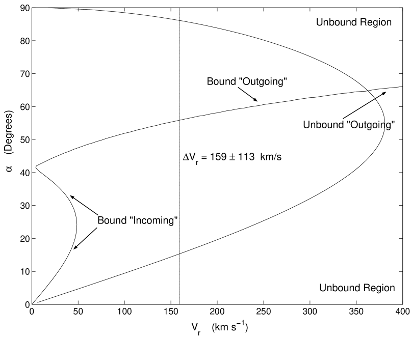
Figure 12: Bound and unbound solution space for Abell 4012 and 4013. A value of $H_{0}=70$ has been assumed for the solution of the parametric equations of motion. The angle $\alpha$ is a projection angle between the line-of-sight and the vector joining the two cluster centroids.

4.15 Abell 4012 and Abell 4013 as a possible bound system

It is worth noting the spatial proximity of these two clusters. The projected surface (2-dim) separation between the two centroids is $\approx 2.5\,h^{-1}$ Mpc, while their mean redshifts are $c\overline{z}=16,230\pm 498$ km/s and $c\overline{z}=16,410\pm 904$ km/s, respectively. Figure 11 shows the galaxy positions and number density contours from which it can be seen that the southern boundary of A4012 is relatively close to the northern boundary of A4013. Superimposed on the plot of galaxy positions are the $0.5\mbox{ and }1.0h^{-1}$ Mpc dispersion ellipses showing the approximate alignment of the inner regions of the two clusters.

Given their proximity, it is worthwhile assessing the likelihood that the two clusters are gravitationally bound to one another. The cluster masses are estimated using the virial relation

$$M_{vir}=\frac{N}{G}\sum_{i}v_{i}^{2}\left(\sum_{i}\sum_{j<i}\frac{1}{r_{ij}}\right)^{-1}\;\mbox{,}$$ (26)

where $N$ is the number of cluster members, $v_{i}$ is the peculiar velocity of the $i^{th}$ member, and $r_{ij}$ is the projected separation between the $i^{th}$ and $j^{th}$ galaxies. Inspection of the velocity distribution for Abell 4013 reveals 14 galaxies with velocities significantly faster than the other 71 members, and these are removed in the following analysis in order to minimize their effect on the velocity dispersion (see Figure 33(i)). Thus, we estimate the mass of Abell 4012 to be $\approx 7\times 10^{13}\mathrm{M}_{\bigodot}$ with a velocity dispersion of $\sigma_{vel}=471$ km/s, and a mass of $\approx 4\times 10^{13}\mathrm{M}_{\bigodot}$ for Abell 4013 with a velocity dispersion of $\sigma_{vel}=455$ km/s based on eliminating the “fast” galaxies. Using the Newtonian binding criterion

$$V_{r}^{2}R_{P}\leq 2GM_{tot}\,\sin^{2}\alpha\,\cos\alpha\;\;\mbox{,}$$ (27)

and the parametric analysis described in Beers, Geller, & Huchra (1982) for these masses, projection angle $\alpha$, projected centroid separation, and a radial velocity difference of $V_{r}=159$ km/s, we find a $\sim 95\%$ probability that A4012 and A4013 form a bound system with a less than $10\%$ probability for the bound ‘incoming’ solutions. The probability calculation is based primarily on the possible deviation of the actual radial velocity separation being different from the $V_{r}=159$ km/s value assuming no worse than a $113\,\mathrm{km/s}$ RSS measurement error. From Figure 12, the system is bound as long as $V_{r}$ is accurate to within 200 km/s where the parametric solutions indicated in the figure follow the terminology in Beers, Geller, & Huchra (1982).

4.16 Abell 4038

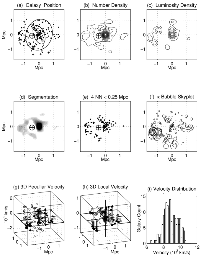
Figure 34: Visualization plots for Abell 4038.

Abell 4038 is a fairly rich cluster of richness class $\textrm{R}=2$, and we present analysis based on 154 galaxies in this system (the most of any cluster in this study). The core of this cluster is well defined with a central density of $\sigma_{0}=261\pm 15$ and fitted optical core radius of $R_{c}=0.19$ Mpc. To the east of the core, a dearth of galaxies can be seen in the galaxy distribution (Figure 34(a)) at ($-0.5$, $-0.1$) Mpc. This is also evident in Figures 34(b),(d), and (e). This apparent gap in the distribution is caused by the bright star (SAO 192167, $m_{v}$=4.6) which limits spectroscopy in the vicinity. The location of the star and a very approximate bounding area inside which galaxy identification is probably unobtainable are indicated by the (circle + cross) in Figures 34(a),(b),(d) and (e). From these figures it can be seen that while the blanking area covered by the star represents a substantial fraction of the gap area, there are still portions to the north and south that are clearly devoid of galaxies. If the gap is not real, one expects to see galaxies just outside the blanking area, so that it appears that at least part of the galaxy-free region is a true feature of the distribution. But it should be noted that the inability to detect cluster members in the vicinity of SAO 192167 could significantly bias the results of any substructure tests using the global cluster galaxy distribution on the sky if, in fact, cluster members are not being included. However, substructure tests that evaluate local parameters or the velocity distribution should be less affected.

Not surprisingly, the gap in the galaxy distribution strongly affects the analysis of this cluster including the ellipticity computation. Looking at the smallest radius of 0.5 h^-1 Mpc, the void has a strong influence on the ellipticity by cutting off the distribution on the east side. This results in a relatively large ellipticity of 0.43 and a position angle of $21^{\circ}$. At the largest radius the ellipticity has risen to 0.50 and the postion angle has moved to $96^{\circ}$. This is due to the apparently disjoint galaxy clump at ($-1.5$, 0) Mpc and the transition would possibly be more gradual without the data gap.

The $\alpha$ and $\beta$ tests indicate the presence of strong substructure. Since these two tests are more heavily influenced by the global distribution of galaxies on the sky, the gap in the galaxy distribution biases the results of these tests. The $\kappa$ test also indicates the presence of substructure with a very high significance but since this is a local test, it should be less influenced by the gap in the data. However, the absolute significance of the test needs to be investigated in more detail for this cluster.

The bubble plot in Figure 34(f) shows at least four areas with evidence of substructure. The most obvious are two groupings $\sim-1.2$ Mpc to the east, and separated from the main cluster by the gap discussed above. However, these features show up in the velocity plots (Figures 34(g) and (h)), and are clearly at discrepant velocities compared to the main cluster. The next most discrepant grouping is to the south of the main cluster at ($-0.4$, $-1.0$) Mpc, but this grouping is only weakly apparent in the number or luminosity density plots. This subclump appears to be well separated from the main concentration, but may be affected by the gap near the bright star. One other subclump is located west of the centre. The clump at (1.0,0.0) Mpc shows up as a low-level contour in the number density map and also can be seen in the local velocity plot. There may be additional substructure just northeast of the core (see Figures 34(b)) and (d)).

Although the $\alpha$, $\beta$, and $\kappa$ tests yield strong signals for substructure, the $\chi_{vel}^{2}$ test rejects the normality hypothesis at only the 96% CL. Yet the velocity distribution as shown in Figure 34(i) does show hints of being a superposition of two (or more) distributions.

This cluster has been previously studied for substructure in the galaxy distribution by Girardi et al. (1997), Stein (1997), and Kriessler & Beers (1997), and using ROSAT X-ray data by Schuecker et al. (2001). However, these studies considered the central region of the cluster, and did not include the eastern extension that may or may not be associated. The velocity statistics and $\Delta$ test value are consistent with those found here for that region. The Kriessler & Beers study presents a contour plot of the central region significantly different in appearance from ours, and their KMM analysis identifies three modes that we are unable to resolve. However, a new study of this cluster in X-ray with longer exposure times should further clarify the true substructure and resolve the problematic constraints imposed by SAO 192167.

4.17 Abell S141

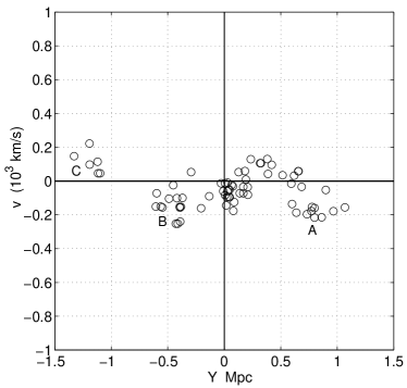
Figure 13: Nearest neighbor local velocities versus the y-coordinate for Abell S141. The apparent clumping in 2D also appears in 3D for at least groupings A, B, and C.

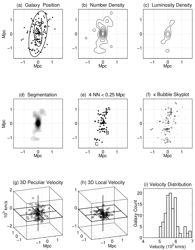
Figure 35: Visualization plots for Abell S141.

At a distance of $d_{p}(t_{e})=57\,h^{-1}\,\textrm{Mpc}$, Abell S141 is the nearest cluster in the study ($cz=5793\,\textrm{km/s}$). Inspection of Abell S141 2D plots in Figure 35 shows a highly elongated structure with two apparent clumpings in the south and possibly one in the north. The core is relatively dense, but, together with S1043, S141 has the lowest luminosity of the clusters studied here.

For the four mean radii from 0.5 to 1.25 $h^{-1}$ Mpc, the ellipticity and position angle have a narrow range from $\epsilon$ = 0.67 – 0.58 and $PA=0^{\circ}\,(\mathrm{or}180^{\circ})$ – $168^{\circ}$ (see Table 2). We use the average ellipticity of $\epsilon=0.64$ and position angle of $PA=173^{\circ}$ to calculate a core radius $R_{c}=0.26\pm 0.02$ and a central density $\sigma_{0}=158\pm 18$.

The velocity dispersion of $\sigma_{vel}=403\,\mathrm{km/s}$ for the distribution shown in Figure 35(i) is the lowest in this study. Also from this figure, it is evident that the distribution is skewed toward higher velocities due to the ten relatively fast members labelled with ‘+’ symbols in Figure 35(a). The $\chi_{vel}^{2}$ rejects the normality hypothesis at the 98% CL, but it is difficult to correlate the results of this test as due to any of the groupings except for possibly the one farthest south.

The three apparent subclumpings in the segmentation and nearest neighbor plots are labelled as A, B, and C in Figure 35(e). The local velocities of the nearest neighbors shown in Figure 13 appear to support the hypothesis that groupings B and C form subclusters with possibly also a fraction of grouping A forming a subcluster. However, the statistical tests yield no clear signal for substructure with the $\beta$ and $\alpha$ tests yielding $P_{\beta}$ = 23% and $P_{\alpha}$ = 34.6%. The lack of a signal in the $\beta$ test is easily explained from the obvious symmetry in the projected directions. The low velocity dispersion combined with the 2D symmetry is probably responsible for the lack of a signal from the $\alpha$ test.

Although the $\kappa$ test result of $P_{\kappa}=19.8\%$ using ten nearest neighbor velocities ($\approx\sqrt{N}$) is not statistically significant, there are some indications of subclustering in the bubble skyplot in Figure 35(f) corresponding to the groupings described above. Performing the $\kappa$ test with numbers of nearest neighbor velocities other than $\sqrt{N}$ did not appreciably change the significance level. However, for this cluster, the small dispersion of velocities naturally reduces the discriminating power of the test. This is probably due to the geometrical effects introduced from analyzing a cluster with one relatively long and two short symmetry axes along a direction perpendicular to the long axis. Thus, we conclude that in addition to the possible subclustering, the global shape of this cluster is triaxial with one long and two short axes (or possibly prolate). This geometry may be linked with the supercluster environment in which S141 formed.

4.18 Abell S258

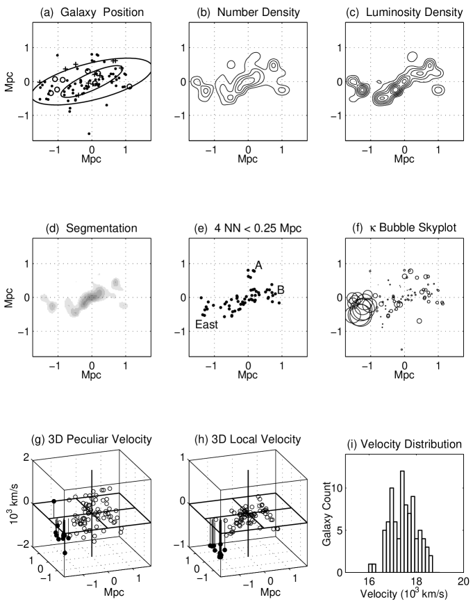
Figure 36: Visualization plots for Abell S258.

Abell S258 is highly elongated, as is evident upon viewing the 2D plots (Figures 36(a) - (e)). Its length stretches over 3 $h^{-1}$ Mpc in an east to west direction while its width is typically 1 $h^{-1}$ Mpc. It has a moderately dense central region that also appears highly elliptical in an east to west direction.

The ellipticity and position angle are very consistent for all mean radii with ranges of $\epsilon$ = 0.75 – 0.58 and $PA$ = $114^{\circ}$ – $104^{\circ}$ (see Table 2). This cluster has the highest ellipticity in the study at a mean radius of 0.5 $h^{-1}$ Mpc and the highest or second highest ellipticity at mean radii from 0.75 – 1.25 $h^{-1}$ Mpc. Using the ellipticity and position angle for the 1.0 $h^{-1}$ Mpc test radius ($\epsilon=0.71$, $PA=104^{\circ}$), we find a mean core radius, $R_{c}=0.28\pm 0.04$, and a maximum density, $\sigma_{0}=108\pm 1$ (Table 3).

The velocity distribution appears bimodal (see Figure 36(i)). This characteristic, however, is not sufficient to cause a negative test of normality as the $\chi^{2}_{vel}$ test rejects the normal hypothesis at an insignificant 70% CL (Table 4).

Only the $\kappa$ test indicates significant substructure (Table 6), but that test results in a very high significance level with a $P_{\kappa}<0.1\%$. Inspection of the $\kappa$ bubble skyplot (Figure 36(f)) shows a large number of members with a high level of $\kappa$ in the far eastern part of the cluster. Of the 14 members east of $x=-1.0\,h^{-1}$ Mpc, 12 are grouped very close in position and velocity. These 12 galaxies are found to have a much slower mean velocity ($\overline{v}$ = 16,863 km/s), are more narrowly dispersed ($\sigma_{vel}$ = 272 km/s) compared to the other members of the cluster ($\overline{v}$ = 17,584 km/s and $\sigma_{vel}$ = 526 km/s), and are responsible for the bimodal appearance of the velocity distribution. They can be seen clearly in the 3D velocity plots, Figures 36(g) and (h).

Table 5: Abell S258 Comparison of East and West Group.

	East Group	West Group	Cluster
N	12	75	87
$\overline{v}$	16,863 km/s	17,584 km/s	17,485 km/s
$\sigma_{vel}$	272 km/s	526 km/s	557 km/s
$\overline{b_{J}}$	18.0	18.0	18.0
$\chi^{2}_{vel}$	-	CL = 67%	CL = 70%

It is unclear if this eastern sublcluster is, in fact, part of Abell S258. It is possible that this group is a small foreground cluster. The eastern group has an average redshift of 767 km/s less than the remainder of the cluster which could equate to a foreground distance of 11 Mpc (using $h$ = .70). However, the velocity difference of 721 km/s is also within the range of possible orbital velocities estimated for a subcluster orbiting the main body. A binding probability analysis will be presented in a future paper. Comparing velocity versus magnitude for each member in each group is inconclusive in determining spatial separation. Moreover, removing the eastern group members did not significantly improve the likelihood for normality of the velocity distribution. Table 5 compares key statistics of each group and the cluster.

There are also possible subclusters to the west and north that are more readily apparent from inspection of the nearest neighbor plot, Figure 36(e), in which they are labeled ‘A’ and ‘B’. Subcluster B appears to contain eight galaxies grouped in both position and velocity space with other galaxies in the surface plot probably not being subcluster members. The northern A grouping appears to be a result of chance projection in the surface plots. Finally, the segmentation, nearest neighbor, and 3D local velocity plots suggest the presence of a possible subcluster just southeast of the core that also contains the brightest cluster member. It is interesting to note that all of the apparently real groupings/subclusters lie (roughly) along the position angle of the major axis of the dispersion ellipse.

4.19 Abell S301

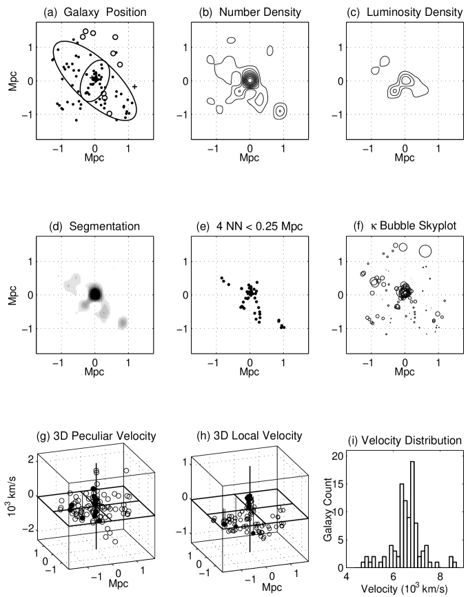
Figure 37: Visualization plots for Abell S301.

Abell S301 (DC-0247-31) is one of the nearest clusters in the study with an estimated distance of $d_{p}(t_{e})=65h^{-1}$ Mpc ($c\overline{z}=6669$ km/s). The surface plots in Figures 37(a)-(e) show the central regions to contain a compact high density core and a smaller second component to the southeast. Comparison of the luminosity and number densities in the central region shows them with similar structure (Figures 37(b) and (c)). In addition, one other subgrouping having density greater than $40\,\mathrm{gal}/(h^{-1}\,\mathrm{Mpc})^{2}$ appears to the southwest, approximately 1.2 $h^{-1}$ Mpc from the centre, and a lower density grouping appears to the northeast at approximately $1.0h^{-1}\,\mathrm{Mpc}$.

Biased by the southeast component, the ellipticity at a mean radius of 0.5 Mpc is $\epsilon=0.36$ at a position angle of $PA=161^{\circ}$. As the mean radius increases, the southwestern and northeastern groupings influence the calculation to shift the position angle with, for example, $\epsilon=0.61$ and $PA=48^{\circ}$ at a mean radius of 1.0 Mpc (Table 2). The variation in position angle is problematic in achieving an elliptical core fit accurate at all radii, but using the average ellipticity parameters from the 0.75-1.0 Mpc mean radii is somewhat better than using a circular fit and yields core parameters of $R_{c}=0.24\,h^{-1}$ Mpc and $\sigma_{0}=133\,\mathrm{gal}/(h^{-1}\,Mpc)^{2}$.

Inspection of Figure 37(i) reveals a distribution with most of the galaxies broadly distributed between $\sim 6300-7000\,\mathrm{km/s}$ and with relatively small tails resulting in a kurtosis of $K=1.9=2.0\sigma_{K}$. The $\chi_{vel}^{2}$ test rejects this as a gaussian distribution at the 99.9% CL. Two of the slowest galaxies ($cz\approx 5000\,\mathrm{km/s}$) are relatively bright compared to the other cluster members and are possibly in the foreground.

While the $\alpha$ test gives no indication for substructure ($P_{\alpha}=24.2\%$), both the $\beta$ and $\kappa$ tests yield statistically significant signals ($P_{\beta}=2\%$ and $P_{\kappa}=0.4\%$). Inspection of the bubble and local velocity plots (Figures 37(f) and (h)) reveals a subcluster in the main component of the core not evident in the surface plots. In particular, Figure 37(h) shows that the local velocities of these galaxies are significantly faster compared to the cluster mean velocity. Overall, the core galaxies have an average velocity of 6968 km/s compared to the mean value for the cluster of 6594 km/s, but 13 galaxies in the core have local velocities exceeding 7200 km/s. These galaxies reside in a very close group near the centre of the main component ($x=-0.10\;\mathrm{to}\;0.10\,h^{-1}\,\mathrm{Mpc}$, $y=-0.02\;\mathrm{to}\;0.11\,h^{-1}\,\mathrm{Mpc}$). The northeastern grouping also appears in the bubble skyplot, but the farthest southwestern grouping is virtually absent. Assessing whether the central velocity structure is truly in the core or is a result of projection effects is required to further determine this cluster’s dynamical configuration and state.

This cluster has been investigated previously for substructure several times, but with significantly fewer redshifts than the 95 used here. Using 26 redshifts, Dressler & Shectman (1988) found no substructure ($P_{\Delta}$ = 34.5%). Using 29 redshifts, Escalera et al. (1994) found no substructure from applying the $\Delta$ and Lee tests ($P_{\Delta}$ = 52.2% and $P_{Lee}$ = 80.0%). Stein (1997) performed the $\Delta$, Lee, and velocity normality tests using 25 members and found no substructure ($P_{\Delta}$ = 29%, $P_{Lee}$ = 63%, and $P_{Norm}$ = 43%). Salvador-Solé, Sanromà, & González-Casado (1993) and Salvador-Solé, González-Casado, & Solanes (1993) using autocorrelation techniques found signs of substructure. Using a KMM method, Kriessler & Beers (1997) found the central region to be bimodal ($P$ = $<$ 0.1%) with the same mode centre locations identified here.

4.20 Abell S333

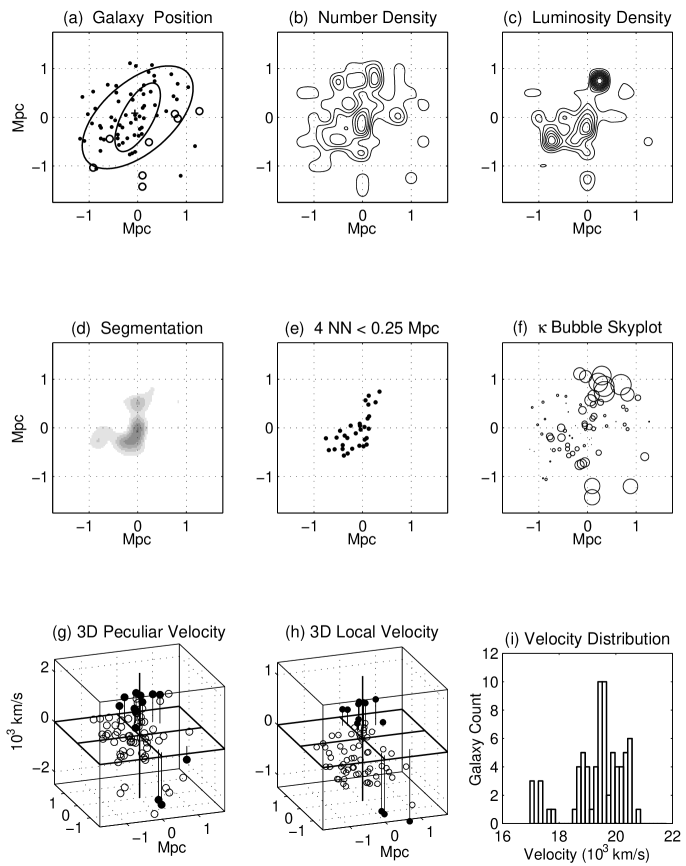
Figure 38: Visualization plots for Abell S333.

Abell S333 is one of the most diffuse clusters in the sample with a low surface density core region (see Figures 38(a) and 38(b)). The luminosity-weighted contour plot (Figure 38(c)) shows the brightest area in the cluster to be separated from the core by approximately 1.0 $h^{-1}$Mpc (projected) northwest of the centre. The high luminosity is due to the brightest galaxy in the cluster ($b_{J}$ = 15.4), but with its velocity being several hundred km/s faster than the cluster mean, it seems unlikely this galaxy is in the foreground.

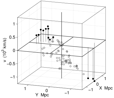
Figure 14: 3D Local Velocity Plot for Abell S333. This is Figure 38(h) rotated counter-clockwise 50^∘ about the z-axis. This view clearly shows the spatial asymmetry in the local velocity with the northern half of the cluster (the leftmost two quadrants in the figure) moving away from the line of sight and with the southern half (the rightmost two quadrants) moving toward the line of sight.

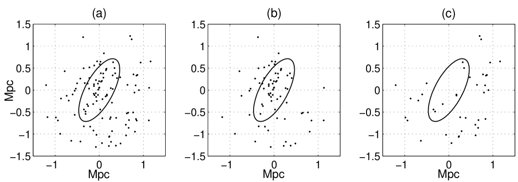
Figure 15: Galaxy positions for Abell S1043 showing the locations of (a) all galaxies, (b) galaxies with $\mathrm{v}<11,000\,\mathrm{km/s}$, and (c) galaxies with $\mathrm{v}>11,000\,\mathrm{km/s}$.

The cluster shows consistent ellipticities and position angles at all radii tested (see Table 2). The ellipticity ranges from $\epsilon$ = 0.59 - 0.41, and the position angle range of $PA$ = $131^{\circ}$ – $156^{\circ}$ is consistently aligned with the high luminosity region (Figures 38(a) and (c)). Given the consistent $\epsilon$ and PA at all distances from the centre, we use the average values ($\epsilon$ = 0.5 and $PA$ = 135^∘) to calculate the core parameters. The resulting values are $R_{c}=0.35\pm 0.01$ and $\sigma_{0}=62\pm 2$.

Inspection of the velocity distribution in Figure 38(i) shows a group of relatively slow galaxies in addition to the unusually-distributed main group. The slow group consists of eight galaxies that have velocities grouped near 17,500 km/s compared to the cluster mean of 19,372 km/s with their positions being indicated by the ‘$\circ$’ symbol in Figure 38(a). Although moving significantly slower than the cluster mean velocity, these galaxies are not obvious foreground contamination: six have magnitudes greater than the cluster mean of 18.1. Two of the galaxies are both brighter than average ($b_{J}$ = 16.9 and 17.8) and significantly slower than average (v = 17,361 and 17,277 km/s). While these two galaxies are possible non-members, their local motions are consistent with neighboring galaxies that are members (see below).

The histogram of the velocities of the majority of the cluster members shows them to be unusually distributed about a narrow peak near the mean velocity. This is reflected by skewness and kurtosis values that are $2.5\sigma$ and $0.9\sigma$ away from normal values, respectively (see Table 4). The $\chi^{2}_{vel}$ velocity test rejects the normal hypothesis with a 99.9% CL. If the eight slowest galaxies are removed from the computation, the $S$ and $K$ statistics move closer to normal; however, the $\chi^{2}_{vel}$ velocity test still rejects the normal hyposthesis at a 93% CL.

The 3D plots and tests show signs of substructure with the $\kappa$ test having the strongest indication with a probability of random occcurence of $P_{\kappa}<0.1\%$ (Table 6). The substructure detected by the $\kappa$ test is found in the high luminosity region to the northwest of the core as seen in the $\kappa$ bubble skyplot (Figure 38(f)). The 3D plots also highlight this area (Figures 38(g) and (h)) where ten galaxies in the northwest quadrant show local velocities above the 95% level of the K-S statistic (represented by the filled circles). The spatial asymmetry of the local velocity plot is seen more clearly when Figure 38(h) is rotated counter-clockwise 50^∘ about the z-axis as shown in Figure 14.

To summarize, Abell S333 has a consistently elongated shape with two relatively luminous regions (the core and the region to the northwest). The luminous region outside the core is also where most of the velocity substructure is found. Together with the (approximate) north-south asymmetry in the local velocity, the cluster shows evidence for dynamics possibly involving rotation, shear, or infall within its supercluster environment.

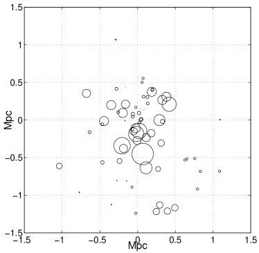
Figure 16: Abell S1043 $\kappa$ bubble skyplot with v $>$ 11,000 km/s members removed.

4.21 Abell S1043

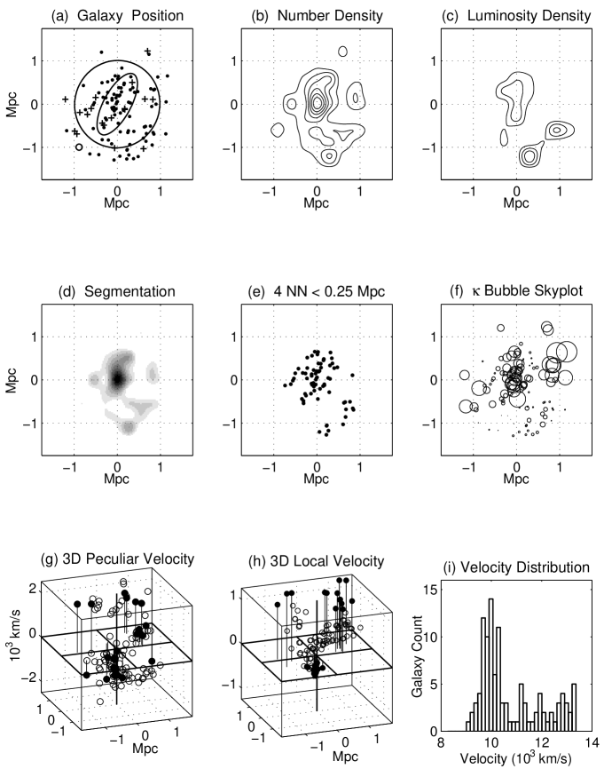
Figure 39: Visualization plots for Abell S1043.

Inspection of the scatter and number density contour plots of Abell S1043 shows a cluster with a well-defined, relatively dense, elongated central region (Figures 39 (a) and (b)). A large number of galaxies at distances greater than $1.0\;h^{-1}$ Mpc from the centroid are located to the south and southwest of the cluster central regions. As most galaxies to the north are less than 0.5 $h^{-1}$ Mpc from the east-west centre line, this gives the cluster an appearance of asymmetry. The luminosity contour plot (Figure 39 (c)) shows two areas outside the core with luminosity the same or greater than the core. The two areas of greatest luminosity appear in the galaxies to the south and southwest mentioned above where the four brightest galaxies are located, but with velocities showing no evidence for obvious non-membership.

At mean radii of 0.5 to 0.75 $h^{-1}$ Mpc, the ellipticity ranges from $\epsilon=0.60$ to $0.43$. with a position angle from $PA=152^{\circ}$ to $169^{\circ}$ (Table 2). At a radius of 1.0 $h^{-1}$ Mpc, the galaxies to the east and west of the core tend to reduce the ellipticity ($\epsilon=0.03$) with no shift to the position angle ($PA=162^{\circ}$). When the mean radius is increased to 1.25 $h^{-1}$ Mpc, the galaxies to the south and southwest influence the calculations such that the ellipticity increases to $\epsilon=0.32$ and the position angle shifts to $PA=16^{\circ}$. To fit the central regions as accurately as possible, the ellipticity and position angles for the $0.5\;\mathrm{and}\;0.75\;h^{-1}\,\mathrm{Mpc}$ dispersion ellipses are used to find a core radius of $R_{c}=0.31\pm 0.01$ and a maximum density of $\sigma_{0}=107\pm 3$.

From Figure 39(i), the velocity distribution is highly skewed (the value of $S=0.86$ is $2.3\sigma$ away from the expected value of zero) with a “slow” group of galaxies between 9,000 and 11,000 km/s having a normal-shaped distribution, and with an almost uniform distribution of “fast” galaxies from 11,000 to 13,500 km/s. For the entire distribution, the $\chi_{vel}^{2}$ test rejects the normal hypothesis with a CL $>$ 99.9%. However, when the fast galaxies are removed, the remaining galaxies have a velocity distribution indistinguishable from a gaussian (CL = 29% to reject). Further analysis reveals that relatively few members of this fast group are located within the 0.5 $h^{-1}$ Mpc mean radius ellipse (see Figure 15).

The two-dimensional plots and tests are dominated by the galaxies to the south and southwest as shown by the segmentation plot (Figure 39(d)), the nearest neighbor plot (Figure 39(e)), and the $\beta$ test result of $P_{\beta}=0.7\%$. Comparison of Figure 15 with Figures 39(b), (d), and (e) show that ten of the faster galaxies are located nearly due west of the central regions, but have only marginal density or connectedness relative to the other concentrations.

Before partitioning the galaxies into the two velocity groups, the 3D tests plots indicate a marginal to high level of substructure: $P_{\alpha}=10.2\%$ and $P_{\kappa}<0.1\%$ (Table 6). However, when the fast group of galaxies mentioned above is removed, the significance is substantially reduced to $P_{\kappa}^{slow}=8.9\%$. Comparison of the $\kappa$ bubble skyplot for the slower group in Figure 16 with Figures 39(f), (g), and (h) reveals that it is the fast galaxies to the west that heavily influence the $\kappa$ test results for all the galaxies. However, even with the fast galaxies removed, the central regions still show indications of substructure dynamics. In particular, there appears to be a possible subcluster near the core that is the source of the relatively large remaining $\kappa$ bubbles in Figure 16.

It is interesting to note that the dispersed galaxies to the south and southwest are not inconsistent with post-merger asymmetries found in the simulations of Pinkney et al. (1996). However other explanations are possible, and a more detailed analysis of the cluster is required.

4.22 APM 917

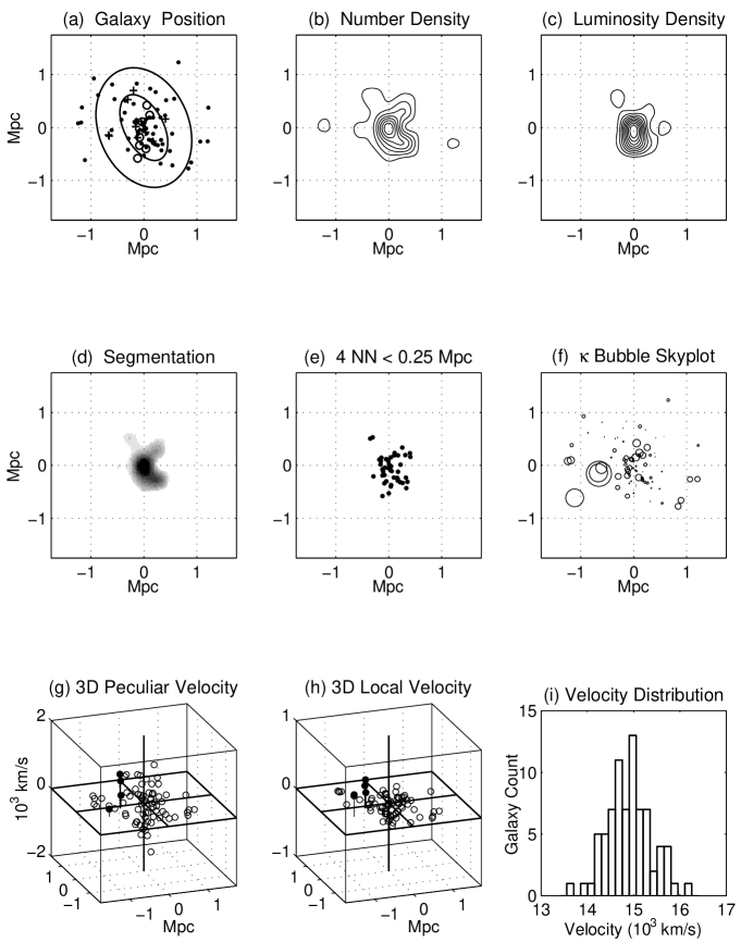
Figure 40: Visualization plots for APM 917.

APM 917 appears to have a high-density, well-defined core (Figures 40(a) – (e)), and does not appear to have regions of high-density galaxy groupings outside the central region with the luminosity being strongly concentrated in the central region (see Figure 40(c)). The velocity distribution appears normal. This appearance of normality is further supported by the skewness and kurtosis statistics ($S=0.18$ and $K=0.03$) as well as the $\chi_{vel}^{2}$ test yielding only a 73% CL to reject the normal hypothesis (see Table 4).

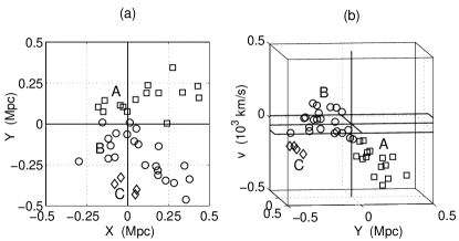
Figure 17: The central region of APM 917 in 2D and 3D Space. Plot (a) shows the central region in 2D space while plot (b) shows the central region in 3D as viewed from the west, using local velocities for the $z$ direction. Members of component A are denoted by squares, component B by circles, and component C by diamonds.

The central region, while well-defined, has an unusual triangular or almost crescent shape. It has a relatively moderate level of ellipticity (Table 2) at all mean radii with varying position angles ($\epsilon$ = 0.45 - 0.27 and $PA=17^{\circ}$ – $56^{\circ}$ for $R$ = 0.5 - 1.25 $h^{-1}$ Mpc). The average of the ellipticity and position angles for the 0.75 and 1.0 $h^{-1}$ Mpc mean radii are used to calculate the King profile core radius and maximum density (Table 3). The cluster core radius at $R_{c}=0.14\pm 0.01$ $h^{-1}$ Mpc is the smallest in the sample and the maximum density, $\sigma_{0}=270\pm 1$, is second highest.

The results of the $\kappa$ test suggest a possibility of substructure with $P_{\kappa}=9.0\%$ (Table 6). Inspection of the $\kappa$ bubble skyplot in Figure 40(f) shows four members to the east of the centre with a high level of $\kappa$ with some lower $\kappa$ values in the central region. The $\alpha$ test indicates a high probability of substructure with $P_{\alpha}$ = 0.6%. Since the $\alpha$ test measures the velocity dispersion-weighted centroid shift when the cluster velocities are randomly shuffled, and there are no obvious subgroupings in the surface distribution, it is expected that the results of this test are due to the presence of significant velocity substructure in the core. A more detailed examination of the central region in the 3D surface-velocity space supports this conjecture.

The central region appears to be composed of three components as seen in Figures 17(a) and (b). We classify galaxies into one of the three components (A, B, or C) based on their 3D proximity to the component. A certain amount of arbitrary judgment is used, and the component boundaries are not meant to be necessarily absolute. When viewed from the west, it is clear that the A and C components are moving slower than the central component, B. All three components have a rather small dispersion among themselves. A random reshuffling of member velocities would result in higher dispersions resulting in lower weights for the component members and, in turn, a higher centroid shift in the $\alpha$ test.

4.23 APM 933

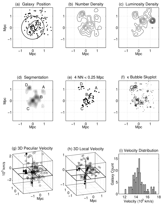
Figure 41: Visualization plots for APM 933.

Inspection of APM 933 galaxy position and number density contour plots, Figures 41(a) and (b), shows a high-density, somewhat elongated core, the centre of which is offset from the cluster mean centroid by $\approx 0.1\,h^{-1}\,\mathrm{Mpc}$. A grouping of galaxies with a density greater than $40\,\mathrm{galaxies}/(h^{-1}\,\mathrm{Mpc})^{2}$ is located approximately $1.3\,h^{-1}\,\mathrm{Mpc}$ to the north-northeast of the centre. This grouping is also readily apparent in the segmentation and nearest neighbors plots, Figures 41(d) and (e). Comparison of the number density and luminosity density contour plots, Figures 41(b)and (c), shows that the light and mass do not exactly overlap for this cluster. Including the grouping to the northeast mentioned above, there are three areas to the north with luminosities equaling or exceeding that of the cluster central region. However, correlation of the velocity-magnitude plot with these high luminosity regions reveals no obvious foreground candidates. In fact, the brightest galaxy in this cluster catalogue (at the position farthest west in Figure 41(c)) has a measured velocity of more than $1.0\sigma$ faster than the cluster mean indicating that it is either an exceptionally bright background galaxy or possesses unusual dynamics.

In general, the ellipticity algorithm converges around moderate to low ellipticity solutions. The elongated appearance of the core is quantified by the ellipticity computation for the $0.5$ and $0.75\,h^{-1}\,\mathrm{Mpc}$ mean radius ellipses yielding yielding values of $\epsilon=0.53$ – $0.40$. The fitted core parameters are $R_{c}=0.36\pm 0.01$ and $\sigma_{0}=91\pm 2$.

From Figure 41(i), the velocity distribution contains a peak at $\approx 14,600\,\mathrm{km/s}$ and an extended tail of galaxies with velocities greater than 16,000 km/s. These two features result in skewness and kurtosis values of $S=0.77$ and $K=0.81$ that are $2.2\sigma_{S}$ and $0.9\sigma_{K}$, respectively, away from the values expected for a normal distribution. The skewness and kurtosis combine such that the $\chi_{vel}^{2}$ test rejects the normal hypothesis with a CL of 97%.

With a value of $P_{\beta}<0.1\%$, the $\beta$ test indicates a high probability for nonrandom asymmetry. Although the $\alpha$ test does not indicate a high probability for nonrandom substructure ($P_{\alpha}=18.5\%$), both the $\kappa$ test ($P_{\kappa}=2.6\%$) and the local velocity plot (Figure 41(h)) reveal several potentially interesting subgroupings and possible bound subclusters labeled A through D in Figure 41(e). The 3D plots again show at least eight of the galaxies in the grouping to the north-northeast identified as D probably reside in a bound subcluster (Figures 41(f)–(h)). In the 3D local velocity plot, seven of the galaxies in this subcluster have a $\leq$ 5% or less probability that the velocity distribution of their nearest neighbors belong to the cluster velocity distribution. The $\kappa$ bubble skyplot and the local velocity plot also show substructure in the central regions highlighted by grouping B that is suggestive of two or three subclusters having motions consistent with merger dynamics or infall, but a more detailed analysis is required for unambiguous identification. A smaller group of six galaxies is found outside the central regions, and is denoted in the nearest neigbors plot as C. Four of these galaxies have velocities within a narrow range of 500 km/s, and likely comprise a small subcluster while the other two galaxies probably do not belong to this grouping. Grouping A does not appear to be a dynamically significant subcluster, and may be a binary with one or two additional galaxies seen in projection in the 2D plots.

4.24 EDCC 365

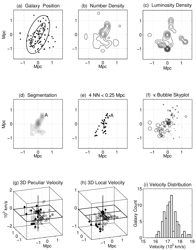
Figure 42: Visualization plots for EDCC 365.

Inspection of EDCC 365 scatter, isodensity, segmentation, and nearest neighbor plots (Figures 42(a), (b), (d), and (e)) shows a relatively diffuse cluster with a well-defined core, a large clump of galaxies just northwest of the core (A), and some structure south and southeast of the core that does not appear to be subclustering. The luminosity contour plot, Figure 42(c), highlights the luminosity of the core although the dominant luminosity signal is in the south due to the presence of the brightest cluster galaxy ($b_{J}=15.1$). The velocity of the brightest galaxy is consistent with cluster membership ($cz=17,868\,\mathrm{km/s}$ compared to the cluster mean redshift of $c\overline{z}=17,773\,\mathrm{km/s}$). The approximate north-south alignment of the groupings biases the ellipticity algorithm to yield relatively high ellipticities of $\epsilon\sim 0.5-0.7$ at position angles $PA\sim 150-160^{\circ}$ (see Table 2). We compute the core parameters by averaging the ellipticities and position angles from the 0.5 and 0.75 $h^{-1}$ Mpc results to find a core radius and maximum density of $R_{c}=0.37\pm 0.01\,h^{-1}$ Mpc and $\sigma_{0}=70\pm 2$.

The velocity histogram (Figure 42(i)) appears normal. The skew and kurtotsis do show some signs of anormality ($S=0.72$ and $K=1.00$) however, the $\chi^{2}_{vel}$ test has only a 83% confidence level to reject the normal hypothesis.

The cluster asymmetry measured by the $\beta$ test yields a marginally significant $P_{\beta}=4\%$ probability of random occurrence, while the $\alpha$ test gives no indication of substructure ($P_{\alpha}=39.1\%$). However, with $P_{\kappa}=0.2\%$, the $\kappa$ test indicates the presence of substructure at a high significance level. From the bubble plot of Figure 42(f), the substructure appears in two distinct regions corresponding to the core and the galaxies to the southeast. These galaxies are also readily apparent in the peculiar and local velocity plots in Figures 42(g) and (h), but do not form a well-defined clump. Correlation of the galaxies in the core with the larger bubbles and the x-y-local velocity plot reveals no obvious subclustering in this region. The velocities of the galaxies in grouping A are consistent with this grouping being a subcluster.

4.25 EDCC 442

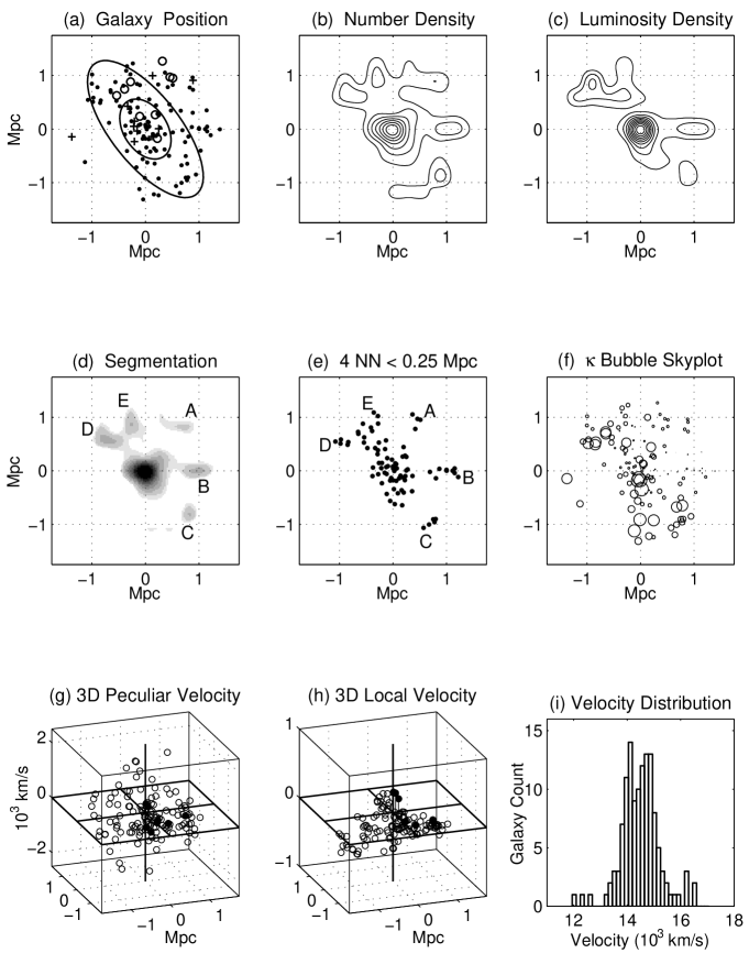
Figure 43: Visualization plots for EDCC 442.

From Figures 43(a)-(e), EDCC 442 is an elongated cluster possessing a relatively dense core. Outside the central regions, there are five groupings with number densities greater than $40\;\mathrm{gal}/(h^{-1}\,\mathrm{Mpc})^{2}$ (labelled in Figure 43(d)). Comparison of Figures 43(b) and (c) shows that the cluster centre of luminosity is closely correlated with the mean arithmetic centre due to the presence of several of the brightest galaxies apparently residing near or at the bottom of the cluster potential well.

The ellipticity computation yields higher ellipticities at the larger mean radii due to the influence of the subgroupings, and smaller ellipticities in the central region, e.g., $\epsilon=0.34$ at $R=0.5\,h^{-1}\,\mathrm{Mpc}$ while $\epsilon=0.58$ at $R=1.0\,h^{-1}\,\mathrm{Mpc}$. Note, however, that the position angle of the core galaxies is aligned with the subgrouping-influenced global cluster position angle of $PA\approx 35^{\circ}$. Using the average ellipticities and position angles for the $0.5\;\mathrm{and}\;0.75\,h^{-1}\,\mathrm{Mpc}$ dispersion ellipses to compute the core parameters of $R_{c}=0.33\,h^{-1}\,\mathrm{Mpc}$ and $\sigma_{0}=113\pm 4\;\mathrm{gal}/(h^{-1}\,\mathrm{Mpc})^{2}$ yields a significantly better fit to the cluster density profile.

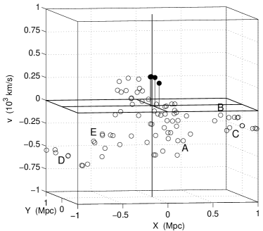
Figure 18: EDCC442 local velocities of the nearest neighbors shown in Figure 43(e). Groupings B, C, D, and E are possible subclusters, and there is velocity structure in the core region.

The velocity distribution as shown in Figure 43(i) is symmetric ($S=<0.01$) but somewhat flattened compared to a normal distribution ($K=1.7=2.1\sigma_{K}$) with a slight indication of bimodality. Nevertheless, the $\chi_{vel}^{2}$ test does not reject this distribution as normal (CL to reject the normal hypothesis = 51%). The three slowest galaxies with $v<12,500\,\mathrm{km/s}$ are probably in the foreground.

Consistent with the appearance of the 2D visualization plots, the $\beta$ test yields a statistically significant asymmetry of $P_{\beta}=3\%$ probability of random occurrence. The two-dimensional substructure reflects apparently real three-dimensional substructure in at least four of the subgroupings noted in Figure 43(d). The nearest neighbor local velocity plot in Figure 18 clearly shows that the galaxies in subgroupings B, C, D, and E have local velocities consistent with their being members of bound subclusters.

The kinematically-weighted centroid shifts tested by the $\alpha$ algorithm do not indicate significant substructure ($P_{\alpha}=24.9\%$). However, with $P_{\kappa}=3.5\%$, the $\kappa$ test does indicate the probable presence of dynamically significant substructure. Correlating the bubble plot of Figure 43(f) with the segmentation/nearest neighbor plots of Figures 43(d)-(e) indicates again that the galaxies in groupings C and D are probable subclusters, and with the transition between D and E being gradual rather than sharp. Consistent with the “stringy” appearance of the local velocities of the nearest neighbors in Figure 18, the bubble plot also gives some indication of core kinematics that may indicate non-virialized core dynamics. The lack of relatively large bubbles at the locations of groupings A, B, and E requires further investigation to distinguish whether these are bound subclusters with velocity distributions indistinguishable from the global distribution, the local grouping motion is transverse to the line-of-sight, or the groupings are only a result of projection effects (as appears likely for grouping A although this grouping does appear to contain a likely bound binary).

5 Summary of Results and Discussion

To begin evaluating the physical significance of the results obtained here, consider that, in principle, any single test can detect the type of substructure to which it is sensitive regardless of the results of any other test. We believe that the methods used here to detect substructure in the galaxy distribution are generally accurate to the confidence levels stated due to the discriminating power of the 3-dimensional tests in substantially reducing (or eliminating) apparent substructure due to projection effects. In particular, the $\kappa$ test results combined with the bubble skyplot and plot of the local velocities/relative positions of the nearest neighbors appears to be a particularly useful combination for identifying true substructure.

However, it should be remembered that it has been demonstrated through Monte Carlo simulation that substructure tests have both “failure to detect” and “false positive” rates (see, e.g., Pinkney et al. 1996). Thus, before summarizing the results of the statistical tests applied to the present sample, it is appropriate to review estimates for the numerical reliability of the $\alpha$ and $\beta$ tests.

Pinkney et al. found that the $\alpha$ test is generally a robust diagnostic of substructure, sensitive to dispersed subclusters, and that its effectiveness is not always diminished by a superposition of the core and a subcluster. In that study, the test identified substructure in 24 out of 36 cases of simulated mergers at a 10% probability of random occurrence, second only to the $\Delta$ test. At a 5% probability level the test detected 16 out of 36 subclusters, and at 1%, 12 out of 36. On the other hand, the test is also found to have relatively high false positive rates at the 10% and 5% significance levels. For example, in a cluster with 100 members, the test incorrectly detected substructure in 23 out of 100 cases at a 10% confidence level. At a 1% confidence level, however, its false positive rate was closer to the other estimators tested (Pinkney et al. 1996).

For the $\beta$ test, the Pinkney et al. study found it to be the second best two-dimensional test out of the four two-dimensional tests that were evaluated; their most robust 2-dimensional test was the Fourier elongation test that was essentially replaced in this study by the ellipticity algorithm. In that work, The $\beta$ test identified substructure in 16 out of 36 cases with a 10% probability of random occurence, 15 cases with a 5% probability, and nine cases with a 1% chance. The false positive rate was found to be 12%, 9%, and 4% for significance levels of 10%, 5%, and 1% using a sample cluster size of 100 galaxies. Thus, it appears the test has a low detection rate and a high false positive rate. This was true for most of the one-dimensional and two-dimensional tests evaluated. As one would expect, the $\beta$ test was effective for detecting deviations from mirror symmetry, but not necessarily circular symmetry. In terms of merger scenarios, the test works best at early stages of merger viewed at right angles but not as well at later stages viewed nearly straight on. Perhaps most importantly, and not explicitly discussed in previous work, is the sensitivity of the results to the choice of cluster centroid.

Given the above comments, it is obviously not possible to make an absolute statement regarding the confidence level at which a particular test yields a true result. In many cases, a final judgment can be rendered by incorporating high-resolution, long-exposure X-ray data. In other cases, there may be no absolute determination possible. However, we believe that the approach used here to combine visualization plots with statistical tests and then to identify sources of positive signatures is robust in mitigating the relatively small probabilities for the statistical tests to yield a false positive or negative recognition.

Table 6: Summary of statistical tests for substructure. The number in the table is the percent probability that the test statistic is the result of a random occurrence.

	Probability in %
Cluster	$\alpha$	$\beta$	$\kappa$	$\chi^{2}_{vel}$
Abell 930	3.0	30.3	5.8	$<0.1$
Abell 957	32.1	0.5	14.4	51.5
Abell 1139	$<0.1$	14.8	$<0.1$	23.6
Abell 1238	6.7	49.7	8.0	86.4
Abell 1620	26.8	0.1	0.9	2.8
Abell 1663	28.9	3.9	0.1	64.4
Abell 1750	1.9	$<0.1$	2.6	1.8
Abell 2734	44.8	0.4	35.3	14.9
Abell 2814	1.3	8.0	6.5	32.0
Abell 3027	44.0	18.8	0.2	0.1
Abell 3094	47.7	9.9	$<0.1$	7.3
Abell 3880	15.9	7.0	22.0	64.3
Abell 4012	1.0	25.9	20.9	4.0
Abell 4013	26.5	1.8	4.3	$<0.1$
Abell 4038	$<0.1$	$<0.1$	$<0.1$	4.1
Abell S141	34.6	23.1	19.8	2.0
Abell S258	36.7	6.6	$<0.1$	29.8
Abell S301	24.2	1.8	0.4	0.1
Abell S333	29.7	24.0	$<0.1$	$<0.1$
Abell S1043	10.2	0.7	$<0.1$	$<0.1$
APM 268	2.8	$<0.1$	2.6	2.2
APM 917	0.6	38.0	9.0	27.0
APM 933	18.5	$<0.1$	2.6	3.3
EDCC 365	39.1	4.1	0.2	17.4
EDCC 442	24.9	2.5	3.5	49.1

The results for the $\alpha$, $\beta$, $\kappa$, and $\chi_{vel}^{2}$ tests are collected in Table 6 where it can be seen that only 4 of the 25 clusters failed to yield at least one signal at or below a 1% probability for random occurrence (or, equivalently, at or greater than a 99% CL where the results have been rounded to the nearest percentile). Table 7 tabulates the results in terms of the number of clusters that yielded substructure at less than the 10%, 5%, and 1% probabilities for random occurrence. Multimodal central regions were detected in about half of the sample, and many of these appear consistent with merger scenarios. In general, the luminosity density in these clusters correlates closely with the number density, the few exceptions probably being due to the small level of incompleteness leaving out a few bright galaxies. However, this should be more closely examined in a future study.

Table 7: The number of clusters showing a substructure signal at less than or equal to a specified probability that the signal is a random occurrence. The entries include clusters whose Monte Carlo probabilities are rounded to the nearest percentile.

Test	10%	5%	1%
$\alpha$	10	8	5
$\beta$	17	13	8
$\kappa$	20	16	11
$\chi^{2}_{vel}$	14	13	6

It is well known that giant elliptical galaxies in clusters usually reside in a region of high galaxy density, either in the central region or in bound subclusters, and it is believed that galaxy-environment interactions significantly affect galaxy formation and evolution. The absence of clear morphological data for most of the galaxies in this catalogue restricts analysis here to correlating brightness with clumpiness (as provided by the luminosity density contour plots). We find that 16 of the 25 clusters contain probable bound subclusters with luminosity density comparable to that in their cores. Of these, 14 clusters contain one or more subclusters in which the first, second, or third brightest galaxy is found. Especially noteworthy are A957, A1663, and A1750 as clusters having subclusters comparable in size to the cluster core and containing a single extremely bright galaxy. The other 11 clusters are A1238, A1620, A2814, A3027/APM268, A3094, S258, S301, S1043, APM933, and EDCC442.

As mentioned in the Introduction, the clusters selected for this study from the 2dFGRS catalogue were required to have at least 70 members in order to have confidence in the statistical results, and to provide a small enough set to allow analysis of individual clusters. With the catalogue utilized for this study not containing clusters with memberships exceeding $N=154$, this selection criterion then naturally resulted in analysing low richness clusters of galaxies which are structures not as well studied as rich clusters and groups. Assessing the robustness of the approach here, it appears that smaller-sized groups in the 2dFGRS catalogue could reliably be analysed using the same methods. Future work with this particular set of clusters includes incorporating data from the recently published 2PIGG catalogue of clusters (Eke et al., 2004) and comparing against recent N-body simulations of cosmological concordance models. More detailed examinations are also planned of selected clusters by including new X-ray data, applying estimators to characterise cluster dynamics, and using analytical tools such as wavelet analysis or the KMM algorithm to further resolve smaller-scale structure.

To summarize, we have presented a survey-level substructure analysis of 25 low richness clusters of galaxies contained in the 2dFGRS cluster catalogue. Most of the clusters possess features such as multi-component core/central regions, bound subclusters well-removed from the centre, pre- and post-merger indicators, and possible signatures of infall, rotation, or shear dynamics. Thus, we find that substructure in these clusters is the rule rather than the exception indicating that, as conjectured by others and supported by some N-body simulations, low richness clusters relax to structureless equilibrium states on very long dynamical time scales (if at all). The results here also show that while doubling the number of redshifts available per cluster does not drastically alter the velocity statistics found in previous studies, the additional information affords a more comprehensive reconstruction of cluster substructure.

Acknowledgments

This research has made use of the NASA/IPAC Extragalactic Database (NED) which is operated by the Jet Propulsion Laboratory, California Institute of Technology, under contract with the National Aeronautics and Space Administration.

Appendix A Visualization plots for the clusters

This appendix presents the set of visualization plots described in Section 3. For each cluster analyzed, plot (a) shows each galaxy position in $(RA,Dec)$ converted to cartesian $(x,y)$ coordinates with superimposed dispersion ellipses for mean radii of 0.5 and 1.0 $h^{-1}$ Mpc. The projected (2-dimensional) galaxy separations are inferred from the proper distance at photon time of emission, $d_{p}(t_{e})$. Following the usual convention, north is along the positive y-axis and east is along the negative x-axis. The filled circles represent galaxies with velocities within 1.3$\sigma$ of the mean velocity, whereas galaxies slower than 1.3$\sigma$ are represented by a open circle, and galaxies faster than 1.3$\sigma$ are shown with a plus sign. For a normal velocity distribution, approximately 10% of the galaxies should fall in the faster or slower group. Plots (b)-(e) are the 2-dimensional visualization plots described in Section 3.2.

Plot (f) is the $\kappa$ “bubble skyplot” described in Section 3.5 where the size of the circles centered on galaxy positions is proportional to the $\kappa$ statistic for each galaxy. As a complement to the substructure implications provided by the velocity statistics and the $\kappa$ test, visualization of potential substructure correlated with the cluster velocity distribution is accomplished through two additional types of plots: the peculiar velocity of each galaxy, $v_{gal}-\overline{v}_{cl}$, plotted in a 3-dimensional position-velocity format, and the “local” velocity constructed from the average velocity of each galaxy and its nearest neighbors, $v_{local}~{}(=\overline{v}_{NN})-\overline{v}_{cl}$, plotted in the same 3-dimensional position-velocity format. The zero point for the peculiar velocities is the cluster average velocity, whereas the zero point for the local velocity is based on the local velocity of the galaxies residing within one core radius of the cluster centre. For these latter two plots, the position of each galaxy is marked by a filled circle when the $\kappa$ statistic for that galaxy has a $\leq 5\%$ probability of random occurrence and an open circle otherwise (the 5% probability threshold is arbitrary and can be varied to indicate the “strength” of a particular grouping). The vertical lines connecting the position of each filled circle galaxy to the midplane are for visualization purposes only. As seen in the individual cluster analyses, the local velocity plot provides a useful visualization complement to the $\kappa$ statistic and bubble plot. Finally, plot (i) shows the histogram of the velocity distribution using a bin size of 150 km s^-1.

References

- Abell (1958) Abell G.O., 1958, ApJS, 3, 211
- Abell, Corwin, & Olowin (1989) Abell G.O., Corwin H.G., Olowin, R., 1989, ApJS, 70, 1
- Ashman, Bird, & Zepf (1994) Ashman K.M., Bird C.M., & Zepf S.E., 1994, AJ, 108, 2348
- Beers, Geller, & Huchra (1982) Beers T.C., Geller M.J., & Huchra J.P., 1982, ApJ, 257, 23
- Beers et al. (1991) Beers T.C. et al., 1991, AJ, 102, 1581
- Bird (1994) Bird C.M., 1994, AJ, 107, 1637
- Bird & Beers (1993) Bird C.M. & Beers T.C., 1993 AJ, 105, 1596
- Bird, Davis, & Beers (1995) Bird C.M., Davis D.S., & Beers T.C., 1995 AJ, 109, 920
- Biviano et al. (2002) Biviano A. et al., 2002, A&A, 387, 8
- Bliton et al. (1998) Bliton M. et al., 1998, MNRAS, 301, 609
- Burgett (1982) Burgett W.S., 1982, Master’s thesis, Univ. of Oklahoma
- Carter & Metcalfe (1980) Carter D. & Metcalfe N., 1980, MNRAS, 91, 325
- Colless (1998) Colless M., 1998, in Mellier Y., Colombi S., eds., IAP meeting, Wide Field Surveys in Cosmology. Editions Frontières, Gif-sur-Yvette, p.77
- Colless et al. (2001) Colless M. et al., 2001, MNRAS, 328, 1039
- Colless & Dunn (1996) Colless M. & Dunn A.M., 1996, ApJ, 458, 435
- Dalton et al. (1997) Dalton G.B. et al., 1997, MNRAS, 289, 263
- Davis et al. (1995) Davis D.S. et al., 1995, ApJ, 440, 48
- De Propris et al. (2002) De Propris R. et al., 2002, MNRAS, 329, 87
- De Propris et al. (2004) De Propris R. et al., 2004, accepted for publication in MNRAS; eprint arXiv:astro-ph/0402652
- Donnelly et al. (2001) Donnelly R.H. et al., 2001, ApJ, 562, 254
- Dressler (1980) Dressler A., 1980, ApJS, 42, 565
- Dressler & Shectman (1988) Dressler A. & Shectman S.A., 1988, AJ, 95, 985
- Eke et al. (2004) Eke V.R. et al., 2004, MNRAS, 348, 866
- Escalera et al. (1994) Escalera E. et al., 1994, ApJ, 423, 539
- Forman et al. (1981) Forman W. et al., 1981, ApJ, 243, L133
- Geller & Beers (1982) Geller M.J. & Beers T.C., 1982 PASP 94, 421
- Girardi et al. (1997) Girardi M. et al., 1997, ApJ 482, 41
- Jones & Forman (1999) Jones C. & Forman W., 1999, ApJ, 511, 65
- King (1972) King I.R., 1972, ApJ, L123
- Kriessler & Beers (1997) Kriessler J.R. and Beers T.C., 1997, AJ, 80
- Krywult, MacGillivray, & Flin (1999) Krywult J., MacGillivray H.T., and Flin P., 1999, A&A, 351, 883
- Kolokotronis et al. (2001) Kolokotronis V. et al., 2001, MNRAS, 320, 49
- Lémonon, L. et al. (1997) Lémonon L. et al., 1997, A&A, 326, 34
- Lumsden et al. (1992) Lumsden S.L. et al., 1992, MNRAS, 258, 1
- Maddox et al. (1998) Maddox S.J. et al., 1998, in Muller V., Gottlober S.G., Mucket J.P., Wambsganss J., eds., Large Scale Structure: Tracks and Traces, World Scientific, Singapore, 91
- Peebles (1993) Peebles P.J.E., 1993, Principles of Physical Cosmology, Princeton University Press, Princeton, NJ
- Pinkney et al. (1996) Pinkney J. et al., 1996, ApJS, 104, 1
- Press et al. (1992) Press W., Teukolsky S., Vetterling W., & Flannery B., 1992, Numerical Recipes, Cambridge University Press, Cambridge
- Quintana & Ramirez (1989) Quintana H., & Ramirez A., 1989, RMxAA, 19, 103
- Ramirez & Quintana (1990) Ramirez A. & Quintana H., 1990, RMxAA, 21, 69
- Rhee, van Haarlem, & Katgert (1991) Rhee G.F.R.N., van Haarlem M.P., & Katgert P., 1991, A&A 246, 301
- Rosati, Borgani, & Norman (2002) Rosati P., Borgani S., & Norman C., 2002, Ann. Rev. Astron. & Astrophys., 40, 539
- Salvador-Solé, Sanromà, & González-Casado (1993) Salvador-Solé E., Sanromà, & González-Casado G., 1993, ApJ, 402, 398
- Salvador-Solé, González-Casado, & Solanes (1993) Salvador-Solé E., González-Casado G., & Solanes J.M., 1993, ApJ, 410, 1
- Schuecker et al. (2001) Schuecker P. et al., 2001, A&A, 378, 408
- Solanes, Salvador-Solé, & González-Casado (1999) Solanes J.M., Salvador-Solé E., & González-Casado G., 1999, A&A, 343, 733
- Stein (1997) Stein P., 1997, A&A, 317, 670
- Trumpler & Weaver (1952) Trumpler R.J. & Weaver H.F., 1952, Statistical Astronomy, Univ. of California Press, Berkeley
- Vick (2004) Vick M.M., 2004, Ph.D. dissertation, Texas Christian Univ.
- West & Bothun (1990) West M.J. & Bothun G.D., 1990, ApJ, 350, 36
- West, Jones & Forman (1995) West M.J., Jones C., & Forman W., 1995, ApJ, 451, L5
- West, Oemler, & Dekel (1988) West M.J., Oemler A., & Dekel A., 1988, ApJ, 327, 1