Disk Temperature Variations and Effects on the Snow Line in the Presence of Small Protoplanets

Abstract

We revisit the computation of a “snow line” in a passive protoplanetary disk during the stage of planetesimal formation. We examine how shadowing and illumination in the vicinity of a planet affects where in the disk ice can form, making use of our method for calculating radiative transfer on disk perturbations with some improvements on the model. We adopt a model for the unperturbed disk structure that is more consistent with observations and use opacities for reprocessed dust instead of interstellar medium dust. We use the improved disk model to calculate the temperature variation for a range of planet masses and distances and find that planets at the gap-opening threshold can induce temperature variations of up to $\pm 30\%$. Temperature variations this significant may have ramifications for planetary accretion rates and migration rates. We discuss in particular the effect of temperature variations near the sublimation point of water, since the formation of ice can enhance the accretion rate of disk material onto a planet. Shadowing effects can cool the disk enough that ice will form closer to the star than previously expected, effectively moving the snow line inward.

1 Introduction

The concept of a “snow line” was introduced by Hayashi (1981) and refers to the distance from the Sun at which the midplane temperature of the preplanetary solar nebula drops to the sublimation temperature of ice. The presence of ice beyond the snow line, which Hayashi calculated to be at 2.7 AU, ought to enhance planet formation and explains the existence of the gas and ice giants in their present locations. Sasselov & Lecar (2000) revisited this issue, adopting an updated protoplanetary disk model in hydrostatic and radiative equilibrium, with little or no accretion heating (passive disk). They find that the snow line can be as close as $\sim 1$ AU, depending on disk parameters. However, if the temperature of the disk varies with height (e.g., D’Alessio et al., 1998), different parts of the disk will reach the sublimation temperature of water, 170 K, at different radii, so rather than a snow “line” in the disk, there will be a snow “transition.” In this paper, we show that the presence of planets themselves can affect where in the disk the snow transition occurs.

We have previously shown that the presence of a protoplanet can affect the temperature structure in the protoplanetary disk (Jang-Condell & Sasselov, 2003, hereafter Paper I). These temperature variations affect where in the disk ice can form. The goal of this study is to quantify this effect by undertaking a parameter study in which we calculate the temperature structure for a variety of planet masses and distances.

This work is a step toward bridging the gap between simulations of disk-protoplanet interactions and analytical models based on observations of protoplanetary disks. High resolution two- and three dimensional simulations help us to understand the hydrodynamic and tidal interactions between protoplanets and disks (e.g., Kley, 1999; Lubow et al., 1999; Bryden et al., 1999; Kley et al., 2001; Bate et al., 2003). However, a major shortcoming of all these codes is that they assume a very simple equation of state and include no radiative transfer effects. Boss (2001) does consider radiative transfer in the diffusion approximation, but these are simulations of relatively massive disks with high accretion rates and include only compressional and viscous heating, whereas our models concern passive disks in which stellar irradiation is the primary source of heating. Generally speaking, simulated protoplanetary disks are typically vertically isothermal and do not include heating from the central star. While they can probe gravitational and tidal effects of a planet in a disk, they cannot account for effects of shadowing and illumination on the temperature structure as a gap opens in a disk.

Conversely, the analytic disk models self-consistently calculate effects of radiative transfer, which is important because a major source of heating in circumstellar disks is irradiation from the central star (e.g., Calvet et al., 1991; Chiang & Goldreich, 1997; D’Alessio et al., 1998; Dullemond et al., 2001). Analytical models show that disk temperature structure can vary greatly with disk height due to heating at the surface from stellar irradiation and viscous heating at the midplane. However, these models cannot account for perturbations in the disk such as those imposed by the presence of a planet because they only consider radiative transport in one or two dimensions. Monte Carlo simulations of radiative transfer on a disk with a gap created by a planet have been done, but these models are essentially two-dimensional as well (Rice et al., 2003; Whitney et al., 2003). These models are interesting from an observational point of view because large planets are able to significantly change the disk structure, but they do not address what happens to planets below the gap-opening threshold, where planet growth and migration are poorly understood.

The temperature structure of a disk, particularly in the vertical direction, can have an important effect on the dynamics of disk-protoplanet interactions since waves in disks do not necessarily carry energy evenly with height if it is not vertically isothermal (Lubow & Ogilvie, 1998). The local temperature structure can significantly affect how waves are dissipated in the disk, which will in turn affect tidal torques and migration rates.

In this paper, we make a number of modifications to the model presented in Paper I for calculating radiative transfer on perturbed disks, primarily in the calculation of the disk properties. These changes are described in detail in §§2 and 3. The algorithm for calculating radiative transfer remains essentially the same.

In §2, we calculate the structure of the unperturbed disk, in §3 we calculate the effect of a protoplanet on the disk structure, and in §4 we review the method of calculating radiative transfer on a three-dimensional perturbation in the disk. In §5 we apply the revised method and analyze the results. We compare the results with those previously obtained in Paper I, calculate the effect on the temperature of the disk photosphere over varying planet masses and distances, and discuss how these temperature variations change the locations where ice can form in the disk. Section 6 is a discussion of the results and implications.

2 Disk Structure

We assume that the gas and dust in the disk is well-mixed, with the dust primarily responsible for the opacity. The disk is flared, and has a temperature inversion due to radiative heating at the disk surface from the central star.

To calculate the unperturbed disk structure, we adopt the formalism developed by Calvet et al. (1991) and D’Alessio et al. (1998, 1999), with some simplifying assumptions. The parameters we use to describe the disk structure are the density $\rho(r,z)$, temperature $T(r,z)$, and optical depth $\tau(r,z)$. We define $\tau$ without a subscript to be the optical depth of the disk to its own radiation perpendicular to the disk.

We assume that the disk is locally plane parallel to decouple the radial and vertical dependencies of the disk properties. For a given radius $r$, the vertical structure is calculated as follows. The optical depth is given by

$$\tau(z)=\int_{z}^{z_{\infty}}\chi_{R}\rho(z^{\prime})dz^{\prime}.$$ (1)

The density and temperature are calculated assuming hydrostatic equilibrium,

$$\frac{dP}{dz}=-\rho g_{z}$$ (2)

where $P$ is the pressure and $g_{z}$ is the gravitational acceleration perpendicular to the disk. We assume the ideal gas law, $P=\rho kT/\bar{m}$, where $k$ is the Boltzmann constant, $T$ is the temperature, and $\bar{m}$ is the mean molecular weight of the gas, which we assume to be primarily molecular hydrogen.

D’Alessio et al. (1998, 1999) account for turbulent and convective energy transport, as well as radiative transfer in their disk models; however, they find that radiative transfer is the primary mechanism for energy transport, especially in the upper layers of the disk. Indeed, while Calvet et al. (1991) use a simplified set of equations for calculating the disk structure, their results give a close match to D’Alessio et al. (1998). For these reasons, we shall ignore turbulent and convective fluxes and use the simpler set of equations from Calvet et al. (1991).

The temperature in the disk as a function of optical depth and angle of incidence of stellar radiation $\mu_{0}$ can be expressed as

$$T(\tau,\mu_{0})=[T_{v}^{4}(\tau)+T_{r}^{4}(\tau,\mu_{0})]^{1/4}$$ (3)

where $T_{v}$ and $T_{r}$ are temperatures due solely to viscous heating and stellar irradiation, respectively.

We assume that viscous flux is generated at the midplane and transported radiatively in a grey atmosphere so that

$$T_{v}=\left[\frac{3F_{v}}{8\sigma_{B}}(\tau+2/3)\right]^{1/4}$$ (4)

where $\sigma_{B}$ is the Stefan-Boltzmann constant. The viscous flux $F_{v}$ at a distance $r$ for a star of mass $M_{\star}$ and radius $R_{\star}$ accreting at a rate $\dot{M}_{a}$ is

$$F_{v}=\frac{3GM_{\star}\dot{M}_{a}}{4\pi r^{3}}\left[1-\left(\frac{R_{\star}}{r}\right)^{1/2}\right]$$ (5)

(Pringle, 1981).

To get $T_{r}$, we adopt the equations for the flux and mean intensity for the diffuse stellar radiation field ($F_{s}$ and $J_{s}$) and the differential equations for the flux and mean intensity of the disk’s own radiation ($F_{d}$ and $J_{d}$) from D’Alessio et al. (1998). We then solve the differential equations for $F_{d}$ and $J_{d}$ using the boundary condition for relating disk and stellar fluxes, as in Calvet et al. (1991):

$$F_{s}+F_{d}=F_{\mbox{\footnotesize irr}}e^{-\tau_{s}/\mu_{0}}$$ (6)

Solving, we obtain the same equations for the temperature as in Calvet et al. (1991) with $q\equiv\chi_{P}^{\star}/\chi_{R}$, except

$$C_{2}^{\prime} = \frac{(1+C_{1})}{\mu_{0}}\left(\frac{\chi_{P}^{\star}}{\kappa_{P}}-\frac{3\mu_{0}^{2}}{q}\right),$$ (7)

$$C_{3}^{\prime} = C_{2}\beta\left(\frac{\chi_{P}^{\star}}{\kappa_{P}}-\frac{3}{q\beta^{2}}\right).$$ (8)

We use the opacities from D’Alessio et al. (2001) using a dust model with parameters $a_{\mathrm{max}}=1\,\mbox{mm}$ and $p=3.5$. For simplicity, we assume that the dust opacities are constant throughout the disk, even though disk temperatures are typically above the ice sublimation point close to the star and at the surface of the disk, and below the sublimation point farther from the star and near the midplane. To test our assumption of constant opacities, we calculate the our models using the opacities at $T=100$ and 300 K and typically find that the results do not change much.

The upper boundary condition is set so that $P(z_{\infty})=10^{-10}$ dyne, and we integrate the equations for $\tau$, $\rho$, and $T$ down to the midplane using some initial guess for $z_{\infty}$. The other boundary condition is that we match the total integrated surface density

$$\Sigma=\int_{-z_{\infty}}^{z_{\infty}}\rho dz$$ (9)

with the surface density given by a steadily accreting viscous disk

$$\Sigma=\frac{\dot{M}}{3\pi\nu}\left[1-\left(\frac{R_{\star}}{r}\right)^{1/2}\right]$$ (10)

(Pringle, 1981). We adopt a standard Shakura-Sunyaev viscosity with $\nu=\alpha c_{s}H$ (Shakura & Sunyaev, 1973). This boundary condition is required to account for the effect of viscosity on the disk structure, since we do not treat the propagation of turbulent and convective fluxes. This approximation is justified by Fig. 7 in D’Alessio et al. (1998), which shows that the integrated surface density profile of the detailed calculated model closely matches equation (9). Depending on the difference between equation (9) and equation (10), we adjust our guess for $z_{\infty}$ until the values for $\Sigma$ converge.

The angle of incidence, $\mu_{0}$, depends on slope of surface $dz_{s}/dr$, where $z_{s}$ is the “surface” of the disk, where $\tau_{s}/\mu_{0}=2/3$. To get a self-consistent answer for $\mu_{0}$ we iteratively calculate the vertical structure of the disk at intervals of $\Delta\log r=\frac{1}{2}\log 2$, calculating the slope of the surface between intervals of $r$.

For our fiducial disk-star system, we take $M_{\star}=0.5\>\mathrm{M}_{\sun}$, $R_{\star}=2\>R_{\sun}$, $T_{\star}=4000\>K$, $\dot{M}=10^{-8}\>\mathrm{M}_{\sun}\>\mbox{yr}^{-1}$, and $\alpha=0.01$. We calculate the structure of the disk from 0.25 to 4 AU. Figures 1 and 2 summarize the features of this circumstellar disk. In Figure 1, we plot the surface density and mass profile of the disk compared to a typical minimum mass solar nebula (MMSN) with $\Sigma\propto r^{-3/2}$ and enclosed disk mass of $0.01\>\mathrm{M}_{\sun}$ at 50 AU. Beyond 4 AU, we have extrapolated the surface density and mass profiles, assuming a power law. The power-law slope is much shallower for the calculated disk than for the MMSN model, so we expect much more of the disk’s mass to be at larger radii than the MMSN model would predict. The two dust models are differentiated by line type: solid for 300 K, and dashed for 100 K.

Figure 1: Surface density (upper) and mass (lower) profiles of the structure calculated for the fiducial disk model. The solid and dashed lines represent models using opacities for dust at 300 K and 100 K, respectively. Profiles beyond 4 AU are extrapolated. For comparison, the profiles for a disk with $\Sigma\propto r^{-3/2}$, normalized so that the enclosed disk mass at 50 AU is $0.01\>\mathrm{M}_{\sun}$, are plotted as dotted lines.

Figure 2: Temperature and vertical profiles at the indicated heights in the disk. The solid and dashed lines represent the 300 K and 100 K dust models, respectively, in both the upper and lower plots. Upper panel: The temperature profiles are represented by filled triangles for the surface, open squares for the photosphere, open triangles for the midplane, and crosses for the viscous temperature at the photosphere. Lower panel: The values of various disk heights in the disk are represented by filled triangles for the surface, open squares for the photosphere, and open triangles for the thermal scale height.

In Figure 2, we show the temperature profile at various heights in the disk, and the locations of those heights. Again, the solid and dashed lines show results using the 300 K and 100 K dust models, respectively. The surface of the disk is defined to be where most of the stellar radiation is absorbed, i.e., where $\tau_{s}/\mu_{0}=2/3$. We define the photosphere of the disk to be where $\tau=2/3$, and the thermal scale height is $(c_{s}/v_{\phi})r$, where $c_{s}$ is the isothermal sound speed measured at the midplane and $v_{\phi}$ is the Keplerian speed. The upper plot shows temperatures at the surface (filled triangles), the photosphere (open squares), and the midplane (open triangles). We also plot the viscous contribution temperature at to the midplane temperature (crosses). The surface of the disk is always hotter than the photosphere, because the surface gets the most direct heating from stellar irradiation. The photosphere is at many optical depths to the stellar irradiation, both due to the difference in opacities and because of the grazing angle of incidence of stellar radiation to the surface. The midplane temperature is much higher than even the surface temperature at small $r$ because viscous heating dominates close to the star – note that the midplane temperature is nearly equal to the viscous temperature $\lesssim 1$ AU. However, viscous heating falls off more rapidly than irradiation heating with distance, so at larger radii ($\gtrsim 8$ AU), the midplane temperature becomes close to the photosphere temperature. For optical depths $\tau\gtrsim 2/3$, we expect $T_{r}$ to be nearly constant, so in the absence of viscous heating, the midplane and photosphere should be nearly isothermal.

In Figure 3, we show the vertical structure of the disk in optical depth, temperature, and density at a distance of 1 AU. As in Figures 1 and 2, the solid and dashed lines indicate the 300 and 100 K dust models, respectively. The top plot shows the variation of optical depth with height in the disk. The vertical lines indicate the location of the photosphere, where $\tau=2/3$ for the respective dust models. The middle plot shows the temperature structure, which rises toward the midplane as a result of viscous heating, reaches a minimum near the location of the photosphere, and rises again at the disk surface as a result of heating from stellar irradiation. The bottom plot shows the vertical density profile of the disk, and for comparison we have plotted the profile of a vertically isothermal disk at 220 K as a dotted line. The temperature affects the density structure by increasing the density as temperature decreases, and vice versa. The density in our disk model can differ from an isothermal model by an order of magnitude or more due to the variations in temperature, so it is important to accurately and self-consistently solve for the temperature and density profiles.

Overall, the difference between the 100 and 300 K dust models is very small, at the level of a few percent. This justifies our assumption that the opacity is constant throughout the disk, and we assume the dust model of 300 K for the remainder of the paper.

Figure 3: Vertical structure of the fiducial disk at 1 AU. Solid and dashed lines represent 300 K and 100 K dust models, respectively. The vertical lines mark the locations of the photosphere. From top down, the plots show the variation of the optical depth, temperature, and density of the disk vs. disk height. The dotted line shows the density profile of a vertically isothermal disk.

3 Protoplanet-Induced Density Perturbations

We calculate the effect of a protoplanet on the disk in hydrostatic equilibrium in the vertical direction. The unperturbed density and pressure structure, $\rho$ and $P$, satisfy

$$\frac{1}{\rho}\frac{dP}{dz}=-\frac{GM_{\star}z}{r^{3}}.$$ (11)

We express the perturbed density and temperature structure, $\rho^{\prime}$ and $P^{\prime}$, as

$$\frac{1}{\rho^{\prime}}\frac{dP^{\prime}}{dz}=-\frac{GM_{\star}z}{r^{3}}-\frac{Gm_{p}z}{(x^{2}+y^{2}+z^{2})^{3/2}}$$ (12)

Now,

$$\frac{1}{\rho}\frac{dP}{dz}=\frac{kT}{\bar{m}}\left(\frac{d\ln\rho}{dz}+\frac{d\ln T}{dz}\right).$$

In general,

$$\left|\frac{d\ln\rho}{dz}\right|\gg\left|\frac{d\ln T}{dz}\right|$$

so we can write

$$\frac{1}{\rho}\frac{dP}{dz}\approx\frac{kT}{\bar{m}}\frac{d\ln\rho}{dz},\quad\mbox{and}\quad\frac{1}{\rho^{\prime}}\frac{dP^{\prime}}{dz}\approx\frac{kT^{\prime}}{\bar{m}}\frac{d\ln\rho^{\prime}}{dz}.$$ (13)

Calculating the temperature self-consistently is not really feasible, so we set $T^{\prime}\approx T(z_{0})$, the midplane temperature, then equation (12) integrates to

$$\rho^{\prime}=C\rho\exp\left[\frac{1}{c_{s}^{2}}\frac{Gm_{p}}{(x^{2}+y^{2}+z^{2})^{1/2}}\right]$$ (14)

where $c_{s}$ is the midplane isothermal sound speed. For simplicity, we assume that the midplane density is unchanged, so

$$\rho^{\prime}=\rho\exp\left\{\frac{Gm_{p}}{c_{s}^{2}}\left[\frac{1}{(x^{2}+y^{2}+z^{2})^{1/2}}-\frac{1}{(x^{2}+y^{2})^{1/2}}\right]\right\}$$ (15)

If we define the isodensity contour at the density of the unperturbed disk surface to be the perturbed surface, the shape of the perturbation is a depression, as shown in Figure 4. This example is for a 11 $\mathrm{M}_{\earth}$ planet at 1 AU in the fiducial disk, so that the Hill radius is 0.63 of the thermal scale height. When this surface is irradiated at grazing incidence, as from a central star, one side of the well will be shadowed and the other side will experience more direct illumination. The effect on the temperature structure due to radiative heating and cooling is calculated as described in the following section.

Figure 4: The shape of the perturbed surface for a 11 $\mathrm{M}_{\earth}$ planet at 1 AU in the fiducial disk. All units are in AU.

4 Radiative Transfer on Perturbations

To calculate radiative transfer on a perturbation, we use the method outlined in Paper I. We define the surface of the perturbation to be the isodensity contour at the density of the unperturbed surface, and numerically integrate the total contributions to the radiative flux at a given point over this surface using the equation

$$B_{\mathrm{tot}}=\frac{1}{\pi}\int B(\tau_{d},\mu)\,\nu\;\delta\Omega$$ (16)

We refer to the spatial variation of $B_{\mbox{\footnotesize tot}}{}$ as the illumination pattern in the disk. In Figure 5, we illustrate the illumination pattern in the photosphere of the fiducial disk at 1 AU in the vicinity of a planet of mass 11 $\mathrm{M}_{\earth}$. We can easily see the effect of shadowing and illumination in terms of lower or higher values of $B_{\mbox{\footnotesize tot}}{}$.

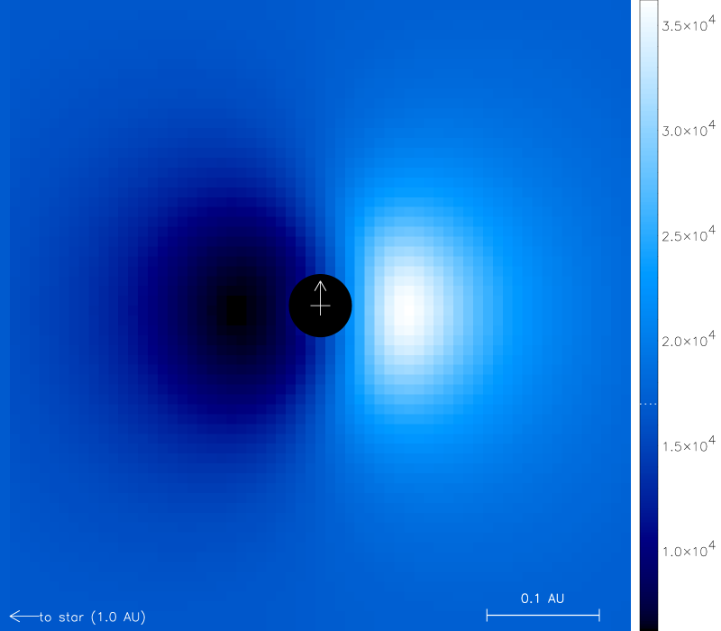
Figure 5: The illumination pattern around a 11 $\mathrm{M}_{\earth}$ planet at 1 AU in the fiducial disk. The black circle shows the extent of the Hill radius, with the white cross indicating the position of the planet. The upward-pointing arrow shows the direction of the motion of the planet. The color bar indicates the scaling of $B_{\mbox{\footnotesize tot}}{}$ in units of energy flux.

To calculate the temperature distribution, we assume that the gas travels on streamlines in Keplerian orbits, which is an adequate assumption outside the Hill radius. The gas heats and cools radiatively according to

$$C\frac{\partial T}{\partial t}=B_{\mbox{\footnotesize tot}}{}-\sigma T^{4}$$ (17)

where $C$ is the specific heat per unit surface area of the disk, defined as $C=k\Sigma/\bar{m}$ where $\Sigma$ is the total surface density. The resulting temperature profile for the disk-planet system shown in Figure 5 is shown in Figure 6.

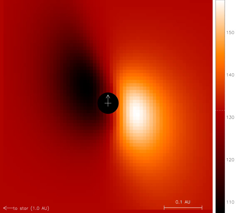
Figure 6: The temperature profile around a 11 $\mathrm{M}_{\earth}$ planet at 1 AU in the fiducial disk. Markings on the plot are the same as Figure 5, except that the color bar here indicates the temperature scale in kelvins.

5 Results

5.1 Comparison of Results with Paper I and Estimate of Model Uncertainties

In §§2 and 3 we discussed the changes we have made to the disk model of Paper I. Although we now directly calculate the disk surface from the isodensity contour instead of approximating its shape, the shape of the perturbation surface changes very little. However, the detailed calculation of disk structure including more realistic opacities for circumstellar disks do have an important effect.

For comparison, we reproduce the temperature profile in the disk photosphere for a 10 $\mathrm{M}_{\earth}$ planet at 1 AU from Paper I in Figure 7. Comparing this to Figure 6, two differences are immediately obvious. The area over which the temperature is perturbed is much larger in Figure 6, particularly in the radial direction. Also, the magnitude of the perturbation is much larger, with temperatures varying from 107 K to 158 K in Figure 6, versus 124 K to 142 K in Figure 7.

Figure 7: Temperature profile of the disk photosphere near a 10 $\mathrm{M}_{\earth}$ planet at 1 AU in orbit around a star of 0.5 M_☉, taken from Paper I, Fig. 7

The new method of calculating disk structure gives a much lower surface density at 1 AU than one would expect from a MMSN disk, which we had previously used to find the surface density, as can be seen from Figure 1. This means a smaller specific heat, which means a faster radiative heating/cooling rate, which means less smearing out of the temperature gradient from differential disk rotation. The shadow and illuminated region cool and heat more effectively; hence, the larger size of the temperature perturbation in the photosphere.

The new opacities adopted in this paper are much are smaller than those used in Paper I, which used opacities representative of interstellar medium dust rather than disk dust. Since the optical depths are smaller, this means that the photosphere is deeper, that is, farther away from the surface. This increases the amount of solid angle that the shadowed or illuminated region subtends in reference to a point in the photosphere. This also helps to increase the area of the temperature perturbations.

The new opacities also give a smaller ratio of opacities, which means that stellar radiation penetrates the disk better, increasing the effect of the irradiation on the temperature structure of the disk. This is the main reason for the increase in the magnitude of the temperature variation over those reported in Paper I, although the previously mentioned effects also have some effect. A comparison of the temperature variations is shown in Figure 8. The temperature variations reported in this paper are $\sim 2.5-3$ times greater than those reported previously. Also, in the previous paper, the magnitude of temperature decrements were consistently greater than temperature decrements. However, this trend is reversed in this paper because $\mu_{0}$ is smaller: $\mu_{0}=0.045$ in Paper I and $\mu_{0}=0.031$ here. The smaller value of $\mu_{0}$ means that the disk gets less direct radiation in the unperturbed state, so that regions that get more direct illumination from the star get relatively hotter.

Figure 8: Comparison of temperature variations between Paper I and results presented here. Fractional temperature variation is plotted vs. planet mass. The lines show temperature maxima and minima for the parameter study presented in this paper, and the crosses show results from Paper I.

In summary, the comparison between the results of Paper I and this paper illustrate the range of model uncertainties involved in calculating radiative transfer in disks. In this paper, we have tried to assume parameters for our model that accurately represent conditions that are observed in real disks; however, those assumptions are subject to change as increased telescope resolution and sensitivity reveal more about disks.

5.2 Results of the Parameter Study

In this section, we present the results of varying the mass and distance of the planet within the same fiducial disk.

The gap-opening threshold is where the Hill radius is the same as the thermal scale height of the disk. For this reason, we parameterize the mass of a planet in terms of $r_{\mathrm{H}}/h$, where $h$ is thermal scale height of the disk. We examine planets at distances of $0.5$, 1, 2, and 4 AU, with $r_{\mathrm{H}}/h$ ranging from $0.25$ to 1. Table 1 summarizes the distances and masses of the planets examined in our parameter study.

Table 1: Planet masses, in $M_{\oplus}$

$r$	$r_{\mathrm{H}}/h$
(AU)	0.25	0.31	0.40	0.50	0.63	0.79	1.00
0.5	0.596	1.19	2.38	4.77	9.53	19.1	38.1
1	0.689	1.38	2.76	5.51	11.0	22.0	44.1
2	0.838	1.68	3.35	6.70	13.4	26.8	53.6
4	1.13	2.26	4.51	9.03	18.1	36.1	72.2

Figure 9 summarizes the variations in temperature produced by changing planet mass and distance. The solid line represents the unperturbed photospheric temperature versus radius. The symbols represent different planet masses, parametrized by the ratio of the Hill radius to the disk scale height. As indicated, planets can induce temperature variations of several tens of K, and still be below the gap-opening threshold. The minimum photospheric temperature at any given radius, i.e., in the absence of radiative heating from the star, is the viscous temperature at $\tau=2/3$, given by $T_{v}=(F_{v}/2\sigma_{B})^{1/4}$. This temperature is indicated by the dotted line. At small distances, the minimum temperatures become limited by viscous heating, since viscous heating contributes more to the photospheric temperature at smaller radii.

Figure 9: Temperature vs. distance. The solid line shows unperturbed temperature, and the dotted line shows the viscous temperature. The symbols below and above the line represent minimum and maximum temperature, respectively, for the indicated planet size.

Figure 10 (left) shows the fractional temperature variation versus planet mass. Each line represents a different distance to the star. The lines above and below $\Delta T/T_{0}=0$ show maximum and minimum temperatures, respectively. The temperature variation can be as much as $\pm 30\%$ for the largest planets studied. If we plot the fractional temperature variation versus $r_{\mathrm{H}}/h$, as in Figure 10 (right), the lines lie almost coincident, indicating that the relevant scale is $r_{\mathrm{H}}/h$, not the planet mass. The divergence of the minimum temperature toward higher $r_{\mathrm{H}}/h$ can be explained by the rise in viscous heating as the distance to the star becomes smaller. Since only stellar irradiation heating is changed by the presence of a planet in our model, viscous heating sets a lower bound to the temperature. The viscous temperature goes as $r^{-3/4}$ while the stellar radiation temperature goes as $r^{-1/2}$, so that close to the star, viscous heating dominates.

Figure 10: Fractional temperature variation vs. planetary size. Left: Horizontal axis is planet mass in $\mathrm{M}_{\earth}$. Right: Horizontal axis is $r_{\mathrm{H}}/h$.

5.3 Hot and Cold Spots and Their Effect on the “Snow Line”

Figures 11 and 12 show the vertical temperature cross sections for a sampling of planet masses and distances. At each sampled distance from the star, two plots are shown: a planet at the gap-opening threshold where $r_{\mathrm{H}}=h$, and a planet that has $r_{\mathrm{H}}=h/2$. In each plot, the planet is located at the origin, with the horizontal axis in the radial direction and the vertical axis indicating height above the midplane. The units are in AU and the star is positioned to the left. Note the cooling due to shadowing to the left of the planet and heating due to illumination on the right. The contours indicate isotherms of 140 K (dotted line), 170 K (solid line) and 200 K (dashed line). The contour corresponding to 170 K is of particular interest, because this is the sublimation temperature of water.

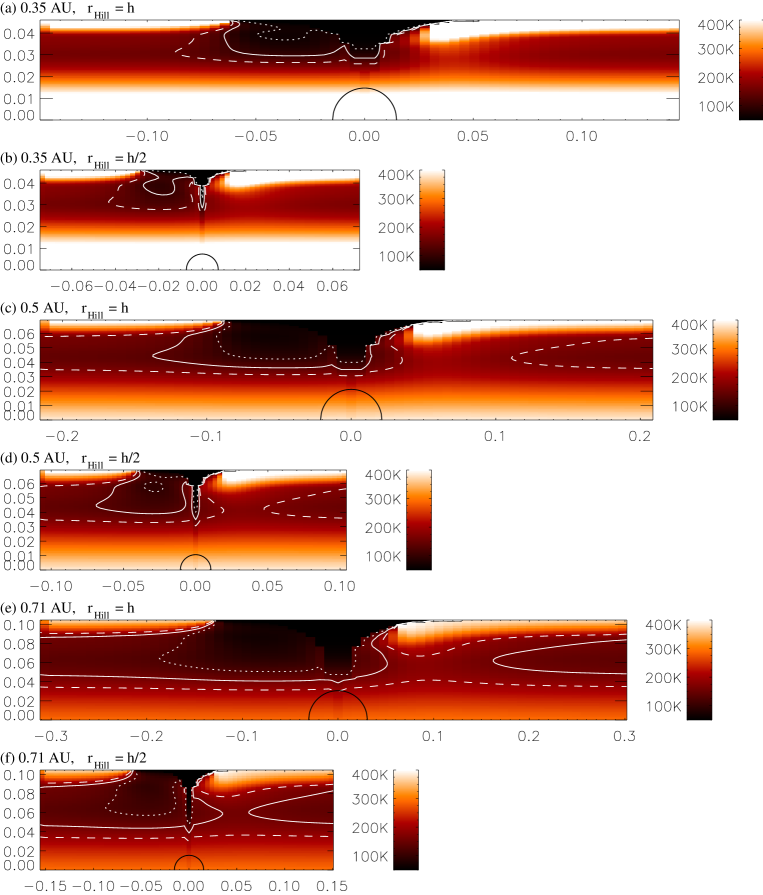
Figure 11: Vertical temperature cross-sections for a selection of planet models. The planet is located at the origin and the star is off to the left. Radiation from the star strikes the surface at grazing incidence. The color bars indicate the temperature scale. The white temperature contours correspond to 140 K (dotted line), 170 K (solid line) and 200 K (dashed line). The black semi-circle centered at the planet’s position indicates the Hill radius. Units on the horizontal and vertical axes are in AU, and indicate distance radially and vertically from the midplane, respectively. (a) $m_{p}=35.9\>\mathrm{M}_{\earth}{}$ ($r_{\mathrm{H}}=h$) at 0.35 AU, (b) $m_{p}=4.49\>\mathrm{M}_{\earth}{}$ ($r_{\mathrm{H}}=h/2$) at 0.35 AU, (c) $m_{p}=38.1\>\mathrm{M}_{\earth}{}$ ($r_{\mathrm{H}}=h$) at 0.5 AU, (d) $m_{p}=4.77\>\mathrm{M}_{\earth}{}$ ($r_{\mathrm{H}}=h/2$) at 0.5 AU, (e) $m_{p}=40.8\>\mathrm{M}_{\earth}{}$ ($r_{\mathrm{H}}=h$) at 0.71 AU, and (f) $m_{p}=5.1\>\mathrm{M}_{\earth}{}$ ($r_{\mathrm{H}}=h/2$) at 0.71 AU.

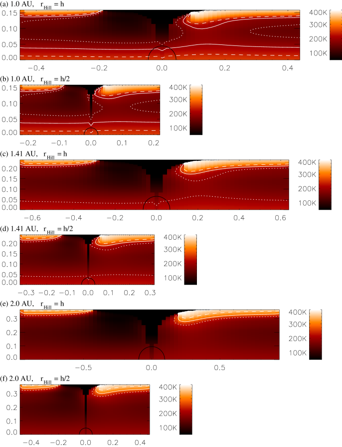
Figure 12: Vertical temperature cross-sections for a selection of planet models. See Figure 11 for details. (a) $m_{p}=44.1\>\mathrm{M}_{\earth}{}$ ($r_{\mathrm{H}}=h$) at 1.0 AU, (b) $m_{p}=5.51\>\mathrm{M}_{\earth}{}$ ($r_{\mathrm{H}}=h/2$) at 1.0 AU, (c) $m_{p}=48.5\>\mathrm{M}_{\earth}{}$ ($r_{\mathrm{H}}=h$) at 1.41 AU, (d) $m_{p}=6.06\>\mathrm{M}_{\earth}{}$ ($r_{\mathrm{H}}=h/2$) at 1.41 AU, (e) $m_{p}=53.6\>\mathrm{M}_{\earth}{}$ ($r_{\mathrm{H}}=h$) at 2.0 AU, and (f) $m_{p}=6.7\>\mathrm{M}_{\earth}{}$ ($r_{\mathrm{H}}=h/2$) at 2.0 AU

.

In this section, we shall define “hot” to be above 170 K, and “cold” to be below 170 K. We define a cold (hot) spot as a region that is colder (hotter) than 170 K in a layer that would be above (below) 170 K in the absence of a planet, and we determine the masses of the hot and cold spots in the disk as a function of planet mass and distance. We find that the correlation between spot mass and planet mass is approximately linear, as shown in Figure 13. The points connected by solid lines show spot mass versus planet mass at the distances indicated, blue lines for cold spots, and red lines for hot spots. The corresponding dotted lines show the linear fits for each of the curves.

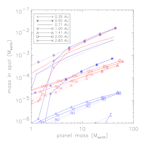
Figure 13: Masses of hot and cold spots vs. planet mass. The symbols represent different distances from the star, as indicated in the legend, red for hot spots and blue for cold spots. The solid lines represent the data points, and dotted lines represent the corresponding linear fits to the data.

We compare the masses of the hot and cold spots to the amount of mass in the planet’s accretion zone, which we will approximate as $4\rho r_{\mathrm{H}}^{3}/3$, the amount of disk material within the planet’s Hill sphere. Then the mass of the accretion zone also scales linearly with planet mass, since $4\rho r_{\mathrm{H}}^{3}/3=m_{p}(4\rho a^{3}/9M_{\star})$, so the ratio of spot mass to the mass of the accretion zone will also be approximately constant. Figure 14 shows how this ratio varies with distance from the star, for both hot and cold spots.

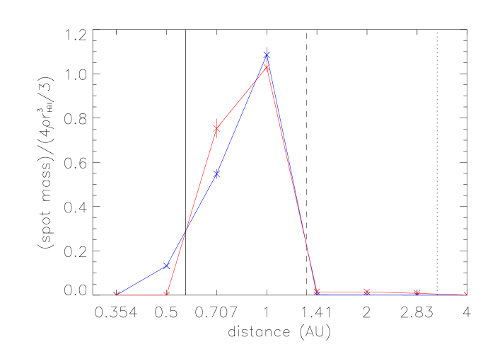
Figure 14: Ratio of spot mass to mass of accretion zone vs. distance. The blue line represents the cold spot mass ratio, and the red line represents the hot spot mass ratio. Errors bars are derived from curve-fitting. The solid vertical line represents the beginning of the snow transition, where the disk begins to drop below 170 K. The dashed (dotted) line shows where the midplane (surface) temperature reaches 170 K.

At distances close to the star, the entire vertical extent of the disk will be hot. Similarly at large distances, the entire vertical extent of the disk will be cold. However, since the disk is not vertically isothermal, there is not a unique radius at which the disk is equal to 170 K, but rather there is a transition region where parts of the disk will be cold and the rest will be hot. Hence, the “snow line” is not really a line, but rather a “snow transition” region as different layers in the disk drop below 170 K at different radii (Sasselov & Lecar, 2000). Since the heating sources are at the midplane and surface, an intermediate layer will reach 170 K first, growing in thickness with increasing distance from the star, until the entirety of the disk is cold. This transition is illustrated in Figures 11 and 12, where the temperature contours in the unperturbed parts of the plots show the extent of the snow layer. The cold snow layer becomes ever thicker with increasing radius, until only the surface layer is hot. For the adopted disk model parameters, the snow transition begins at 0.570 AU. The midplane temperature drops to 170 K at 1.32 AU, and the surface reaches this temperature at 3.25 AU.

Interior to the transition region, there are no heating effects due to illumination of the perturbation. However, at 0.5 AU there does begin to be noticeable cooling from shadowing, as shown in Figure 14. This is interior to the unperturbed snow transition radius at 0.57 AU, indicating that the shadowing has the effect of moving the transition radius inward.

The size of both hot and cold spots drops dramatically at 1.4 AU, roughly coincident with where the midplane temperature drops below 170 K. The explanation for this is that as the 170 K isotherm drops to lower heights in the disk, the density increases rapidly. So although the absolute temperature perturbation decreases as the optical depth increases, the relative amount of mass affected actually increases until about 1 AU in the disk. After the midplane temperature drops below 170 K, radiative transfer effects are no longer effective enough to heat the interior temperature of the disk above 170 K. Although the surface layer remains hot and experiences significant temperature changes from shadowing and illumination, the density is very low so the relative masses that are affected remain small.

Since water sublimates at 170 K, the locations and masses of the hot and cold spots in relation to the hot and cold layers of the disk can have consequences for accretion of disk material onto the planet. The formation of ice enhances the abundance of particulate matter, which preferentially settles to the midplane where it can be more easily accreted onto the planet. By the same token, hot regions will have an opposite effect. Thus, the existence of cold and hot regions around a protoplanet can enhance the rate of planetary growth and change the composition of disk material that is accreted. The locations of the hot and cold spots are also important, since it is likely that planets accrete disk material assymetrically.

6 Summary and Discussion

We have improved on the disk model from our previous paper (Jang-Condell & Sasselov, 2003) by updating the opacities and calculating the vertical temperature structure more self-consistently. As a result, temperature perturbations in the disk’s photosphere due to the influence of a protoplanet are greater in magnitude. For planets at the gap opening threshold, temperature variations can be up to $\pm 30\%$.

While these temperature perturbations are unlikely to be observed with even the most sensitive instruments, they may have significant effects on planet building. The temperature variations are large enough to affect the composition and dynamics of the disk material near the planet, which can have consequences for planetary accretion and migration.

If the temperature changes enough to drop above or below the condensation or sublimation temperature for ice formation, this will change the size distribution of dust grains. This will also change the composition of the gas as molecules freeze out onto the dust. The disk temperature can also change the time scale for the dust settling to the midplane, so that the dust-to-gas ratio may vary with height. In particular, shadowing and illumination effects can change the locations in the disk where water ice can form. We have shown that ice can form inward of 0.5 AU in the presence of a protoplanet, whereas without the protoplanet the minimum distance at which ice can form is at 0.57 AU. This may mean that accretion rates can be enhanced closer to the star than previously expected.

The temperature may also affect the movement of disk material near the planet by shifting the streamlines along which gas and dust move past the planet. This is because of the pressure gradient that the temperature perturbation imposes on the disk. Thus, accretion onto the planet may preferentially come from one side of the planet or the other. This, along with the change in composition of disk material, can affect the growth rate and eventual composition of the planet.

In addition, the temperature perturbation may change the migration rate of the planet under Type I migration. Ward (1997) has demonstrated that the pressure gradient caused by typical disk temperature profiles contributes to increasing (decreasing) torques from the outer (inner) disk so that the total net torque will almost certainly cause inward migration of the planet. Therefore changing the temperature profile in the vicinity of the planet can change migrations rates.

In future work, we will address the questions raised about planet growth and migration in the light of the temperature variations that we have studied in this paper.

References

- Bate et al. (2003) Bate, M. R., Lubow, S. H., Ogilvie, G. I., & Miller, K. A. 2003, MNRAS, 341, 213
- Boss (2001) Boss, A. P. 2001, ApJ, 563, 367
- Bryden et al. (1999) Bryden, G., Chen, X., Lin, D. N. C., Nelson, R. P., & Papaloizou, J. C. B. 1999, ApJ, 514, 344
- Calvet et al. (1991) Calvet, N., Patino, A., Magris, G. C., & D’Alessio, P. 1991, ApJ, 380, 617
- Chiang & Goldreich (1997) Chiang, E. I. & Goldreich, P. 1997, ApJ, 490, 368
- D’Alessio et al. (2001) D’Alessio, P., Calvet, N., & Hartmann, L. 2001, ApJ, 553, 321
- D’Alessio et al. (1999) D’Alessio, P., Calvet, N., Hartmann, L., Lizano, S., & Cantó, J. 1999, ApJ, 527, 893
- D’Alessio et al. (1998) D’Alessio, P., Canto, J., Calvet, N., & Lizano, S. 1998, ApJ, 500, 411
- Dullemond et al. (2001) Dullemond, C. P., Dominik, C., & Natta, A. 2001, ApJ, 560, 957
- Hayashi (1981) Hayashi, C. 1981, Progress of Theoretical Physics Supplement, 70, 35
- Jang-Condell & Sasselov (2003) Jang-Condell, H. & Sasselov, D. D. 2003, ApJ, 593, 1116
- Kley (1999) Kley, W. 1999, MNRAS, 303, 696
- Kley et al. (2001) Kley, W., D’Angelo, G., & Henning, T. 2001, ApJ, 547, 457
- Lubow & Ogilvie (1998) Lubow, S. H. & Ogilvie, G. I. 1998, ApJ, 504, 983
- Lubow et al. (1999) Lubow, S. H., Seibert, M., & Artymowicz, P. 1999, ApJ, 526, 1001
- Pringle (1981) Pringle, J. E. 1981, ARA&A, 19, 137
- Rice et al. (2003) Rice, W. K. M., Wood, K., Armitage, P. J., Whitney, B. A., & Bjorkman, J. E. 2003, MNRAS, 342, 79
- Sasselov & Lecar (2000) Sasselov, D. D. & Lecar, M. 2000, ApJ, 528, 995
- Shakura & Sunyaev (1973) Shakura, N. I. & Sunyaev, R. A. 1973, A&A, 24, 337
- Ward (1997) Ward, W. R. 1997, Icarus, 126, 261
- Whitney et al. (2003) Whitney, B. A., Wood, K., Bjorkman, J. E., & Wolff, M. J. 2003, ApJ, 591, 1049