Cosmic Acceleration, Scalar Fields and Observations

Abstract

Conditions for accelerated expansion of Friedmann–Robertson–Walker space–time are analyzed. Connection of this scenario with present–day observations are reviewed. It is explained how a scalar field could be responsible for cosmic acceleration observed in present times and predicted for the very early Universe. Ideas aimed at answering whether is that the actual case for our Universe are described.

1 Introduction

The Standard Big Bang Model (SBB), based on a Friedmann–Robertson–Walker (FRW) Universe, evolves in time with essentially two phases. In the first one the energy related to relativistic matter (known as radiation) dominates over any other form of energy. During that period phase transitions described by particle physics took place to give rise to hadron formation, baryogenesis, nucleosynthesis and so on. Because in an expanding Universe radiation energy dilutes faster than the energy of pressureless matter, in the second phase the latter becomes dominant. Large scale structures (LSS) like galaxies and galaxy clusters formed during that period. In both phases the Universe expands in a decelerated fashion (for a short review on the SBB see the contribution to this book by J. L. Cervantes–CotaCervantes and for more details the book inflation ).

The SBB can easily accommodate phases of accelerated expansion of the Universe. According to cosmological observations, such a phase could correspond to the present state of the observable Universe and seems to be necessary in the very early Universe in order to solve several problems inherent to the SBB, particularly those problems related to the initial conditions.

For the Universe to expand acceleratingly, a very special kind of energy density is required to dominate over the remaining contributions to the total energy budget. This kind of energy is related to a negative pressure. One of the outstanding problems in modern cosmology is to find out what exactly this kind of matter is. It could be the case that there are different explanations to what causes the Universe to undergo cosmic acceleration in the present and in the very early phases of its evolution. As to the present era, a dominating vacuum energy is good enough to explain the observations but it introduces other problems which seem to be very difficult to solve. A good candidate is, instead, a single scalar field with dynamics dominated by its potential energy. This is also the favorite candidate to explain an era of cosmic acceleration in the very early Universe. In both cases, the problem is then to determine what the high-energy physics framework is where such scalar fields arise.

In the next section the condition for an accelerated FRW Universe will be derived. Then, in Sec. 3 a scalar field will be described from the cosmological point of view, along with how it could be used to induce an accelerated expansion. Section 4 is devoted to explaining some ideas aimed at finding observational signatures in the data, allowing us to distinguish the origin of cosmic acceleration. If scalar fields are responsible for the observed and predicted eras of accelerated expansion, the observations should say something about high-energy physics that is outside the scope of Earth-based laboratories. Finally, conclusions are presented in section 5.

Throughout this contribution natural units are used, i.e., $c=\hbar=1$.

2 Accelerated Friedmann–Robertson–Walker Universe

Models in Physics are based on a set of principles derived from observations and assumptions that make computations simpler without wiping out crucial features of the phenomenon to be modeled. The SBB is not an exception. The first assumption is that there exist a cosmic scale, quite a bit larger than the galaxy clusters scale, $100-200$ Mpc. After averaging on those scales, everything we observe in the sky dilutes into an isotropic picture. This means that the Universe is the same when seen by a terrestrial observer in any direction. But, according with Science history, the human being does not seems to be such a special being. Thus, it is assumed that we live in an ordinary planet orbiting an ordinary star in a ordinary galaxy which is an ordinary member of an ordinary galaxy cluster. It implies that any observer located at any other point in the observable Universe will see exactly the same picture of the sky, averaged in cosmic scales, that a human observer does. In other words, the Universe is assumed to be isotropic and homogeneous. This is known as the cosmological principle.

The physical distance $X_{phys}$ between two observers will change with time, even if they are in relative rest each with respect to the other,

$$\vec{X_{phys}}=a(t)\times\vec{X_{com}}\,.$$ (1)

The physical distance between observers will be equal to the distance between them if space does not expand (or contract), i.e., $X_{com}$, times factor $a(t)$ which describes the change in size of the expanding (contracting) homogeneous Universe after given amount of time. The coordinate system where $X_{com}$ is defined is called the comoving frame. Since the age of the Universe is one of the quantities that can be inferred from the observations, the homogeneity of the Universe must be defined on a surface of constant proper time since the Big Bang. Time dilation causes the proper time measured by an observer to depend on the velocity of the observer, hence the time variable $t$ is actually the proper time for comoving observers since the beginning of the cosmological evolution. Distances in such a space–time are given by the FRW metric; see Eq. (3) in Cervantes . There, the FRW equations are deduced (see Eqs. (4) and (5) in Cervantes ), and solutions are found for a flat Universe (Eqs. (7), (8), (9) and (10) in Cervantes ). The Friedmann equation (Eq. (4) in Cervantes ) that determines the Hubble parameter can be rewritten as,

$$\Omega-1=\frac{k}{\dot{a}^{2}}=\frac{k}{a^{2}H^{2}}=kd_{Hcom}^{2}\,,$$ (2)

where a new definition is introduced, namely the comoving Hubble radius $d_{Hcom}\equiv d_{H}/a$, with $d_{H}\equiv H^{-1}$ being the physical Hubble radius . Hence, $\Omega(\equiv\rho/rho_{c})$ can take values less, equal or greater than unity in open, flat and closed Universes, respectively. From this equation important conclusions can already be drawn about the differences between accelerated and decelerated cosmologies. In the case of cosmological evolution with $\ddot{a}>0$ ($\ddot{a}<0$) the comoving Hubble radius decreases (increases) with time and $\Omega$ converges to (diverges from) unity, implying that, with time, the corresponding spatial hypersurfaces look more and more (less and less) flat. The general condition for a universe to expand or to contract acceleratingly can be drawn from Eq. (5) in Cervantes ,

$$p<-\frac{\rho}{3}\,,$$ (3)

i.e., it must be filled with a fluid having a sufficiently large negative pressure.

From the continuity equation (Eq. (6) in Cervantes ) is not difficult to see that if the energy density is constant, then either the Universe is static (i.e., the scale factor $a$ does not change in time) or the fluid satisfies the equation of state $p=-\rho$. Since a particular value of this constant energy density can be $\rho=0$, this energy is commonly associated with the (scalable) energy of the cosmic vacuum. According to condition (3), the case of the non-static Universe with equation of state $p_{\Lambda}=-\rho_{\Lambda}=-(8\pi G)^{-1}\Lambda={\rm constant}$, implies that, whenever the weak condition $\rho_{\Lambda}>0$ is satisfied, the Universe is described by an accelerated expansion (or contraction) of the spatial hypersurfaces.

Vacuum is a particular case of barotropic fluids with equation of state, $p=w\rho$, where $w$ is, in general, a function of time. Condition (3) now reads, $w<-\frac{1}{3}$. For the case of $w=constant$, the continuity equation yields, $\rho=\rho_{0}a^{-3\left(1+w\right)}$.

The SBB includes two evolutionary stages. One extents from the Big Bang until nearly the beginning of the epoch of galaxies formation. To match several observations (the more important being the abundances of light elements as predicted by nucleosynthesis), the period had to be dominated by relativistic matter known, in general, as radiation with $w_{R}=1/3$. After that period, the formation of large–scale cosmological structure requires non–relativistic pressureless matter ($w_{M}=0$) to dominate over radiation. Therefore, according to $w<-\frac{1}{3}$, the SBB describes a Universe that expands non-acceleratingly from the very beginning through the far future.

The SBB provides us a picture of an expanding Universe that evolves from an initial singularity until today, passing through the above–described $w$-epochs. It is successful in explaining the formation of light elements (nucleosynthesis) and provides a general framework to understand the evolution of perturbations that eventually gave rise to the formation of LSS. However, as it is pointed out in the contributions by J. L. Cervantes–Cota Cervantes and E. Copeland Copeland to this book, the SBB has unavoidable problems (horizon, flatness, causal origin of primordial perturbations, etc) that cannot be understood without the incorporation of new concepts and ideas. The main ingredient that particle physics has brought to modern cosmological understanding is that of scalar field dynamics. The scalar field represents a generic matter field that evolves with the Universe expansion and should be responsible for an inflationary epoch at the very beginning of time, and perhaps should also be responsible for the present accelerating dynamics of the Universe. In the next section we study the dynamics of this generic field.

3 Scalar Fields

A real scalar field is a map $\phi:\mathrm{M}\rightarrow\mathrm{l\!R}$, i.e., a real function that puts a point in the space–time ${\mathrm{M}}$ into relation with a point in the line $\mathrm{l\!R}$. In Quantum Field Theory this function is used to represent a boson particle. If the boson lives in a Minkowski space–time ${\mathcal{M}^{4}}$, then the corresponding action is given by (the details of the calculations in this section can be found in inflation ),

$$S=\int_{\mathcal{M}^{4}}dx^{4}{\mathcal{L}}\,,$$ (4)

with Lagrangian density,

$${\mathcal{L}}=-\frac{1}{2}\eta^{\mu\nu}\phi_{,\mu}\phi_{,\nu}-V(\phi)\,,$$ (5)

where $\eta^{\mu\nu}=diag\{-1,1,1,1\}$ stands for the metric of ${\mathcal{M}^{4}}$, $\mu,\nu=0,1,2,3$ and $V(\phi)$ is the scalar field potential. Varying the action, the equation of motion for the scalar field is obtained as,

$$\ddot{\phi}-\nabla^{2}\phi+V^{\prime}(\phi)=0\,,$$ (6)

where a prime denotes derivative with respect to $\phi$.

In the cosmological framework, ${\mathcal{M}^{4}}$ is substituted by the ${\mathcal{FRW}}$ space–time and the action is that of Einstein–Hilbert,

$$S=\int_{\mathcal{RW}}dx^{4}\sqrt{-g}{\mathcal{L}}\,,$$ (7)

where $g$ is the determinant of the FRW metric,

$${\mathcal{L}}=\frac{1}{2}m^{2}_{\mathrm{Pl}}R-\frac{1}{2}g^{\mu\nu}\phi_{,\mu}\phi_{,\nu}-V^{\prime}(\phi)\,,$$ (8)

$m_{\mathrm{Pl}}$ is the Planck mass and $R$ is the scalar curvature. Equation (6) becomes,

$$\ddot{\phi}+3H\dot{\phi}+V^{\prime}(\phi)=0\,,$$ (9)

where a friction-like term arises due to the cosmic expansion and the gradient terms were omitted, consistent with the cosmological principle.

After comparison with the continuity equation (Eq. (6) in Cervantes ), the scalar field becomes equivalent to a perfect fluid with energy density and pressure,

$$\rho=\frac{\dot{\phi}^{2}}{2}+V(\phi)\quad,\quad p=\frac{\dot{\phi}^{2}}{2}-V(\phi)\,.$$ (10)

Hence, for a Universe dominated by the energy density of a real scalar field, the condition (3) for accelerated expansion is rewritten as,

$$\frac{\dot{\phi}^{2}}{2}<V(\phi)\,.$$ (11)

With the aim of facilitating the analysis of cosmological dynamics, it is convenient to define the horizon–flow functions that are given in terms of the derivatives with respect to the e–foldings $N\equiv\ln(a/a_{i})$ of the Hubble horizon; the latter is a basic ingredient to understand the causal evolution of the cosmological dynamics; see the horizon problem in Cervantes ; Copeland . Thus, the horizon–flow functions are HFFampl :

$$\epsilon_{0}\equiv\frac{d_{H}(N)}{d_{Hi}}\,,\quad\epsilon_{m+1}\equiv\frac{d\ln|\epsilon_{m}|}{dN}\,,\quad m\geq 0\,,$$ (12)

where $d_{Hi}$ is the value of the Hubble horizon at an arbitrary initial $N_{i}$. Note that $\epsilon_{1}=\dot{d_{H}}$ and $\epsilon_{1}\epsilon_{2}=d_{H}\ddot{d_{H}}$. According to condition $\ddot{a}>0\rightarrow d\ln{d_{H}}/dN<1$, for a positive energy density, $0<\epsilon_{1}<1$ during an accelerated expansion.

Further, in accordance with definitions (12),

$$H^{2}(N)=H_{0}^{2}\exp\left(-2\int\epsilon_{1}(N)dN\right)\,,$$ (13)

where $H_{0}$ is an integration constant. Now, substituting $\rho$ as given by (10) in the Friedmann equation (Eq. (4) in Cervantes ) and using the definition (12) for $\epsilon_{1}$ inflation ; Terrero-Escalante:2001rt ,

$$\frac{d\phi}{dN}=\sqrt{\frac{2}{\kappa}}\sqrt{\epsilon_{1}}\,,$$ (14)

where $\kappa\equiv 8\pi G=8\pi/m^{2}_{\rm Pl}$. Given a scalar field cosmology characterized by $\epsilon_{1}(N)$ the corresponding potential as function of the field is given by,

$$V(\phi)=\left\{\begin{array}[]{rcl}\phi(N)&=&\sqrt{\frac{2}{\kappa}}{\displaystyle\int}\sqrt{\epsilon_{1}}dN-\phi_{0}\,,\\ V(N)&=&\frac{H_{0}^{2}}{\kappa}\left[3-\epsilon_{1}\right]\exp\left(-2{\displaystyle\int}\epsilon_{1}dN\right)\,,\end{array}\right.$$ (15)

where the potential as function of $N$ is derived from the Friedmann equation for the scalar field cosmology using expressions (14) and (13) inflation ; Ayon-Beato:2000 .

4 Observations and Modeling

4.1 Present Day Acceleration

Recent observations of the celestial candles known as type Ia supernovae have been made that indicate a new feature of the present Universe composition. Currently, the physics behind the peak light output from such supernovae seems to be well understood. Thus, by observing a type Ia supernova in a distant galaxy, measuring the peak light output, an comparing the relative intensity of light observed from the object with that expected from its absolute magnitude, the inverse square law for light intensity can be used to infer its distance. Because type Ia supernovae are very bright objects, they are used to measure distances out to around 1000 Mpc, which is a significant fraction of the radius of the observable Universe. According to the analysis of the data collected for several type Ia supernovae, the observable Universe seems to be in a phase of accelerated expansion; for details on the type Ia supernovae and on the analysis of the redshift data see the contribution by A. Filippenko to this book Filippenko .

Therefore, in accordance with Eq. (3), the Universe would be currently dominated not by pressureless matter but by some kind of fluid with negative pressure. Since this component of the cosmic energetic budget has eluded direct observation so far, it is generically known as dark energy (see the contributions to this book by Copeland Copeland and de la Macorra Macorra ). The dark energy can be, in principle, the non-zero vacuum energy parametrized by the cosmological constant $\Lambda$. Adding such an energy does not strongly modify the cosmological picture as described by the SBB. In fact, the dark energy seems also to be necessary in order to match data from the observation of cosmic microwave background and from large–scale structure formation. This fact is a very interesting confirmation of the existence of the dark energy.

First of all, if one would like to describe the present time cosmic acceleration as induced by a cosmological constant, the associated vacuum energy required to match the observations is $\rho^{Obs}_{\Lambda}\leq(10^{-12}GeV)^{4}$. On the other hand, from Quantum Field Theory with cutoff at the Planck scale it is expected that $\rho^{QFT}_{\Lambda}\sim(10^{18}GeV)^{4}$. The large disagreement between the two estimations of the vacuum energy is one of the hottest problem of modern cosmology. This is one of the aspect of the so–called cosmological constant problem.

A solution to this problem is to consider a cosmological “constant” decaying in such a way that its associated energy is currently the one required by observations. According to Eq. (10), the simplest candidate for such a dynamical vacuum energy could be a scalar field slowly changing over time. For a high enough potential energy, condition (11) is fulfilled and the Universe permeated by the scalar field potential energy undergoes accelerated expansion. This scalar field has been coined quintessence.

Many quintessence models have been devised and some other candidates for the dark energy have been proposed like the Cardassian expansion Freese:2002sq and the Chaplygin gas Kamenshchik:2001cp . Among the problems that arise when modeling the dark energy, one of the outstanding ones is to find observational signatures differentiating between the candidates. One expects the observations to help in that task but often it is necessary to know exactly what to look for in data. Since different dark energy candidates evolves in different ways, it could be useful to look for the imprint of these differences in data. With that aim, a model independent parameterization of the dark energy evolution can be useful. In figure 1

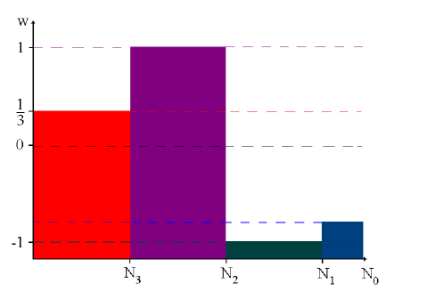
Figure 1: Parameterization of the dark energy evolution

it is shown how this parameterization can be done. In the horizontal axis the e–folds number are calculated now with respect to the present time $N_{0}$, i.e., $N$ increases leftward. In the vertical axis is $w(N)$, which determines the equation of state $p=w\rho$. With dashed lines are denoted four cases where $w$ is a constant: a stiff fluid ($w_{s}=1$), radiation ($w_{R}=1/3$), matter ($w_{M}=0$), a tracker scalar field (which is a special case of quintessence models where $w$ can be safely approximated to be constant with $-1<w_{tracker}<-1/3$), and a cosmological constant ($w_{\Lambda}=-1$). Those cases that do not satisfy the condition $w<-1/3$ get thrown out of the game because they do not produce an accelerated expansion.

More generally, one can look for parameterizations where $w$ can be approximated by different constants for different ranges of e–folds number. In the figure the filled polygons represents case,

$$w(N)=\left\{\begin{array}[]{l}\quad\quad\;\;w_{4}=\frac{1}{3},\quad\quad\quad\quad\,\,N>N_{3}\\ \quad\quad\;\;w_{3}=1,\quad\quad N_{3}\geq N>N_{2}\\ \quad\quad\;\;w_{2}=-1,\quad\,N_{2}\geq N>N_{1}\\ -1<w_{1}<-\frac{1}{3},\quad N_{1}\geq N>N_{0}\end{array}\right.$$ (16)

where $-1<w_{1}<-1/3$. As it is explained in Macorra , this could be the case of some fluid which initially behaves like radiation, at some energy scale condensates into a scalar field with dynamics dominated by its kinetic energy, then undergoes a strong friction changing to a phase of totally potential dominated dynamics and, finally, behaves like a tracker field.

It is interesting to check, for instance, how such a parameterization will modify the CMB spectrum and how it compares to a cosmological constant and to tracker fields. CAMB is a program which permits one to compute the CMB spectrum after specifying a number of parameters including $w_{tracker}$ CAMB. To include the constant in sectors parameterization of $w(N)$ it was necessary to match the values of the energy densities $\rho_{wi}$ at the borders of those sectors,

$$\rho_{wi}(N)=\rho^{eff}_{i}\exp\left[-3(1+w_{i})N\right]\,,$$ (17)

where,

$$\rho^{eff}_{i}=\rho_{0}\exp\left(-3\Delta w_{12}N_{2}\right)\exp\left(-3\Delta w_{23}N_{3}\right)\dots\exp\left(-3\Delta w_{(i-1)i}N_{i}\right)$$ (18)

and $\Delta w_{(i-1)i}=w_{(i-1)}-w_{i}$.

In figure 2,

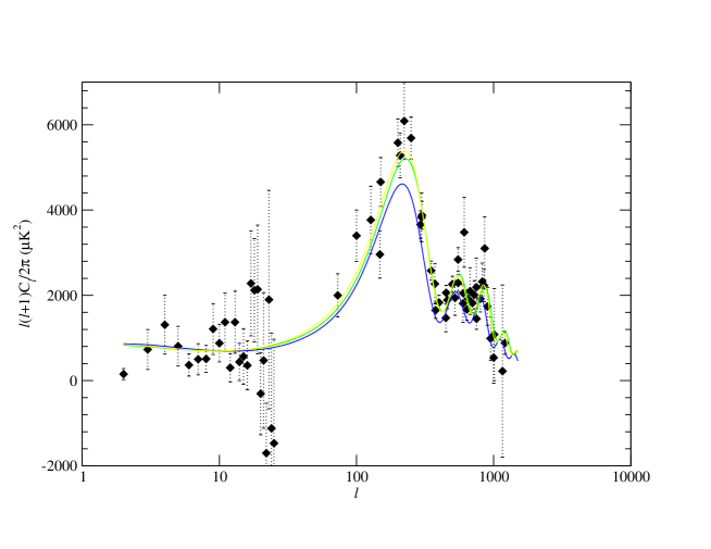
Figure 2: The CMB spectra for different versions of the parametrization by sectors of the state parameter $w$.

examples are presented of the variations of the CMB spectrum after varying the parameters in (16). In this figure the binned data from experiments DASI, Boomerang, MAXIMA and COBE–DMR is also shown. Though a more detailed analysis is still in process, it can be already noted that variation of the values of $N_{1}$, $N_{2}$ and $N_{3}$ modifies the heights and positions of the peaks and dips of the theoretical curve of the CMB spectrum. In fact, one can choose the values of these parameters in such a way that the fit to data might be improved compared to the cases of a cosmological constant and a tracker field as shown in figure 3,

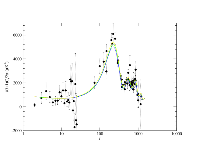
Figure 3: Comparing a tracker field case (blue curve), the $\Lambda$ case (green curve) and a case with $w(N)$ parametrized by sectors (yellow line).

where the blue curve represents the spectrum for a tracker field with $w_{tracker}=-0.86$, the green curve stands for a cosmological constant and the yellow one corresponds to $N_{1}=1.97$, $N_{2}=4.2$, $N_{3}=6.5$ and $w_{1}=-0.86$. Certainly, the data error bars are still too large to make any strong conclusion in this direction but results are encouraging.

4.2 Cosmic Acceleration in the Very Early Universe

As in the case of the present-day Universe, if the acceleration in the very early times –required to solve the SBB problems– is proposed to be induced by the vacuum energy associated with a cosmological constant, then several problems are confronted. The theory of nucleosynthesis, which is so successful in accounting for the observed cosmic abundances of the lightest atoms, describes a radiation–dominated Universe. In this way, in order to reproduce the SBB success, the inflationary period must end some time before nucleosynthesis started. Moreover, if the density perturbations leading to large–scale structure are wanted to be causally seeded by an inflationary period in the very early Universe, then the Hubble radius at some point must start to increase, which implies the end of the accelerated expansion.

Once the energy of a cosmological constant begins to dominate over other non-exotic forms of energy, it will dominate forever. Thus, the inflationary epoch will have no end. Once more, a single scalar field seems to be the simplest candidate to solve all the problems associated with a cosmological constant while still producing enough inflation. In this framework, the origin of the density perturbations leading to LSS is thought to be the quantum fluctuations of the scalar field during inflation inflation ; Bran . A distinguishing feature of this scenario is that, along with the density perturbations associated with the inflaton field, tensor perturbations are also produced which are associated with space–time metric perturbations. All of these fluctuations will be amplified by the accelerated expansion and seeded at the required time through the mechanism of crossing out and crossing back the Hubble horizon. The primordial perturbations are parameterized as,

$$\ln A^{2}(k) = \ln A^{2}(k_{*})+n(k_{*})\ln\frac{k}{k_{*}}$$ (19)

$$+ \frac{1}{2}\frac{d\,n(k)}{d\ln k}|_{k=k_{*}}\ln^{2}\frac{k}{k_{*}}+\cdots\,,$$

where $A$ stands for the normalized amplitudes of the scalar ($A_{S}$) or tensor ($A_{T}$) perturbations, the corresponding spectral indices, $n$, are defined by,

$$n_{S}-1 \equiv \frac{d\ln A_{S}^{2}}{d\ln k}\,,$$ (20)

$$n_{T} \equiv \frac{d\ln A_{T}^{2}}{d\ln k}\,,$$ (21)

and $k=aH$ is the comoving wavenumber corresponding to the wavelength matching the Hubble distance. As it was discussed in the previous chapters of this book, one of the problems of the SBB is the very constrained nature of the initial conditions required for the LSS formation. One of the most restricting requirement is the almost scale invariant nature of the primordial perturbations. Obviously, this impose strong constraints on the values of the parameters in expansion (19). Along with the requirement of yielding a sufficiently large number of e–foldings, $n_{S}\approx 1$ and $n_{T}\approx 0$ are strong conditions to determine whether a proposed scalar field model is a successful inflationary model.

The horizon–flow functions (12) serve as link between observations and the inflationary dynamics. For most inflationary models, exact expressions for parameters in (19) are unknown. The usual way to calculate them is as an expansion in terms of the horizon–flow functions (see Stewart:1993bc ; HFFampl for details). To next–to–leading order in terms of the horizon–flow functions, indices (20) and (21) are written as Stewart:1993bc ; Terrero-Escalante:2002sd

$$n_{S}-1 = -2\epsilon_{1}-\epsilon_{2}-2\epsilon_{1}^{2}-(2C+3)\epsilon_{1}\epsilon_{2}-C\epsilon_{2}\epsilon_{3},$$ (22)

$$n_{T} = -2\epsilon_{1}-2\epsilon_{1}^{2}-2(C+1)\epsilon_{1}\epsilon_{2}\,,$$ (23)

where $C\approx-0.7293$. Dynamics described using the horizon–flow functions correspond to an inflationary potential correspond. This way, the corresponding spectral indices can be calculated and compared with the observational values.

The big problem here is that there exists a large number of single scalar fields models in good agreement with observations, therefore it is difficult to determine which is the one corresponding to the actual physics in the very early Universe. With this aim, a more efficient approach seems to be to constrain and determine the main features of the inflaton potential according to observations, instead of building models and comparing their predictions with the measured data (see Copeland and Easther:2002rw for references on this approach).

Recalling that, according with (12), the definition of $\epsilon_{m+1}$ involves the derivative with respect to $N$ of $\epsilon_{m}$, (22) and (23) are therefore differential equations for $\epsilon_{1}$. In this way, solving these equations and using expression (15), the inflaton potential can be determined from the information on the functional forms of the tensor and scalar spectral indices.

The strong limitation for this program to be useful is that the most that is known (and will be for a while) about the scale or time dependence of the spectral indices is the observed values of a very few parameters in expansions (19), together with the corresponding error bars. Taking this limitation into account, the best one can do is to look for generic features of the potential yielding values of the primordial parameters in agreement with those derived from observations, using some “well based” assumptions for the values of those parameters which have not been observed so far.

For instance, in ConstNt it was proved that if it is assumed $dn/d\ln k=0$ for the scalar and the tensor perturbations, then the resulting potential is an exponential function of the inflaton field. This corresponds to the scenario known as power-law inflation because $a\sim t^{p}$ with $p\gg 1$ PLinfl .

If $dn_{S}/d\ln k\ll 1$ is allowed to be non-zero while keeping $dn_{T}/d\ln k=0$, it can be seen that power–law inflation is an attractor of the corresponding inflationary dynamics ConstNt . This implies that it is difficult to distinguish the actual potential from the exponential one using only the observational information.

A similar result is obtained if both spectral indices are allowed to be scale–dependent but with this dependence being detectible up to the second order on the horizon–flow functions Terrero-Escalante:2001rt .

The role of the tensor perturbations deserves special attention when determining the best–fit values of the cosmological parameters from CMB and LSS spectra. That is motivated in part by the possibility of measuring the cosmic background polarization inflation , allowing the tensorial contribution to be indirectly determined. This contribution can be parametrized in terms of the relative amplitudes of the tensor and scalar perturbations,

$$r\equiv\alpha\frac{A_{T}^{2}}{A_{S}^{2}}\,,$$ (24)

where $\alpha$ is a constant. The expectation is to measure a central value of $r$. Thus the question is how look like the inflationary dynamics yielding an almost constant ratio $r$. The answer was given in Terrero-Escalante:2001du where it was shown that in the case of an exactly constant $r$, power–law inflation is a repulsor of the corresponding dynamics. Since it describes a quick and strong depart from scale–invariance, for the model to be successful, the perturbations must be produced in the quasi power–law regime, once more making it difficult to observationally distinguish between the two dynamics.

All of the above-discussed results imply a serious handicap for any program of reconstruction of the inflaton potential. A way to improve this situation, could be to combine the information on $\Delta n$ (the difference between the spectral indices) and the value of $r$, with the two first horizon–flow functions Terrero-Escalante:2002uj . It follows from definitions (20), (21) and (24) that

$$\frac{d\ln r}{d\ln k}=\Delta n\equiv n_{T}-(n_{S}-1)\,,$$ (25)

this way, any information on the evolution of both spectral indices can be used as information on the scale dependence of the tensor to scalar ratio.

With regards to these, it becomes important to analyze in details the case,

$$\ln\frac{r}{16}=a_{0}+a_{1}(N-N_{0})\,,$$ (26)

where the corresponding solution for $\epsilon_{1}$ is Terrero-Escalante:2002uj ,

$$\epsilon_{1}(N)=\epsilon_{1(i)}\exp\left[B\exp\left(-\frac{N}{C}\right)\right]\exp\left(AN\right)\,,$$ (27)

with $\epsilon_{1(i)}\equiv\epsilon_{1(0)}\exp\{\left[a_{0}+\left(N_{0}-C\right)a_{1}\right]C\}$ and $A\equiv a_{1}C$. The asymptotes of this solution for $B\neq 0$ will be mainly determined by the value and sign of $B$. However, for $A=0$ (i.e., $\ln r/16=a_{0}$), if the model yielding $\epsilon_{1}$ given by (27) is expected to be compatible with current data, $B$ has to be chosen an extraordinarily small number. Once more, this will make it very difficult to observationally distinguish the corresponding scenario from power–law inflation. More interesting is the case $B=0$ where the potential is,

$$V=V_{0}\left(3-\frac{A^{2}}{4}\psi^{2}\right)\exp\left(-\frac{A}{2}\psi^{2}\right)\,,$$ (28)

with $\psi\equiv\sqrt{\kappa/2}(\phi+\phi_{0})$. In Fig. 4

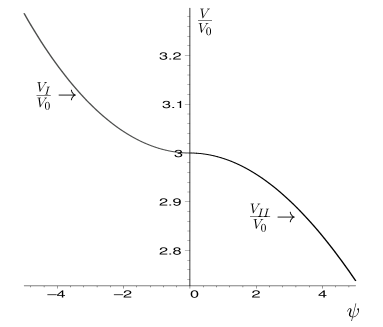
Figure 4: Sectors of the inflaton potential given by (28) for $A=-0.0073$ ($V_{I}$) and $A=0.0073$ ($V_{II}$).

sectors of this potential are plotted for $A=-0.0073$ ($V_{I}$) and $A=0.0073$ ($V_{II}$). For this model, information on the existence of extrema and on the curvature can be derived. As can be seen in Fig. 4, realizations of this potential resemble the cases of monomial potentials with even order ($V_{I}$, $\epsilon_{2}<0$), and inflation near a maximum ($V_{II}$, $\epsilon_{2}>0$) (see inflation for examples of such inflationary scenarios motivated by particles physics) allowing, therefore, to observe features of the inflaton potential beyond the exponential form characteristic of power–law inflation. In Terrero-Escalante:2002uj it was shown that for a large set of $A$ and $\epsilon_{1(i)}$ values, the corresponding spectra agree with CMB and LSS observations.

On the Order of the Approximations

A crucial question in the analysis in the previous section is to what extent these results depend on the order of expressions underlying the calculations. It is widely believed that this is not of concern. Let us show that it must be.

To next–to–next–to–leading order the tensor to scalar ratio is given by,

$$\ln\frac{r}{r_{0}} = \ln\epsilon_{1}+C\epsilon_{2}+\left(-\frac{\pi^{2}}{2}+5+C\right)\epsilon_{1}\epsilon_{2}$$ (29)

$$+ \left(-\frac{\pi^{2}}{8}+1\right)\epsilon_{2}^{2}+\left(-\frac{\pi^{2}}{24}+\frac{C^{2}}{2}\right)\epsilon_{2}\epsilon_{3}\,.$$

If the order of this expression was of little concern, then the corresponding solution for the case with $r$ given by (26) must be very similar to potential (28). To check this, one can assume,

$$\epsilon_{1}=\epsilon_{1}^{nlo}\left(1+\delta\right)\,,$$ (30)

with $\delta<<1$, yielding

$$\epsilon_{2} = \epsilon_{2}^{nlo}+\frac{d\delta}{dN}$$ (31)

$$\epsilon_{2}\epsilon_{3} = \epsilon_{2}^{nlo}\epsilon_{3}^{nlo}+\frac{d^{2}\delta}{dN^{2}}\,,$$ (32)

where the super-index $nlo$ stands for the next-to-leading order solution. $\delta(N)$ is expected to remain very small as $N$ increases. Substituting (30), (31) and (32) into (29) with $\epsilon_{1}^{nlo}$ given by expression (27) it is obtained that

$$\frac{d^{2}\delta}{dN^{2}} + D(N)\frac{d\delta}{dN}+S(N)\delta=F(N)$$ (33)

$$D(N) = C_{3}+C_{2}\epsilon_{1(i)}\,{e^{B{e^{NC_{1}}}}}{e^{AN}}$$ (34)

$$S(N) = -C_{4}+C_{2}\epsilon_{1(i)}\,{e^{B{e^{NC_{1}}}}}{e^{AN}}\left(C_{1}B{e^{NC_{1}}}+A\right)$$ (35)

$$F(N) = C_{2}\epsilon_{1(i)}\,{e^{B{e^{NC_{1}}}}}{e^{AN}}\left(C_{1}B{e^{NC_{1}}}+A\right)+C_{5}B{e^{NC1}}+C_{6}A\,,$$ (36)

where non-linear terms of $\delta$ were neglected and $C_{i}$ (with $i=1\dots 6$) are fixed constants given in terms of $C$ and $\pi$. Constants $\epsilon_{1(i)}$, $A$ and $B$ are those already given in the next–to–leading order solution (27). In Figs. 5, 6 and 7 the $N$-dependent parameters $D(N)$, $S(N)$ and $F(N)$ are plotted for the same numerical values for the constants used in Terrero-Escalante:2002uj .

Figure 5: The behavior of D(N) for $A=-0.0073$ and $\epsilon_{1(i)}=0.05$.

Figure 6: The behavior of S(N) for $A=-0.0073$ and $\epsilon_{1(i)}=0.05$.

Figure 7: The behavior of F(N) for $A=-0.0073$ and $\epsilon_{1(i)}=0.05$.

At least for this case, the parameters can be safely approximated by constants. Therefore, a qualitative analysis of the phase space for the flow given by (33) can be carried out. It yields that there exists a saddle point at $(\delta=F/S,\dot{\delta}=0)$, shown in figure 8.

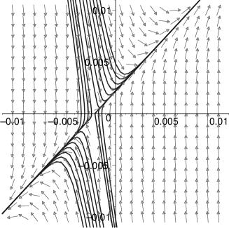
Figure 8: The phase portrait for (33) with $D=-5.32$, $S=6.891$ and $F=0.014$. In the horizontal axis $\delta$ is represented; in the vertical axis, $\dot{\delta}$. Arrows show the vector field and lines some trajectories.

It means that solutions for $\delta(N)$ with $A=-0.0073$ and $\epsilon_{1(i)}=0.05$ are likely unstable. A more complete analysis is indeed required, but this result would serve as a warning to pay more attention to the order of the approximations used when information on the inflationary dynamics is drawn from observational data.

5 Conclusions

Cosmic acceleration is a trivial solution to the Einstein equations for an isotropic and homogeneous Universe, as appears to be the one where we live. An accelerated expansion is typical of Universes filled with a kind of energy yielding a strong enough negative pressure. This is the case when the cosmic energy is dominated by the contribution of the vacuum.

Observational evidence strongly suggest that our Universe’s evolution includes three well-defined epochs with regards to the increase of the cosmic volume. First, the very early Universe would undergo an accelerated expansion known as inflation. Then, a period of non-accelerated expansion would take place where most of the known kinds of matter and matter structures were formed. Finally, in recent times (with respect to cosmic scales) the Universe would enter a second epoch of accelerated expansion where the corresponding dominated matter-energy content is called dark energy.

A real scalar field is a good candidate for inducing cosmic acceleration. It may help to solve problems arising when a constant vacuum energy is used to explain inflation or the nature of the dark energy. For the required negative pressure, the scalar field dynamics must be dominated by its potential energy.

A hot question in cosmology is whether the observed (predicted) cosmic acceleration is (was) induced by a scalar field. If this is the case, the relevant question is to determine the origin and nature of the corresponding potential. This will open an important window into high energy physics.

Here, an idea was hinted at on how to differentiate between candidates for the dark energy. The proposal is to divide the evolution of the dark energy in periods where the corresponding equation of state could be approximated to be linear. The best–fit values for the corresponding slopes would indicate the favorite candidate. Encouraging results have been obtained in this direction.

It was also explained some of the difficulties that arise when deriving the inflationary potential from observations. It seems like the best that can be done is to indicate generic features of the potentials yielding perturbations spectra matching the measured data. It was emphasized that the use of data on the difference of the tensor and scalar indices of perturbations yields information on the scale–dependence of the tensor to scalar ratio of primordial perturbation amplitudes. This information may be very useful in classifying the inflationary potentials. Finally, a warning was issued about the possibility that the features of the inflaton potential drawn from the observational data could be biased by the order of the approximations used to derive the expressions underlying the calculations.

Acknowledgments

I would like to thank School organizers for inviting me to give this talk. I also thank A. García, A. de la Macorra and A. Coley for their solid support and helpful discussions. Supported in part by CONACyT grant 38495–E and SNI (Mexico).

References

- (1) J. L. Cervantes–Cota: An introduction to standard cosmology, contribution to this book.
- (2) A. R. Liddle and D. H. Lyth: Cosmological Inflation and Large-Scale Structure, 1st edn (Cambridge University Press, Cambridge, 2000).
- (3) A. Filippenko: The accelerating Universe and dark energy: evidence from Type Ia supernovae, contribution to this book [arXiv:astro-ph/0309739].
- (4) A. de la Macorra: Quintessence and dark Energy, contribution to this book.
- (5) E. Copeland: Inflation in the early Universe and today, contribution to this book.
- (6) D. J. Schwarz, C. A. Terrero-Escalante and A. A. Garcia: Phys. Lett. B 517, 243 (2001) [arXiv:astro-ph/0106020].
- (7) R. Brandenberger: Lectures on the theory of cosmological perturbations, contribution to this book [arXiv:hep-th/0306071].
- (8) C. A. Terrero-Escalante and A. A. Garcia: Phys. Rev. D 65 023515 (2002) [arXiv:astro-ph/0108188].
- (9) E. Ayon-Beato, A. Garcia, R. Mansilla and C. A. Terrero-Escalante: Phys. Rev. D 62 103513 (2000) [arXiv:astro-ph/0007477].
- (10) K. Freese and M. Lewis, Phys. Lett. B 540, 1 (2002) [arXiv:astro-ph/0201229].
- (11) A. Y. Kamenshchik, U. Moschella and V. Pasquier, Phys. Lett. B 511, 265 (2001) [arXiv:gr-qc/0103004].
- (12) E. D. Stewart and D. H. Lyth: Phys. Lett. B 302 171 (1993) [arXiv:gr-qc/9302019].
- (13) C. A. Terrero-Escalante: Is power-law inflation really attractive? In Proceedings of IV DGFM-SMF Workshop on Gravitation and Mathematical-Physics, ed by N. Bretón, J. Cervantes and M. Salgado (2001), arXiv:astro-ph/0204066.
- (14) R. Easther and W. H. Kinney, Phys. Rev. D 67, 043511 (2003) [arXiv:astro-ph/0210345].
- (15) C. A. Terrero-Escalante, E. Ayón-Beato, and A. A. Garcia: Phys. Rev. D 64, 023503 (2001).
- (16) F. Lucchin and S. Matarrese: Phys. Rev. D 32, 1316 (1985).
- (17) C. A. Terrero-Escalante, J. E. Lidsey and A. A. Garcia: Phys. Rev. D 65 083509 (2002) [arXiv:astro-ph/0111128].
- (18) C. A. Terrero-Escalante, Phys. Lett. B 563, 15 (2003) arXiv:astro-ph/0209162.