The subhalo populations of $\Lambda$CDM dark haloes

Abstract

We investigate the subhalo populations of dark matter haloes in the concordance $\Lambda$CDM cosmology. We use a large cosmological simulation and a variety of high resolution resimulations of individual cluster and galaxy haloes to study the systematics of subhalo populations over ranges of 1000 in halo mass and 1000 in the ratio of subhalo to parent halo mass. The subhalo populations of different haloes are not scaled copies of each other, but vary systematically with halo properties. On average, the amount of substructure increases with halo mass. At fixed mass, it decreases with halo concentration and with halo formation redshift. These trends are comparable in size to the scatter in subhalo abundance between similar haloes. Averaged over all haloes of given mass, the abundance of low mass subhaloes per unit parent halo mass is independendent of parent mass. It is very similar to the abundance per unit mass of low mass haloes in the universe as a whole, once differing boundary definitions for subhaloes and haloes are accounted for. The radial distribution of subhaloes within their parent haloes is substantially less centrally concentrated than that of the dark matter. It varies at most weakly with the mass (or concentration) of the parent halo and not at all with subhalo mass. It does depend on the criteria used to define the subhalo population considered. About $90$ per cent of present-day subhaloes were accreted after $z=1$ and about $70$ per cent after $z=0.5$. Only about $8$ per cent of the total mass of all haloes accreted at $z=1$ survives as bound subhaloes at $z=0$. For haloes accreted at $z=2$, the survival mass fraction is just 2 per cent. Subhaloes seen near the centre of their parent typically were accreted earlier and retain less of their original mass than those seen near the edge. These strong systematics mean that comparison with galaxies in real clusters is only possible if the formation of the luminous component is modelled appropriately.

The subhalo populations of $\Lambda$CDM dark haloes

1 Introduction

According to the standard CDM scenario, structure in our Universe formed hierarchically. Small-scale fluctuations were the first to collapse as virialised objects. These then merged to form larger systems. The inner regions of early virialised objects are very compact and often survive accretion onto a larger system to become self-bound subhaloes of their host. Since galaxies form by the condensation of gas at the centres of early haloes, most cluster galaxies may well be associated with subhaloes in their host cluster. Only in recent years have numerical techniques and computer capabilities advanced to the point where it is possible to study in detail the properties of such subhaloes (Moore et al. 1998, 1999; Tormen, Diaferio & Syer 1998; Klypin et al. 1999a,b; Ghigna et al. 1998, 2000; Springel et al. 2001; Stoehr et al. 2002, 2003). These studies indicate that the ‘overmerging’ problem in early simulations, i.e. the failure to resolve subhaloes corresponding to galaxies in cosmological simulations of cluster haloes, was in part a result of insufficient mass and force resolution.

Using high resolution resimulations of individual cluster or galaxy haloes, it is possible to study the properties of subhaloes in detail. Recent papers by De Lucia et al. (2004), Diemand et al. (2004) and Gill, Knebe & Gibson (2004) discuss many aspects of this topic and present results compatible with but complementary to those presented below. Most studies to date have been limited because their analysis has been performed on a small number of individual haloes. Since halo-to-halo variations are large, this may prevent the derivation of statistically significant results. In addition, all studies are still affected at some level by numerical resolution. The available tests show that the subhaloes seen in a particular object are reproduced moderately well in mass, but not in position or velocity, when the same object is resimulated multiple times with varying resolution (Ghigna et al. 2000; Springel et al. 2001; Stoehr et al 2002, 2003). This is a result of the well known divergence of neighboring trajectories in nonlinear dynamical systems.

In this paper, we carry out a systematic study of the properties of subhaloes in the halo population of a single, large-scale cosmological simulation, and we complement this by analysing a multi-resolution set of resimulations of a single ‘Milky Way’ halo, together with a set of high-resolution resimulations of eight different rich clusters. These resimulations allow us to investigate how numerical resolution and halo-to-halo variation affect the conclusions from our cosmological simulation. We do not, however, carry out a full study of the numerical requirements for fully converged numerical results for the properties of subhaloes.

Previous studies of subhaloes within haloes of different scale have emphasised similarities – to a large extent the internal structure of a ‘Milky Way’ halo looks like a scaled version of that of a rich cluster halo (Moore et al. 1999; Helmi & White 2001; Stoehr et al. 2003; De Lucia et al. 2004; Desai et al. 2004). We show below that this scaling is not exact, and that a better model assumes the mass distribution of low-mass subhaloes to be the same as in the Universe as a whole, once the differing definitions of an object’s boundary are accounted for. We show that galaxy haloes have fewer high-mass subhaloes than rich clusters because of their earlier formation times. Indeed, even among haloes of given mass, the number of massive subhaloes correlates well with formation time, as reflected in the halo’s central concentration.

The emphasis of earlier high resolution work on solving the ‘overmerging problem’ has given rise to the impression that the subhaloes are typically objects which formed at very early times. We demonstrate below that this is not the case. Even at low subhalo masses, most subhaloes were accreted onto the main halo at low redshift, in most cases well below $z=1$. This is important when considering the formation paths of present-day cluster galaxies.

Our paper is organized as follows. We introduce our various simulation sets in Section 2. In Section 3, we compare the halo mass abundance function measured from our cosmological simulation with theoretical predictions and with earlier numerical data. In Section 4, we investigate the subhalo population as a function of halo mass and of redshift. The spatial distribution of subhaloes within haloes is also discussed in Section 4. In Section 5 we investigate the infall and mass-loss histories of present-day subhaloes, as well as the fate of objects that are accreted onto bigger clusters at early times. We discuss our results and set out our conclusions in Section 6.

2 The Simulations

2.1 The GIF2 cosmological simulation

We have carried out a cosmological simulation of a $\Lambda$CDM universe in a periodic cube of side 110 $h^{-1}$Mpc. The total number of particles is $400^{3}$, and the individual particle mass is $1.73\times 10^{9}h^{-1}{\rm M\odot}$. This is a factor of 8 better than the mass resolution of the GIF simulations published by Kauffmann et al. (1999) but otherwise the parameters and output strategy of the simulations are rather similar. We therefore call our new simulation GIF2. The cosmological parameters adopted are: $\Omega=0.3$, $\lambda=0.7$, $\sigma_{8}=0.9$, and $h=0.7$; We choose initial fluctuation power spectrum index $n=1$, with the transfer function produced by CMBFAST (Seljak & Zaldarriaga 1996) for $\Omega_{b}h^{2}=0.0196$.

Initial conditions were produced by imposing perturbations on an initially uniform state represented by a ‘glass’ distribution of particles. This we generated with the method developed by White (1993) which involves evolution from a Poisson distribution with the sign of Newton’s constant changed when calculating peculiar gravitational forces. Fluctuations are imposed using the algorithm described in Efstathiou et al. (1985). Based on the Zeldovich (1970) approximation, a Gaussian random field is set up by perturbing the positions of the particles and by assigning them velocities according to the growing mode solution of linear theory.

In order to save computational time, we performed the simulation in two steps. First, we ran the simulation from high redshift until $z=2.2$ with the parallel SHMEM version of HYDRA (Couchman, Thomas & Pearce 1995; Macfarland et al. 1998). At these times the particle distributions are lightly clustered and thus the P3M based gravity solver is quite efficient. We then completed the simulation with a tree-based parallel code, GADGET (Springel, Yoshida & White 2001), which has better performance in the heavily clustered regime.

Since the two codes adopt different force-softening schemes, it is necessary to match the force shape at the time we switch from one code to the other. The softened force becomes Newtonian at a distance of about $2.3\epsilon$ for HYDRA, while this occurs at a distance of $2.8\epsilon$ for GADGET. Experimentation showed that a factor of 1.06, namely $\epsilon_{\rm Hydra}=1.06\epsilon_{\rm Gadget}$, produces an excellent match of the two force laws. In practice, we started the simulation at $z=49$ with $\epsilon=7h^{-1}$kpc in comoving units within HYDRA, and changed the softening to $\epsilon=6.604h^{-1}$kpc for the continuation with GADGET after redshift 2.2.

The simulation was carried out on 512 processors of the Cray T3E at the Rechenzentrum Garching, the supercomputer centre of the Max-Planck Society. We stored the data at 50 output times logarithmically spaced between $1+z=20$ and $1+z=1$. This enables us to construct halo and subhalo merging trees as in Springel et al (2001). These will be used in other work to model galaxy formation within the simulation, so that issues of galaxy assembly and galaxy clustering can be addressed. The numerical data for our GIF2 simulation are publicly available at http://www.mpa-garching.mpg.de/Virgo

2.2 Higher resolution simulations of individual halos

In order to investigate the importance of numerical and resolution effects in the study of subhaloes, we have used a set of multi-resolution resimulations of a Milky Way sized halo carried out by Stoehr et al. (2002, 2003). The simulations studied here are the versions called GA1, GA2 and GA3n in the original papers. The final mass of the main halo studied here is $M_{200}=2\times 10^{12}h^{-1}{\rm M_{\odot}}$ and its maximum circular velocity is 240 ${\rm km}s^{-1}$. In this series of resimulations all perturbation modes present in the initial conditions of a given resimulation are exactly inherited by all higher resolution ones. Hence all significant structure in the low resolution systems should be reproduced at higher resolution. The number of particles in the high-resolution region, the particle mass and the gravitational softening are given for the GA simulations in Table 1.

We analyse in addition a set of 8 high-resolution resimulations of rich cluster halos previously studied in Gao et al. (2004a) and Navarro et al. (2003). These simulations all have the same particle mass and force resolution, $5.12\times 10^{8}h^{-1}{\rm M_{\odot}}$ and $\epsilon=5h^{-1}$kpc, respectively. The clusters were originally chosen as all objects in a relatively narrow mass range within the $0.479h^{-1}$Gpc cosmological simulation of Yoshida et al. (2001). The initial particle number in the high resolution region of each simulation and the mass of the final virialized object are listed in Table 2.

All these high-resolution resimulations assumed the same cosmological parameters as our GIF2 simulation, and all were all run with the publicly available code Gadget 1.1.

Table 1: Numerical parameters for the GA-series simulations.

	$GA0$	$GA1$	$GA2$	$GA3n$
$N_{p}$	68323	637966	5953033	55564205
$m_{p}[h^{-1}{\rm M_{\odot}}]$	$1.8\times 10^{8}$	$1.9\times 10^{7}$	$2.0\times 10^{6}$	$2.5\times 10^{5}$
$\epsilon[h^{-1}{\rm kpc}]$	1.8	1.0	0.48	0.24

Table 2: Particle number in the high resolution region and final $M_{200}$ for the 8 cluster simulations.

	$C1$	$C2$	$C3$	$C4$	$C5$	$C6$	$C7$	$C8$
$N_{p}$	8457516	7808951	13466254	9352943	9011020	8704054	10182210	8454580
$m_{200}[h^{-1}{\rm M_{\odot}}]$	$0.81\times 10^{15}$	$0.75\times 10^{15}$	$0.52\times 10^{15}$	$0.54\times 10^{15}$	$0.62\times 10^{15}$	$0.84\times 10^{15}$	$0.45\times 10^{15}$	$0.60\times 10^{15}$

3 The mass function of haloes

We have used a friends-of-friends group-finding algorithm (Davis et al. 1985) with the standard linking length of 0.2 in units of the mean interparticle separation to identify virialised haloes in our GIF2 simulation. Only haloes which contain at least 20 particles are included in the halo catalogues we analyse below.

The halo mass function (the abundance of haloes as a function of their mass) is one of the fundamental quantities characterising the nonlinear distribution of mass in the Universe. Substantial effort has gone into building theoretical models for this function and into calibrating them with numerical simulations (Press & Schechter 1974; Bond et al. 1991; Lacey & Cole 1993, 1994; Mo & White 1996; Sheth & Tormen 1999; Sheth, Mo & Tormen 2001; Jenkins et at. 2001; Reed et al. 2003; Yahagi et al. 2004). Here we use our GIF2 simulation, which has a reasonable volume and good mass resolution, to compare the FOF halo mass distribution against published fitting formulae for halo masses down to $4\times 10^{10}h^{-1}{\rm M_{\odot}}$ and for redshifts up to $z=5$.

In Fig. 1, we plot the differential halo mass function measured directly from the GIF2 simulation (red dotted line), the theoretical predictions from Press-Schechter theory (dotted line) and from Sheth & Tormen(1999)(dashed line), and the fit to numerical data published by Jenkins et al. (solid line). Note that we plot the mass function of Jenkins et al. only over the mass range where their fitting formula was checked. We have multiplied the mass function by $M^{2}$ before plotting in order to take out the dominant mass dependence and to make the differences between the various formulae more apparent. Fig. 1 clearly shows that, in the redshift and mass range studied, the FOF(0.2) halo mass function is well described by the formulae of Jenkins et al. and of Sheth & Tormen. While being not perfect, the fit is extremely good in comparison with the Press & Schechter mass function. This confirms the recent conclusion of Reed et al. (2003) and Yahagi et al. (2004), based on simulations of smaller volumes, that these formulae can be applied at earlier redshift and to lower masses than previously demonstrated.

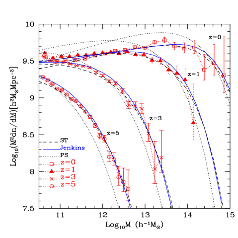
Figure 1: Comparison of the differential halo mass function in our GIF2 simulation with different analytic predictions. Halos were identified with a standard FOF algorithm with linking length $b=0.2$, and we plot data for all haloes containing more than 20 particles. Note that we have multiplied the mass function by $M^{2}$ to take out the dominant mass dependence.

Figure 2: Differential subhalo abundance functions per unit host mass for the final haloes in our GA1, GA2 and GA3n simulations. Error bars assume Poisson uncertainties in the counts.

4 Subhalo populations

Several methods have been proposed to identify subhaloes within larger systems. For a detailed review we refer to Springel et al. (2001; hereafter SWTK). In this paper, we use the algorithm SUBFIND, developed by SWTK, to isolate locally overdense and self-bound particle sets within dark matter haloes. All such subhaloes containing at least 10 particles are included in our subhalo catalogues.

4.1 A convergence study of subhalo populations

Independent of the particular method employed to identify subhaloes, most published studies agree that the differential subhalo mass function (MDF) of an individual halo is approximately a power-law, $dn/dm\sim m^{-\alpha}$, with $\alpha=1.7-1.9$ independent of redshift and of the mass of the parent halo (Moore et al. 1999; Ghigna et al. 2000; De Lucia et al. 2004). No study so far has compared in detail the properties of the subhaloes identified by different methods. Different criteria for defining the boundaries and the membership of subhaloes are bound to lead to systematic differences in subhalo populations, but the uniformity of the derived slopes suggests that such differences may be correctable through simple scaling factors.

Further study of the effects of numerical resolution on simulated subhalo populations is clearly important. Numerical convergence was claimed by Ghigna et al. (2000; hereafter G00), by SWTK and by Stoehr et al (2002, 2003) on the basis of multi-resolution simulations of individual objects. However, the data presented are not fully convincing. For example, Fig. 5 of SWTK shows the subhalo mass function for a rich cluster resimulated 4 times with increasing mass and force resolution. The subhalo abundance in the lowest resolution simulation S1 agrees well with that in the highest resolution simulation S4, while the intermediate resolution simulations S2 and S3 agree very well with each other but appear significantly offset from S4. The reasons for this are unclear. We show similar data in Fig. 2 for the subhalo abundance in the GA series resimulations of a ‘Milky Way’ halo. (A cumulative version of this plot is given by Stoehr et al. (2002) but without GA3n data). Here agreement is excellent for subhaloes that contain at least 30 particles, but there may be significant differences for smaller subhaloes. These could be due to resolution problems. As we show below (Section 4.6 and Fig. 10) it appears that subhaloes with small $N$ dissolve overly fast, particularly in the inner regions of a halo.

In order to avoid effects due to our particular definition of the boundary of a subhalo (and so of its mass) we check this convergence by examining the abundance of haloes in our GA series as a function of their maximum circular velocity $V_{\rm max}$. We define the square of this quantity to be the maximum value of $GM(r)/r$ for those particles identified as bound to the subhalo by SUBFIND. $V_{\rm max}$ is a more stable quantity than the subhalo mass and depends little on how the subhalo is defined. Fig. 3 demonstrates that the cumulative abundance of subhaloes as a function of $V_{\rm max}$ (the VDF) is very well reproduced between the different simulations in the GA series. Thus, we conclude that our simulation techniques correctly reproduce the subhalo abundance down to objects of relatively small particle count. In particular, GA3n reproduces the correct subhalo abundance down to values of $V_{\rm max}$ below 10 km/s and so well below the values relevant to the observed satellites of the Milky Way.

Figure 3: The cumulative abundance of subhaloes as a function of maximum circular velocity $V_{\rm max}$ for the final haloes in the GA1, GA2 and GA3n simulations.

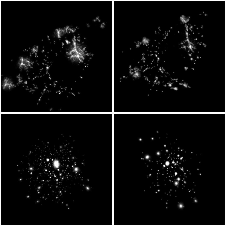
Figure 4: Images at $z=0$ and $z=5$ of the material contained in $z=0$ subhaloes of the main halo with mass exceeding $5.8\times 10^{8}h^{-1}{\rm M_{\odot}}$ in GA2 and GA3n. Upper plots are for $z=5$, lower plots for $z=0$. GA2 is shown on the left and GA3n on the right.

Dark matter haloes are strongly nonlinear and chaotic N-body systems, so we cannot expect simulations of the ‘same’ object run with different resolution, with different codes, or with different integration parameters to be very similar at the final time. (See for example the various simulations from identical initial conditions in the Santa Barbara Cluster Comparison Project (Frenk et al. 1999) This is because in a chaotic N-body system any small perturbation to the trajectory is amplified exponentially by subsequent evolution. In the bottom panel of Fig. 4, we show density maps for all subhaloes belonging to the final FOF haloes of GA2 (left-hand panel) and GA3n (right-hand panel). Although these plots are qualitatively similar, there is no detailed correspondance between subhaloes. On the other hand, the upper panels show that the material which makes up these subhaloes is very similarly distributed in the two simulations at early epochs. The biggest differences are due to subhaloes which are included in the final halo in one of the simulations but are just outside it in the other. Fortunately, we do not care much about the positions of individual subhaloes and are more interested in statistical results. A re–simulation of an object with higher resolution may not reproduce its structure in detail, but it can still be viewed as the result of evolution from a nearby set of initial conditions (e.g. Hayes 2003).

4.2 Is the population of subhaloes similar in all haloes?

A number of authors have argued that the statistical properties of subhaloes in a galaxy-sized halo are simply a scaled version of those in a rich cluster halo (Moore et al. 1999; Helmi & White 2001; De Lucia et al. 2004; Diemand et al. 2004). Prima facie this is surprising, since it is well known that the merging histories of haloes (and in particular their formation times) vary systematically with mass (Lacey & Cole 1993; Navarro, Frenk & White 1997). One might expect these differences to result in a systematic dependence of the subhalo population on mass.

Figure 5: Mass functions at $z=0$ for subhaloes within radius $r_{200}$ of their parent haloes. In the top left-hand panel we plot differential subhalo abundance as a function of scaled subhalo mass, $m_{n}=m_{\rm sub}/M_{\rm halo}$, for three ranges of halo mass in our GIF2 simulation, for GA3n and for our 8 cluster resimulations. In the top right-hand panel, we plot the corresponding cumulative mass functions. In the bottom left-hand panel, we plot differential subhalo abundance normalized to the total mass of the parent haloes, $\langle M_{\rm halo}dn/dm_{\rm sub}\rangle$. The corresponding cumulative mass functions are shown in the bottom right-hand panel.

We define a dimensionless subhalo mass, $m_{n}=m_{sub}/M_{\rm halo}$, where $M_{\rm halo}$ is the virial mass of the parent halo defined as spherical region which has 200 times critical density of universe at that time. In the upper panels of Fig. 5, we plot subhalo abundance against this normalized mass for three ranges of halo mass in our GIF2 simulation, $[3\times 10^{14}h^{-1}{\rm M_{\odot}},\ 10^{15}h^{-1}{\rm M_{\odot}}]$, $[10^{14}h^{-1}{\rm M_{\odot}},\ 3\times 10^{14}h^{-1}{\rm M_{\odot}}]$ and $[3\times 10^{13}h^{-1}{\rm M_{\odot}},\ 10^{14}h^{-1}{\rm M_{\odot}}]$. These bins contain 7, 33 and 243 haloes, respectively. In this plot we also include subhalo abundance functions for GA3n and for our 8 cluster simulations. If halo populations of differing mass were just scaled copies of each other, these various abundance functions would all agree. In fact, however, the differential and cumulative normalized mass functions of Fig. 5 depend systematically on halo mass. The subhalo abundance in high-mass haloes is clearly higher (at given scaled subhalo mass) than in low-mass haloes. The difference between the rich cluster haloes and the galaxy halo GA3n is a factor of 2. The cluster haloes also clearly have more abundant subhaloes than the lowest mass haloes in our GIF2 simulation. Our simulation data agree with semi-analytical modelling by Zentner & Bullock (2003). These authors argued that, on average, the subhalo mass fraction should increase with halo mass because high mass haloes were assembled more recently. A trend in this direction is also clearly present in in high resolution simulation data of Diemand et al. (2004), although these authors emphasise the similarity in subhalo abundance between cluster and galaxy halo rather than the difference.

In the bottom panels of Fig. 5, we show differential and cumulative plots of subhalo mass abundance using a different normalization procedure. We divide the total number of subhaloes in each bin by the total mass of all the parent haloes to obtain the subhalo abundance per unit parent halo mass. We then plot this abundance as a function of the actual mass (rather than the scaled mass). With this normalization, the subhalo mass functions of different mass haloes agree very well (see also Kravtsov et al. 2004a). For relatively low-mass parent haloes the subhalo abundance drops below that seen in more massive parent haloes for subhalo masses exceeding about 1 per cent of the parent mass. Ignoring this high mass cut-off, the subhalo abundance per unit halo mass in Fig. 2 is reasonably well fit by:

$$dn/dm\simeq 10^{-3.2}(m_{\rm sub}h/{\rm M_{\odot}})^{-1.9}h{\rm M_{\odot}}^{-1}$$ (1)

An immediate consequence of the universality of this relation is a shift with parent halo mass in the abundance of subhaloes as a function of scaled mass $m_{n}$. For small subhalo masses this shift is

$$\triangle\log_{10}f(m_{n};M_{\rm halo})=0.1\triangle\log_{10}M_{\rm halo}\,,$$ (2)

where $f(m_{n};M_{\rm halo})$ is the mean abundance of subhaloes by normalized mass $dn/dm_{n}$ in parent haloes of mass $M_{\rm halo}$. Since the slope of the subhalo MDF is close to 2, this shift in the normalized function is quite small. As an example, the abundance shifts by about a factor of 2 at fixed $m_{n}$ between a typical galaxy halo of mass $10^{12}h^{-1}{\rm M_{\odot}}$ and a rich cluster halo of mass $10^{15}h^{-1}{\rm M_{\odot}}$. This is indeed the shift seen between GA3n and the clusters in the upper panels of Fig. 5

In Fig. 6, we plot the abundance of subhaloes as a function of $V_{\rm max}$ for GIF2 haloes in our three mass bins and for our 8 clusters. We normalize the abundance as above by dividing the total subhalo count in each bin by the total mass of the contributing haloes. This figure confirms the result of Fig. 5. With this normalization the subhalo abundance as a function of $V_{\rm max}$ is ‘universal’, i.e. appears not to depend on parent halo mass. We also plot in Fig. 6 the differential abundance of haloes in our GIF2 simulation as a function of $V_{\rm max}$. Here we normalize by the total mass in the simulation. This shows the interesting result that subhalo abundance and parent halo abundance follow similar curves, but with the subhaloes shifted to lower velocity by 20 or 30 per cent. We will come back to this in the next section. Note that the turn-over and drop at small $V_{\rm max}$ for all these curves are due to the resolution limit of the simulations.

Figure 6: Differential abundance of subhaloes as a function of maximum circular velocity $V_{\rm max}$. Curves are shown for three halo mass ranges in the GIF2 simulation and for our 8 cluster simulations. All subhaloes within $r_{200}$ of their hosts are counted, and the number of subhaloes in each bin is normalized by the total mass of the contributing haloes. The curve labelled GIF2 is the corresponding function for the main haloes themselves and is normalized by the total mass in the GIF2 simulation.

Figure 7: The fraction of halo mass in subhaloes. This plot shows the fraction of the mass within $r_{200}$ of halo centre which is in subhaloes more massive than $m_{\rm sub}$ for GIF2 and cluster haloes in our three mass ranges. Error bars on selected points show the rms scatter of the individual values of the mean for the 15 haloes used to derive the curve for the most massive bin.

4.3 The mass fraction in subhaloes

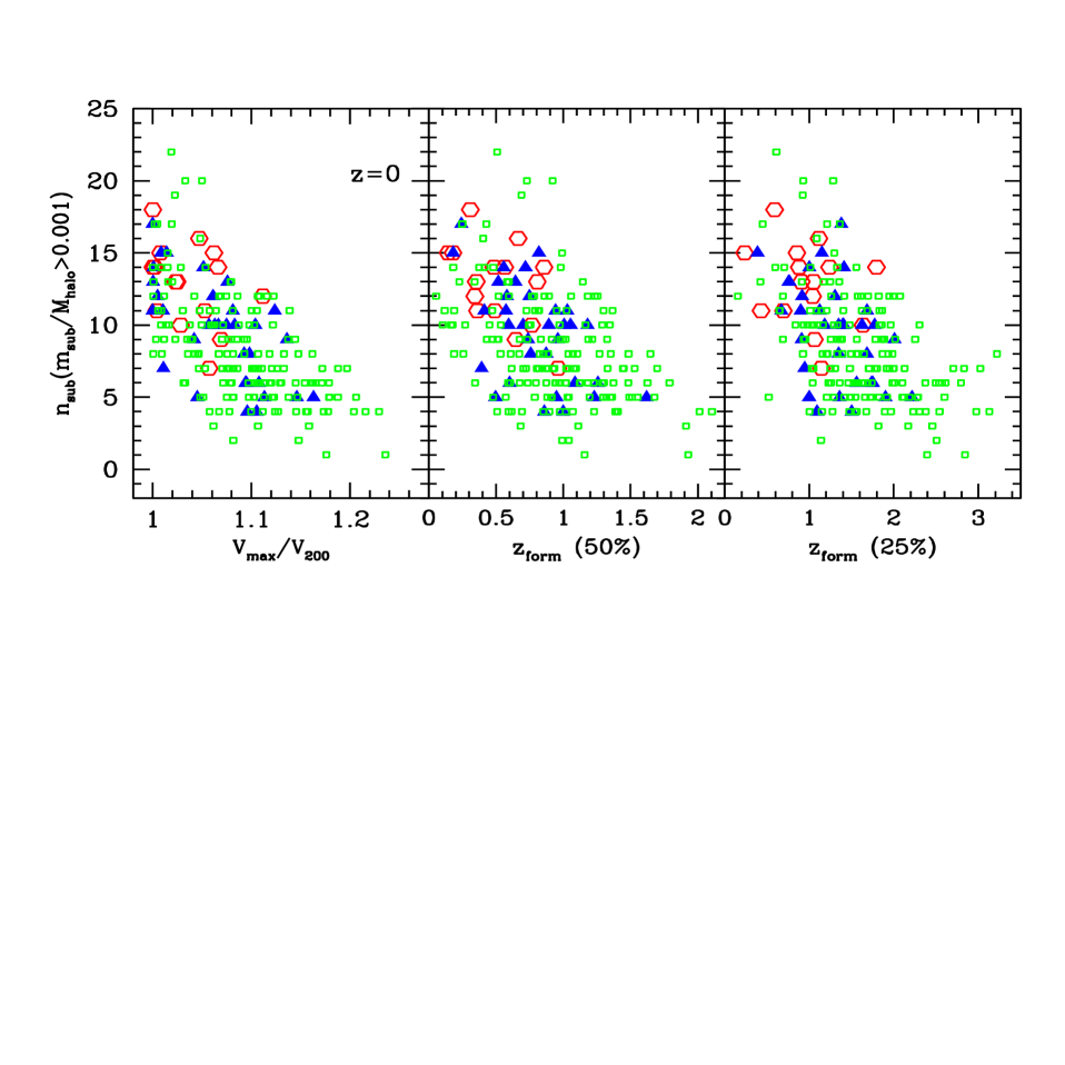
Figure 8: The relation between subhalo abundance and the concentration and the formation redshift of haloes. The left-hand panel shows the number of subhaloes as a function of halo concentration, as measured by $V_{\rm max}/V_{200}$, for our GIF2 and cluster simulations. Only subhaloes containing more than 0.1 per cent of the mass of their parent are considered in compiling these statistics. The middle and right-hand panels show the same measure of subhalo abundance as a function of halo formation times defined as the redshifts when the most massive progenitor has 50 per cent and 25 per cent of the final mass respectively. Open hexagons are for halos in the mass range $3\times 10^{14}h^{-1}{\rm M_{\odot}}<M_{\rm halo}<10^{15}h^{-1}{\rm M_{\odot}}$; filled triangles are for halos with $10^{14}h^{-1}{\rm M_{\odot}}<M_{\rm halo}<3\times 10^{14}h^{-1}{\rm M_{\odot}}$; and open squares are for haloes with $3\times 10^{13}h^{-1}{\rm M_{\odot}}<M_{\rm halo}<10^{14}h^{-1}{\rm M_{\odot}}$.

The total fraction of a halo’s mass invested in subhaloes is an interesting quantity but one for which there is little agreement among the numbers reported in the literature (see, for example, Ghigna et al. 1998, 2000; Springel et al. 2001; Stoehr et al. 2003). Most authors estimate mass fractions between 5 per cent and 20 per cent, but Moore et al.(2001) argue that the true fraction might approach unity if subhaloes could be identified down to extremely small masses. Fig. 7 shows the average mass fraction (within $r_{200}$) in subhaloes more massive than given $m_{sub}$ for GIF2 and cluster haloes in our three ranges of halo mass. These curves show clear trends which can already be inferred from Fig. 5. The subhalo mass fractions appear to converge to well-defined values as the lower limit on subhalo mass is reduced, and the asymptotic value is larger for high-mass than for low-mass haloes. Convergence is a result of the effective slope of the differential abundance function being larger than $-2$, while the trend with halo mass results from the apparent universality of the abundance function at low masses (when normalized by halo mass) together with a dependence of the high-mass cut-off on halo mass.

The masses of individual subhaloes, and so the value of this asymptotic mass fraction, will depend systematically on the algorithm used to define the subhaloes. A variety of different subhalo identification schemes have been used in published studies and undoubtedly account in part for the wide range of subhalo mass fractions quoted. Notice also that since most of the subhalo mass is in the biggest objects, there is a large halo-to-halo variation (well over a factor of 2) in the overall subhalo mass fraction. We show this scatter through the error bars on selected points in the curve for the most massive haloes in Fig. 7. These give the rms scatter of the individual values for the 15 clusters averaged together to make this curve.

4.4 Dependence of subhalo populations on halo concentration and formation time

As demonstrated in Fig. 5, subhaloes tend to be more abundant in more massive haloes. In this section, we show that strong trends are also apparent with halo concentration and with halo formation time. Such systematics are not surprising since Navarro, Frenk & White (1996, 1997) showed that more massive haloes form later and have lower concentrations. They demonstrated that the density profiles of CDM haloes are well described by a simple fitting function with two parameters, $\rho_{s}$ and $r_{s}$. Here $r_{s}$ is a characteristic radius where the logarithmic density profile slope is $-2$, and $\rho_{s}$ is the mass density at $r_{s}$. They also showed that these two quantities are strongly correlated, implying a relation between concentration parameter $c=r_{200}/r_{s}$ and halo mass. More massive haloes are less concentrated. They argued that this is because more massive haloes typically form later. They also showed that at given mass, haloes which form earlier have higher concentrations, a result which has been confirmed by subsequent studies (Wechsler et al. 2000; Bullock et al. 2001; Zhao et al. 2003a, 2003b). This suggests that haloes of similar concentration or formation time should have similar formation histories and so similar numbers of subhaloes.

In the left-hand panel of Fig. 8 we show the number of subhaloes as a function of the concentration of the host, as measured by $V_{\rm max}/V_{200}$. (Using this measure of halo concentration avoids fitting a model to our numerical data). For this comparison, we count only subhaloes with $m_{\rm sub}/M_{\rm halo}>0.001$. This ensures that our results are free of resolution effects. We include data for our GIF2 haloes and for our 8 cluster simulations. Haloes of different mass are plotted using different symbols. Clearly, there is a trend for more concentrated clusters to contain fewer subhaloes and this trend is present and is similar in all three mass ranges.

The middle panel of Fig. 8 shows subhalo abundance as a function of halo formation redshift, defined here as the redshift at which the most massive progenitor of a $z=0$ halo first exceeds half the mass of the final object. We obtain this value by linear interpolation between the redshifts at which we have stored values of the progenitor masses. In this plot also there is a clear trend. Haloes which form late tend to have more subhaloes than haloes which form early, and the relation between substructure and formation time is similar for haloes of different mass. Notice that some haloes form at low redshift yet still contain few subhaloes. Examination of some specific cases suggests that these are products of recent mergers between isolated, similar mass haloes which had previously eliminated much of their substructure. In order to avoid such cases, the right-hand panel of Fig. 8 plots subhalo abundance against a formation time defined as the redshift when the most massive progenitor has 25 per cent of the final mass. The number of recently formed objects with little substructure is reduced and the relation between substructure and formation time appears cleaner.

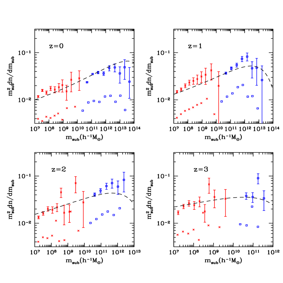
Figure 9: The differential abundance of subhaloes per unit parent halo mass in the GA3n simulation and in our eight cluster simulations is compared with the Sheth & Tormen (1999) formula for the abundance of haloes per unit mass in the Universe as a whole. The four panels refer to four different redshifts as shown. The simulation results are plotted twice in each panel. The symbols without error bars are for subhalo masses as returned by SUBFIND. The points with error bars are obtained when these masses are corrected upwards by a factor of two (see text). The crosses are for GA3n halo; and the squares are the averaged value of $8$ clusters

A final point to note from Fig. 8 is the scatter in the number of subhaloes within objects of given concentration or formation time. The values span a range of up to a factor of four, and the scatter is at most weakly related to halo mass. Clearly the variety of possible formation paths for haloes of given global properties is large enough to produce widely different subhalo populations even among rather similar objects.

4.5 The evolution of the subhalo mass function

Our analysis so far has concentrated on the subhalo distribution within our simulated haloes at redshift $z=0$. Although this is the time when our simulations have the best effective resolution and so can give information over the widest range of scales, it is nevertheless interesting to look at other redshifts in order to investigate the evolution of subhalo properties. Given the near universality we found above, it seems natural to concentrate on the variation with redshift of the abundance of subhaloes per unit parent halo mass, and to compare this with the abundance of haloes per unit mass in the Universe as a whole. This comparison is made in Fig. 9 using the abundance of subhaloes in the most massive progenitor of our ‘Milky Way’ halo in GA3n, and of the main cluster in each of our eight cluster simulations. For these plots we multiply the differential abundance distributions by the square of the (sub)halo mass in order to remove the dominant variation. We can then plot results corresponding to a range of fourteen orders of magnitude in abundance and seven orders of magnitude in (sub)halo mass. The simulation results are shown twice in these plots, for reasons discussed below. The halo abundance predicted for the Universe as a whole by the Sheth & Tormen (1999) mass function is shown by a dashed line in each panel.

Fig. 9 shows that subhalo abundance distributions vary rather little with redshift (see also Kravtsov et al. 2004a). At all redshifts we find the result already noted above for $z=0$. Normalised to total available mass, the subhalo abundance within haloes is very similar to the halo abundance in the Universe as a whole. The offset between the two (the points without error bars and the dashed lines in Fig. 9) is almost independent of mass and epoch and is roughly a factor of four in abundance at fixed mass, corresponding to a factor of two in mass at fixed abundance. This offset can be ascribed to the different ways in which we define the limits of haloes and of subhaloes. Our haloes are bounded by a surface within which the mean interior density is 200 times the critical value, while our subhaloes are bounded by the surface where their density drops to the local value in their host. If the internal density profiles of subhaloes were exactly similar to those of their hosts, and their radial distribution within their hosts exactly paralleled that of the dark matter, then it is easy to see that this difference in boundary definition would cause the masses of subhaloes to be about a factor of two smaller, on average than those of ‘field’ haloes of identical structure. The set of points with error bars in Fig. 9 shows our simulation results when the subhalo masses returned by SUBFIND are doubled to ‘correct’ for this effect. The agreement with the Sheth-Tormen curves is then remarkably good.

We note that the density profiles of the small haloes which give rise to subhaloes are more concentrated than those of the larger haloes they fall into. In addition, we show in the next section that the radial distribution of subhaloes is less concentrated than that of the mass. Both these effects should reduce the difference between the mass assigned to an isolated halo and that assigned to the subhalo it turns into. On the other hand, dynamical processes strip material from a halo once it is incorporated into a larger system, thereby reducing its mass. As we demonstrate in Section 5, most subhaloes fell into their host relatively recently and the amount of stripping is typically quite modest. The combined effect of all these factors is that once subhalo masses are doubled, as above, the number of subhaloes per unit mass within a halo is very similar to the number of small haloes per unit mass in the surrounding universe and thus in the material from which the main halo formed.

4.6 The spatial distribution of subhaloes

How are subhaloes distributed within their parent halo? Superficially, this appears closely related to the distribution of galaxies within clusters, but in fact this relation is complicated because subhalo masses are much more strongly affected by tidal stripping than are the luminosities of the galaxies they contain. As a result the effective total mass-to-light ratio of cluster galaxies is a strongly increasing function of clustercentric radius (see Fig. 12 of SWTK).

It is also interesting to ask whether the radial distribution of subhaloes depends on subhalo mass or on the mass of the parent halo. We address the latter dependence using haloes from our GIF2 and cluster simulations split into the three mass ranges already analysed in Section 4.2. For each mass range we compute the mean fraction by number of all subhaloes within $r_{200}$ that lie within normalized radius $r/r_{200}$. These subhalo number density profiles are shown in the upper left-hand panel of Fig. 10 and are compared with a similarly defined profile for the total mass. All data are shown for $z=0$ and for subhaloes with $m_{\rm sub}/M_{\rm halo}>0.001$ only. We can then get comparable and reliable results for all three halo mass ranges. It is clear that the radial distribution of subhaloes is substantially less concentrated than that of the mass as a whole. There is no significant dependence detected on parent halo mass over the one order of magnitude range tested in this panel, but a weak dependence does appear when we compare with our ‘Milky Way’ simulation GA3n (see below).

Figure 10: Cumulative radial distributions at $z=0$ for subhaloes within $r_{200}$ in various sets of haloes in our simulations. The top left-hand panel shows the fraction of all subhaloes with mass exceeding 0.1 per cent of their host halo mass and lying within $r/r_{200}$ of halo centre. Results are plotted for haloes from our GIF2 and cluster simulations in each of the three mass ranges discussed above. The top right-hand panel shows similar profiles but for various subhalo samples of the 15 massive haloes ($M_{\rm halo}>3\times 10^{14}h^{-1}{\rm M_{\odot}}$) in our GIF2 and cluster simulations. For comparison, we plot cumulative profiles for the total halo mass in both panels. The bottom left-hand panel shows profiles for all subhaloes more massive than $5.78\times 10^{8}h^{-1}{\rm M_{\odot}}$ for two resimulations of a ‘Milky Way’ halo with mass resolution differing by a factor of 10. This mass limit corresponds to 30 particles in the lower resolution simulation. The dotted line shows the profile for subhaloes containing at least 30 particles in the higher resolution simulation. The bottom right-hand panel gives subhalo profiles in these same two simulations but for the subhalo mass range corresponding to 10 to 30 particles in the lower resolution simulation.

Figure 11: Cumulative radial distributions at $z=0$ for subhaloes within $r_{200}$ for the GA3n halo and out 15 clusters. The lines overlying the symbols are the corresponding fits given by Equation (3)

We address the issue of possible dependences on subhalo mass using our cluster resimulations together with the haloes in the most massive bin of our GIF2 simulation (for a total of 15 systems). In the upper right-hand panel of Fig. 10 we show radial number fraction plots for subhalo populations limited above $10^{-3}$ and $10^{-4}$ of the parent halo mass. There appears to be a slight tendency for the more massive haloes to be more centrally concentrated, but the effect is small and it is unclear if it is significant given the relatively small number of parent haloes in our sample.

For these same 15 clusters, the upper right-hand panel of Fig. 10 also shows the cumulative radial profile of subhaloes for which $V_{\rm max}$ is greater than 10 per cent of the parent halo’s value of $V_{200}$. It is interesting that this population appears to be significantly more concentrated than populations defined in these same haloes above a mass threshold. This presumably results from a combination of two effects. A subhalo of given density structure is assigned smaller and smaller masses but largely unchanging $V_{\rm max}$ values as it gets closer to the centre of its parent halo. In addition, subhaloes near the centre of their parent tend to be more heavily affected by tidal stripping than more distant objects. As demonstrated in Section 5.4, such tidal stripping affects the masses of subhaloes more strongly than their maximum circular velocities (Ghigna et al. 2000; Hayashi et al. 2003; Kravtsov et al. 2004b).

The lower panels of Fig. 10 use our ‘Milky Way’ simulations to extend these results to parent haloes of lower mass and to test further for resolution effects. The dashed and solid curves compare the cumulative profiles for subhaloes with mass greater than $5.78\times 10^{7}h^{-1}{\rm M_{\odot}}$ in GA2 and GA3n. This mass corresponds to 30 particles in GA2 and is $M_{\rm halo}/40000$. The two profiles agree extremely well, suggesting that resolution is not seriously effecting our subhalo distributions. Reducing the lower limit on subhalo particle number still further does lead to noticeable effects, as we show in the lower right-hand panel of Fig. 10. Here the comparison is repeated for the subhalo mass range corresponding to 10 to 30 particles in GA2. The abundance of subhaloes is significantly depressed in the lower resolution simulation, particularly in the inner regions. Near the resolution limit of a simulation subhaloes begin to be lost and they disappear preferentially in the inner regions of haloes.

Note that the GA3n result in this panel agrees well with that in the left-hand panel, as does the additional GA3n profile plotted there for subhaloes with more than 30 particles (and so with $m_{\rm sub}>3\times 10^{-6}M_{\rm halo}$). Although all these profiles are close to those plotted in the upper panels for mass-limited subhalo populations within haloes of much higher mass, they are nevertheless noticeably more concentrated. This can be seen in Fig. 11, where we overplot the 30 particle limited subhalo number profile of GA3n and the mean profile for subhaloes with $m_{\rm sub}>10^{-4}M_{\rm halo}$ in our 15 clusters; the subhalo profiles are plotted with symbols. This suggests that as the density profile of the parent halo becomes more concentrated, so too does that of the subhalo population. Note however, that the effect is much weaker for the subhaloes than for the mass as a whole. Our subhalo number density profiles are well fit by the following form:

$$n(<x)/N=(1+ac)x^{\beta}/(1+acx^{\alpha})$$ (3)

where, $x$ is the distance to the host centre in units of $r_{200}$, $n(x$) is the number of subhaloes within $x$, $N$ is the total number of subhaloes inside $r_{200}$, $a=0.244$, $\alpha=2$, $\beta=2.75$, and $c=r_{s}/r_{200}$ is the concentration of the host halo. The lines in Fig. 11 show the predications of this formula for GA3n and for our 15 cluster haloes. Clearly, our fitting formula works quite well. We caution that the concentration dependence here is based on our GA-series simulations only and so should be confirmed with similar resolution simulations of other objects. We emphasize that this formula applies to subhalo populations defined above a given lower mass limit, not to populations defined above circular velocity or luminosity limits.

Our subhalo number density profiles agree well with those presented by Diemand et al. (2003) who also found little dependence either on the mass of the parent or on the mass of the subhalo. They also agree with the subhalo profiles found by De Lucia et al. (2004) for their more massive haloes, but not with the more concentrated profiles found by these authors for their least massive haloes. The differences are relatively small but appear significant. In addition, De Lucia et al. (2004) found massive subhaloes in their simulations to be significantly less centrally concentrated than low-mass subhaloes. At present, we have no clear explanation for this difference with our results. We note that the discrepant results in De Lucia et al are based on a simulation (denoted M3 by them) which was carried out with an early version of GADGET and for which we have other indications that the chosen integration parameters produced overly condensed halo cores and thus, perhaps, overly robust subhaloes (Power et al. 2003). The profiles presented by Gill, Knebe & Gibson (2004) are also similar to ours but are somewhat steeper in the innermost regions. This is likely to reflect the rather different way in which they find subhaloes and define their masses.

Figure 12: The distribution of subhalo accretion times in our simulations. The accretion time is defined as the redshift when the main progenitor first fell into a larger system and so first became a subhalo. The left-hand panels give the fraction by number of present-day subhaloes which were accreted before redshift $z$, while the right-hand panels give the corresponding fractions by mass. Our different mass halo samples are labelled. The upper panels refer to our samples of group and cluster haloes, while the lower panels refer to three simulations of a ‘Milky Way’ halo with differing mass resolution.

5 The evolution of subhaloes

In this section we analyse the evolution of subhaloes by following the history of individual objects. We construct these histories according to the definitions of SWTK. Any particular subhalo identified in one of our stored outputs can have progenitors in the immediately preceding output which are either subhaloes or independent FOF haloes. A subhalo at the earlier time is considered a progenitor if more than half its most-bound particles end up in the subhalo under consideration. A FOF halo is considered a progenitor if it contains more than half the subhalo’s particles. The main progenitor of a subhalo is its largest mass progenitor. By tracing back its main progenitor, the history of any particular subhalo can be followed to the moment of ‘accretion’ when its principal halo ancestor fell onto a larger system and first became a subhalo.

5.1 The history of present subhaloes

It is interesting to know when current subhaloes were typically accreted onto the halo in which they are found. The various panels of Fig. 12 show, for our different parent halo samples, the fractions by number (left) and by mass (right) of present-day subhaloes which were accreted before redshift $z$, as given in the abscissa. In constructing these plots we have considered all subhaloes containing at least 10 particles at $z=0$. The group and cluster mass haloes are shown in the upper panels, and the three simulations of a ‘Milky Way’ halo are shown in the lower panels. It is remarkable that very few of the subhaloes identified at $z=0$ have survived as subhaloes since early times, in agreement with semi-analytical modelling of Zentner & Bullock (2003). Only about 10 per cent of them were accreted earlier than redshift 1 and 70 per cent were accreted at $z<0.5$. These numbers are similar for haloes of all mass and do not depend significantly on the mass of the subhaloes considered. (The apparently discrepant behaviour of the mass fraction for the GA series is just a consequence of focussing on a single realisation in which a relatively massive object happened to accrete at $z\sim 0.7$.) It is clear that subhaloes are typically recent additions to the haloes in which they are seen, substantially more recent, in fact, than typical dark matter particles.

Figure 13: Mean retained mass fractions for subhaloes identified at $z=0$ as a function of the redshift at which they were accreted. Different curves refer to parent haloes of different mass and all present-day subhaloes more massive than $1.73\times 10^{10}h^{-1}{\rm M_{\odot}}$ were included when taking the averages.

Figure 14: The fate of haloes which merge into the main cluster progenitor at redshifts of 2 & 1. Results are shown averaged over our eight cluster simulations in top and bottom panels, respectively. Filled symbols and solid lines show the fraction of haloes which survive as independent subhaloes at each later redshift $z$, while open symbols and dashed lines show the fraction of the total progenitor halo mass attached to these survivors. For each accretion redshift we show results for progenitor haloes containing at least 100 and at least 300 particles. A surviving subhalo is required to have at least 10 particles assigned to it by our subhalo-finder.

5.2 Mass loss from subhaloes as a function of time

When a virialised halo falls onto a bigger structure it loses mass continually through tidal stripping and its orbit slowly decays towards the centre of its new parent as a result of dynamical friction. It is reasonable to expect that subhaloes which fell in earlier should have lost a larger fraction of their original mass by the present day. To measure this mass loss, we calculate the ratio of the mass of each subhalo at $z=0$ to the mass of its progenitor halo just before it was accreted. In Fig. 12 we plot the mean of this ratio for all present-day subhaloes more massive than $1.73\times 10^{10}h^{-1}{\rm M_{\odot}}$ as a function of their accretion redshift, showing results separately for parent haloes of different mass and including haloes from our GIF2 and cluster simulations. The noise at high redshifts in this plot is due to poor statistics. As we saw already in the last section, very few present-day subhaloes were accreted at such early times.

It is clear from Fig. 13 that there is little dependence of mass loss on parent halo mass and that the mean retained mass fraction for surviving subhaloes is a strong function of accretion redshift. Notice that since we compile statistics for subhaloes identified at $z=0$, we neglect objects which have been stripped to masses below our resolution limit or disrupted entirely. As we show in the next section, the retained mass fractions of Fig. 12 are thus substantially higher than those of typical haloes accreted at each redshift.

5.3 The fate of accreted haloes

In this section we follow all the haloes which are accreted onto the main progenitor of a final halo (and so first become subhaloes of it) at redshifts 2 and 1. We are interested to learn what fraction of these survive until $z=0$, what are the final masses of the survivors, what happens to those that do not survive, and how these various fates depend on the mass of the halo which is accreted. Here we use our eight rich cluster simulations to investigate these issues. We begin by finding all progenitors of a final cluster which are independent FOF haloes in the stored output immediately beyond $z=1$ (or 2) but are already listed as part of the main progenitor in the subsequent output. We then attempt to trace all these subhaloes forward until either we reach $z=0$ or they are lost. Three different fates are possible for each accreted halo:

(1)

If it can be followed as a subhalo to $z=0$, we say it survives;

(2)

If it dissolves and becomes part of the main body of its host, we say it disrupts;

(3)

If it merges with a larger subhalo and then loses its identity, we say it merges. We find that no more than a few percent of accreted haloes suffer this fate.

In Fig. 14 we show the fraction of accreted haloes which are identified as surviving at each later redshift, as well as the fraction of the total mass initially assigned to these haloes which remains attached to the surviving subhaloes. We see that while more than 90 per cent of accreted haloes are identified as subhaloes in the output immediately after their accretion, the total subhalo mass is, however, only about half of that assigned to the original haloes. This is a result of the effect already noted above. The algorithm which we use to identify subhaloes bounds them at a substantially higher density than that used to bound isolated haloes. Consequently, if a field halo falls onto a larger system its assigned mass decreases by a factor of two, on average, even if its structure is unchanged. As subhaloes orbit within their parent haloes, their masses are further reduced by tidal stripping. Thus the fraction of the initial mass attached to the survivors continually decreases, and more and more subhaloes drop below the mass limit for identifying them in our simulations.

Fig. 14 gives results for two sets of progenitor haloes at each accretion redshift. These are defined to contain at least 100 and at least 300 particles, corresponding to halo masses exceeding $5\times 10^{9}h^{-1}{\rm M_{\odot}}$ and $1.5\times 10^{10}h^{-1}{\rm M_{\odot}}$, respectively. As can be seen, the mass fraction in the survivors is independent of this mass limit and is 8 per cent for haloes accreted at $z=1$ and 2 per cent for haloes accreted at $z=2$. The fraction of survivors by number does depend on the mass limit. Our samples only contain subhaloes identified with more than 10 particles, so descendents begin to be lost from the lower mass halo sample for mass reduction factors greater than 10 whereas factors exceeding 30 are needed to remove objects from the higher mass sample.

Figure 15: Radial dependence of the accretion redshift (left-hand panel) and retained mass fraction (right-hand panel) for subhaloes of the 15 haloes more massive than $3\times 10^{14}h^{-1}{\rm M_{\odot}}$ in our GIF2 and cluster simulations. In each panel thick solid lines give the mean at each value of $r/r_{200}$ while thin solid lines give the median. The top panels are for subhaloes more massive than $2\times 10^{10}h^{-1}{\rm M_{\odot}}$ while bottom are for subhaloes more massive than $6\times 10^{10}h^{-1}{\rm M_{\odot}}$.

5.4 Radial dependence of accretion time and mass loss

Subhaloes which were accreted onto their parent halo’s main progenitor at early times initially had relatively short orbital periods and so should be located, on average, in the inner regions of the final halo. In addition, a subhalo which has been orbiting within its parent for a long time will have suffered substantially from the effects of dynamical friction and tidal stripping, so its orbit will have decayed by a larger factor than that of a recently accreted subhalo of similar current mass. Both these effects are expected to lead to a correlation between the radial position of a subhalo and its accretion redshift.

In Fig. 15 we plot mean and median values of accretion redshift and of retained mass fraction against $r/r_{200}$ for subhaloes of the 15 haloes in our GIF2 and cluster simulations with masses exceeding $3\times 10^{14}h^{-1}{\rm M_{\odot}}$. The upper and l ower panel refer to subhaloes more massive than $2\times 10^{10}h^{-1}{\rm M_{\odot}}$ and more massive than $6\times 10^{10}h^{-1}{\rm M_{\odot}}$ respectively. Clearly there is indeed a strong age-radius relation which is similar for subhaloes of differing mass. Recently accreted subhaloes tend to occupy the outer regions of their host, while older subhaloes reside preferentially in the inner regions. In addition, haloes near the centre typically retain a much smaller fraction of their progenitor halo’s mass than those in the outer regions (The reasons for this are discussed in some detail by Kravtsov et al. (2004b)). The large difference between the median and the mean in the accretion redshift plot is a reflection of the substantial skewness of the distribution. As we already saw in Fig. 12 and 13, tidal stripping is clearly very effective and, as a consequence, the ancestors of inner subhaloes were more massive than those of outer subhaloes of the same mass. Thus in a galaxy cluster inner subhaloes are likely to host brighter galaxies than outer subhaloes of similar mass.

6 Summary and discussion

We have used a single, large-scale cosmological simulation together with two sets of resimulations of the formation of individual cluster and galaxy haloes to carry out a systematic study of the properties of dark halo substructure in the concordance $\Lambda$CDM universe. In agreement with the earlier work of Jenkins et al. (2001), Reed et al. (2003) and Yahagi et al. (2004) we find the abundance of haloes (defined using a friends-of-friends group finder with linking length $b=0.2$) to be well described by the Sheth & Tormen (1999) mass function down to masses of a few times $10^{10}{\rm M_{\odot}}$ and out to a redshift of 5. Our main results for the subhalo populations within these haloes can be summarized as follows:

(1)

The subhalo populations of different haloes are not simply scaled copies of each other, but vary systematically with global halo properties. On average, massive haloes contain more subhaloes above any given fraction of parent mass than do lower mass haloes, and these subhaloes contain a larger fraction of the parent’s mass. At given halo mass, subhaloes are more abundant in haloes which are less concentrated, or formed more recently.

(2)

There is considerable scatter in the abundance of subhaloes between haloes of similar mass, concentration or formation time. This presumably reflects differences in the details of halo assembly.

(3)

For subhalo masses well below that of the parent halo the mean subhalo abundance per unit parent mass is independent of the actual mass of the parent. It is very similar to the abundance of haloes per unit mass in the universe as a whole, once a correction is made for the differing bounding density within which the masses of haloes and subhaloes are defined.

(4)

Normalised in this way to total parent halo mass, the mean abundance of subhaloes as a function of maximum circular velocity is also quite similar to the abundance per unit mass of haloes as a function of $V_{\rm max}$. For subhaloes the abundance per unit mass is about a factor of two lower at given $V_{\rm max}$ than for haloes. Equivalently, the $V_{\rm max}$ values of subhaloes at given abundance per unit mass are about 25 per cent lower than those for haloes.

(5)

In agreement with previous studies, we find the the radial distribution of subhaloes within their parent haloes to be much less concentrated than that of the dark matter. We find no significant dependence of this radial profile on the mass of the subhaloes and only a very weak dependence on the mass (or concentration) of the parent halo. To a good approximation the radial distribution of subhaloes appears ‘universal’ and we give a fitting formula for it in equation 3.

(6)

The subhalo number density profile does depend on how the population is defined. Subhalo populations defined above a minimum circular velocity limit are significantly more concentrated than those defined above a minimum mass limit.

(7)

Most subhaloes in present-day haloes fell into their parent systems very recently. Only about 10 per cent of them were accreted earlier than $z=1$ and 70 per cent were accreted at $z<0.5$. These fractions depend very little on the mass of the subhaloes or on that of their parents

(8)

The rate at which tidal effects reduce the mass of subhaloes is not strongly dependent on the mass of the accreted object or on that of the halo it falls into. About 92 per cent of the total mass of haloes accreted at $z=1$ is removed to become part of the ‘smooth’ halo component by $z=0$. For haloes which fall in at $z=2$ this fraction is about 98 per cent. Note that the highest mass accreted objects merge into the central regions more quickly because of dynamical friction effects.

(9)

Subhaloes seen near the centre of their parent haloes typically fell in earlier and retain a smaller fraction of their original mass than subhaloes seen near the edge. Thus inner subhaloes may be expected to host brighter galaxies than outer subhaloes of similar mass (see Springel et al. 2001).

These properties suggest a relatively simple picture for the evolution of subhalo populations. A substantial fraction of the mass of most haloes has been added at relatively recent redshifts, and this mass is accreted in clumpy form with a halo mass distribution similar to that of the Universe as a whole. Since tidal stripping rapidly reduces the mass of subhaloes, the population at any given mass is dominated by objects which fell in recently and so had lower mass (and thus more abundant) progenitors. The orbits of recently accreted objects spend most of their time in the outer halo, so that subhaloes of given mass are substantially less centrally concentrated than the dark matter as a whole. Subhaloes which are seen near halo centre have shorter period orbits and so must have fallen in earlier. They thus retain a relatively small fraction of their initial mass.

Comparison of these subhalo properties with observation is far from simple. The recent accretion of most subhaloes means that the galaxies at their centres were almost fully formed by the time they became part of their current host. We might therefore expect their observable properties to be more closely related to the mass of their progenitor haloes and to their accretion redshifts than to the current masses of their subhaloes. Explicit tracking of galaxy formation during the assembly of cluster haloes shows that these differences can be large. For example, both Diaferio et al. (2001) and Springel et al. (2001) find radial number density profiles for magnitude limited samples of galaxies which are similar both to the underlying dark matter profiles and to the observed profiles of real clusters, but which are very different from the number density profiles for mass limited subhalo samples. Similar differences are to be expected between the velocity biases of galaxies and subhaloes. Models for the stellar content of subhaloes which are based purely on their current mass and internal structure are very unlikely to be successful. The past history of subhaloes must be included to get realistic results, as must galaxies associated with apparently disrupted subhaloes. We investigate these issues further in a companion paper (Gao et al. 2004b);

References

- [1] Bullock J. S., Kolatt T. S., Sigard Y., Sommervile R. S., Kravtsov A. V., Klypin A. A, Primack J. R., Dekel A., 2001, 321, 559
- [2] Couchman H. M. P., Pearce F. R., Thomas P. A., ApJ, 1995, 452, 797
- [3] Davis M., Efstathiou G., Frenk C. S., White S. D. M., 1985, MNRAS, 292, 371
- [4] De Lucia G., Kauffmann G., Springel V., White S. D. M, Lanzoni B., Stoehr F., Tormen G., Yoshida N., 2003, MNRAS, 348, 333
- [5] Desai V., DAlcanton J. J., Mayer L., Reed D., Quinn T, Governato F., 2004, MNRAS, 351, 265
- [6] Diaferio A., Kauffmann G., Balogh M. L.,White S. D. M.; Schade D., Ellingson E., 2001, MNRAS, 323, 999
- [7] Diemand J., Moore B., Stadel J., 2004, MNRAS, 352, 535
- [8] Efstathiou G., Davis M., White S. D. M., Frenk C. S., 1985, APJS, 57, 241
- [9] Frenk C. S, et al, 1999, ApJ, 525, 554
- [10] Gao L., Loeb A., Peebles P. J. E., White S. D. M., Jenkins A., 2004a, ApJ in press, preprint, astro-ph/0312499
- [11] Gao L., De Lucia G., White S. D. M., Jenkins, A., 2004b, MNRAS, 352, L1
- [12] Ghigna S., Moore B., Governato F., Stadel J., 1998, MNRAS, 300, 146
- [13] Ghigna S., Moore B., Governato F., Lake G., Quinn T., Stadel J., 2000, ApJ, 544, 616
- [14] Gill S. P. D.l, Knebe A., Gibson B. K, 2004, MNRAS, 351, 399
- [15] Hayashi E., Navarro J. F., Taylor, J. E., Stadel J., Quinn, T., 2003, ApJ, 584, 541
- [16] Hayes W. B, 2003, ApJ, 587, L59
- [17] Helmi A., White S. D. M, MNRAS, 323, 529
- [18] Jenkins A., Frenk C.S., Pearce F.R., Thomas P.A., Colberg J.M., White S. D. M., Couchman H. M. P., Yoshida N., 2001, MNRAS, 321, 372
- [19] Klypin A., Kravtsov A., Valenzuela O., Prada F., 1999, ApJ, 522, 82
- [20] Klypin A., Gottloeber, Kravsov A., Khokhlov M., 1999b, ApJ, 516, 530
- [21] Kravtsov A. V., Berlind A. A., Wechsler R. H., Klypin A. A., Gottloeber S., Allgood B., Primack J. R., 2004a, ApJ, 609, 35
- [22] Kravtsov A. V., Gnedin O. Y., Klypin A. A., 2004b, ApJ, 609, 482
- [23] Lacey C., Cole S., 1993, MNRAS, 262, 627
- [24] Lacey C., Cole S., 1994, MNRAS, 271, 676
- [25] Macfarland T., Couchman H. M. P., Pearce F. R., Pichlmeier J., 1998, New Astron., 3, 687
- [26] Mo H. J., White S. D. M., 1996, MNRAS, 283, 347M
- [27] Moore B., Katz N.,Lake G.ApJ,457,455
- [28] Moore B., Ghigna S., Governato F., Lake G., Quinn T., Stadel J., Tozzi P., 1999 ApJ, 524, 19
- [Moore et al.(2001)] Moore, B., Calcáneo-Roldán, C., Stadel, J., Quinn, T., Lake, G., Ghigna, S., & Governato, F. 2001, Phys. Rev. D, 64, 063508
- [29] Navarro J. F., Frenk C. S., White S. D. M., 1997, ApJ, 490, 493
- [30] Navarro J. F., Hayashi E., Power, C., Jenkins, A. R., Frenk, C. S., White, S. D. M., Springel V.; Stadel J., Quinn T. R., 2004, MNRAS, 349, 1039
- [31] Power C., Navarro J. F., Jenkins, A., Frenk, C. S., White S. D. M., Springel V., Stadel J., Quinn T., 2003, MNRAS, 338, 14
- [32] Press W.H., Schechter P., 1974, ApJ, 187, 452
- [33] Reed D., Gardner J., Quinn T., Stadel J., Fardal M., Lake G., Governato F., 2003, MNRAS, 346, 565
- [34] Seljak U., Zaldarriaga M., 1996, ApJ, 469, 437
- [35] Sheth R., Tormen G.,1999, MNRAS, 308,119
- [36] Sheth R., Mo H. J., Tormen G., 2001, MNRAS, 323, 1
- [37] Springel V., Yoshida N., White S. D. M., 2001a, New Ast. 6, 79
- [38] Springel V., White S. D. M., Tormen G., Kauffmann G., 2001b, MNRAS, 328, 726(SWTK)
- [39] Stoehr F., White S. D. M, Tormen G., Springel V.,2002, MNRAS, 335, 762
- [40] Stoehr F., White S. D. M, Springel V., Tormen G., Yoshida N., 2003, MNRAS, 345, 1313
- [41] Wechsler R. H., Bullock J. S., Primack J. R., Kravtsov A. V., Dekel A., 2002, ApJ, 586, 52
- [42] White S. .D. M, 1993, in schaeffer R., Silk J., Spiro M., Zinn-Justin J., eds, Cosmology and large Scale Structure, Les Houches Session LX. Elsevier, Amsterdam, P.77
- [43] White S. D. M, Davis M., Efstathiou G., Frenk C. .S.,1987, Nature, 330, 451
- [44] Yoshida N., Sheth R. K., Diaferio A., 2001, MNRAS, 328, 669
- [45] Yahagi H., Nagashima M., Yoshii Y., 2004, ApJ, 605, 709
- [46] Zentner, Bullock, 2003, ApJ, 598, 49
- [47] Zhao D. H., Mo H. J., Jing Y. P., Boerner G., 2003a, MNRAS, 339, 127
- [48] Zhao D. H., Jing Y. P., Mo H. J., Boerner G., 2003b, ApJ, 597L, 9