Three-dimensional Simulations of Disk Accretion to an Inclined Dipole: II. Hot Spots and Variability

Abstract

The physics of the “hot spots” on stellar surfaces and the associated variability of accreting magnetized rotating stars is investigated for the first time using fully three-dimensional magnetohydrodynamic simulations. The magnetic moment of the star ¯ is inclined relative to its rotation axis $\bf{\Omega}$ by an angle $\Theta$ (we will call this angle the “misalignment angle”) while the disk’s rotation axis is parallel to $\bf{\Omega}$. A sequence of misalignment angles was investigated, between $\Theta=0^{\circ}$ and $90^{\circ}$. Typically at small $\Theta$ the spots are observed to have the shape of a bow which is curved around the magnetic axis, while at largest $\Theta$ the spots have a shape of a bar, crossing the magnetic pole. The physical parameters (density, velocity, temperature, matter and energy fluxes, etc.) increase toward the central regions of the spots, thus the size of the spots is different at different values of these parameters. At relatively low density and temperature, the spots occupy approximately $10-20\%$ of the stellar surface, while at the highest values of these parameters this area may be less than $1\%$ of the area of the star. The size of the spots increases with the accretion rate. The light curves were calculated for different $\Theta$ and inclination angles of the disk $i$. They show a range of variability patterns, including one maximum-per-period curves (at most of angles $\Theta$ and $i$), and two maximum-per-period curves (at large $\Theta$ and $i$). At small $\Theta$, the funnel streams may rotate faster/slower than the star, and this may lead to quasi-periodic variability of the star. The results are of interest for understanding the variability and quasi-variability of Classical T Tauri Stars, millisecond pulsars and cataclysmic variables.

Department of Astronomy, Cornell University, Ithaca, NY 14853-6801;  romanova@astro.cornell.edu

Keldysh Institute of Applied Mathematics, Russian Academy of Sciences, Moscow, Russia;  ustyugg@spp.Keldysh.ru

Institute of Mathematical Modelling, Russian Academy of Sciences, Moscow, Russia; koldoba@spp.Keldysh.ru

Department of Astronomy, Cornell University, Ithaca, NY 14853-6801;  RVL1@cornell.edu

Subject headings: accretion, dipole — plasmas — magnetic fields — stars: magnetic fields — X-rays: stars

Draft version

1 Introduction

In accreting magnetized stars the inflowing matter is channelled to regions near the magnetic poles of the star, forming “hot spots” on the star’s surface (e.g., Ghosh & Lamb 1979; Uchida & Shibata 1985; Camenzind 1990; Königl 1991; Shu et al. 1994; Hartmann et al. 1994). The hot spots form under conditions in which the star’s magnetic field is strong enough to form a magnetosphere. Examples include classical T Tauri stars (e.g., Herbst et al. 1986; Bouvier & Bertout 1989; Johns & Basri 1995; 1998; Petrov, et al. 2001a,b; Alencar & Batalha 2002), cataclysmic variables (e.g., Wickramasinghe, Wu, & Ferrario 1991; Livio & Pringle 1992; Warner 1995; Warner 2000), X-ray pulsars (e.g., Ghosh & Lamb 1979; Trümper et al. 1985; Bildsten et al. 1997) and millisecond pulsars (e.g., Chakrabarty, et al. 2003). These objects have different dimensions and magnetic field strengths, but the underlying physics of the magnetospheric accretion and hot spots’ properties are expected to be similar.

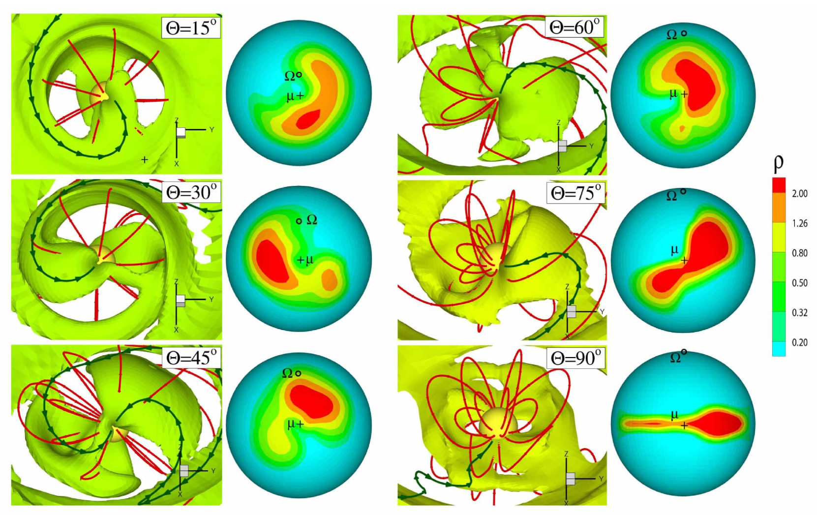
  Fig. 1.—: Matter flow near the star and hot spots for the case of a relatively warm disk ($T_{d}=0.03$). The square panels show the surfaces of the density in the magnetospheric flows (green color corresponds to $\rho=0.3-0.4$, while yellow-green color to $\rho=0.6$). Red lines are sample magnetic field lines; the dark-green lines show the sample streamlines of matter flow. The circular panels show density distribution in the hot spots for different misalignment angles $\Theta$. For $\Theta=15^{\circ},30^{\circ}$ and $45^{\circ}$, the magnetic axis is directed towards the observer, while for $\Theta=60^{\circ},75^{\circ}$ and $90^{\circ}$, it is directed at an angle $45^{\circ}$ relative to the observer. It is shown by the crosses in the circular panels. The direction of the rotation axis is shown with the open circles.

The observed variability/quasi-variability of these objects can be due to a number of possible phenomena in the magnetosphere (see, e.g., Bouvier 2003; Petrov 2003). One of the time-scales may be associated with the hot spots. In spite of the large volume of the observational data on variability of these stars, relatively little is known about the properties of the hot spots.

For example, in classical T Tauri stars (CTTS), hot spots radiation is associated with veiling of the continuum radiation and was analyzed for a number of CTTS. Herbst & Koret (1988) and Bouvier et al. (1986, 1993) estimated parameters of the hot spots assuming a model with black body radiation, while Lamzin (1995), Calvet & Gullbring (1998), Gullbring et al. (2000), and Ardila & Basri (2000) used models of radiation from a shock wave. They concluded that the area of the star covered with the hot spots in different CTTS varies from $0.3\%$ to $20\%$ depending on the accretion rate and other factors. In all models, however, the hot spots were considered to be homogeneous, that is, of the same density and temperature. Further, some of the models did not take into account the effect of limb-darkening. Additionally, the shape and location of the hot spots were not known because they can be derived only from a three-dimensional analysis. Similar problems and questions appear during analysis of X-ray pulsars and cataclysmic variables. Thus, it is important to study the properties of the hot spots in greater detail. For analysis of the hot spots we use results of our previous three-dimensional simulations (Romanova et al. 2003, hereafter - R03), and also perform new simulations at a lower temperature in the disk and at a variety of parameters of the star and the accretion flow.

The main questions which can be answered are: (1) What are the shapes of the hot spots? (2) What is the distribution of physical parameters (density, temperature) in the spots? (3) What is the area covered by the spots at different physical parameters? (4) What are the observed light curves at different misalignment angles $\Theta$ and different inclination angles of the disk $i$?

In §2 of the paper we describe the underlying model and dimensional examples for CTTS and millisecond pulsars. In §3 we discuss the expected physical properties of the hot spots. In §4 we calculate the intensity of radiation from the hot spots and the associated light curves. In §5 we discuss dependence of results on different parameters, limitations of the model and future work. §6 gives the summary of our work.

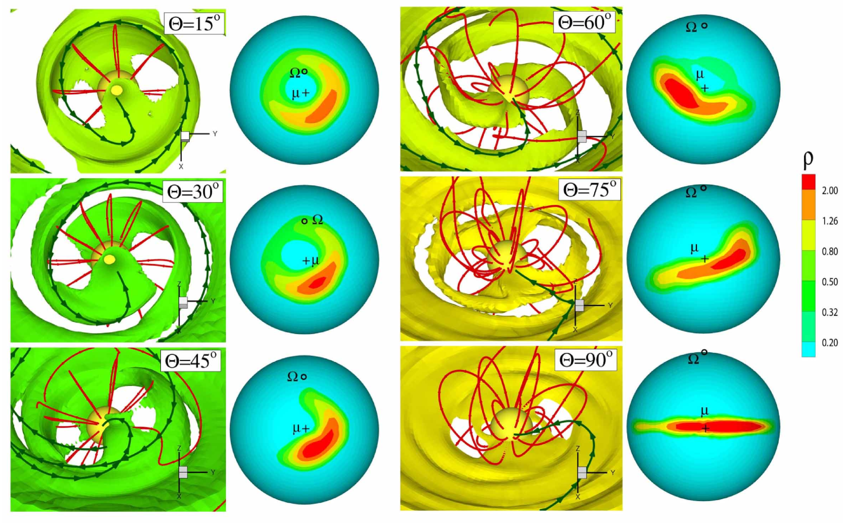
  Fig. 2.—: Same as Figure 1 but for cooler disk ($T_{d}=0.01$).

2 The Model and Reference Values

Below we briefly describe the numerical model of R03, initial and boundary conditions, and reference values for CTTS and millisecond pulsars.

2.1 The Model

Disk accretion to a rotating star with an inclined dipole magnetic field was investigated with three-dimensional MHD simulations. The magnetic moment ¯ of the dipole is inclined to the star’s rotation axis ${\bf\Omega}$ by an angle $\Theta$. The rotation axis of the star coincides with the rotation axis of the disk. The value of the magnetic moment $\mu=|{\hbox{\tenbg\char 22\relax}}|$ is restricted by computer resources. It is difficult to calculate in three dimensions large magnetospheres, where the magnetospheric radius $R_{m}$ is much larger than the star’s radius $R_{*}$. This is because of the strong variation ($\propto 1/R^{3}$) of the dipole magnetic field. In R03, simulations were done for $R_{m}/R_{*}\approx 2-5$. These values are appropriate for many Classical T Tauri Stars (CTTS) and millisecond pulsars. For larger magnetospheres, the inner boundary may be interpreted as an intermediate layer of magnetosphere.

A Godunov-type numerical code was used to solve the full system of ideal MHD equations in three-dimensions space written in a “cubed sphere” coordinate system rotating with the star (Koldoba et al. 2002; R03). We use a reference frame $(X,Y,Z)$ rotating with the star. This frame is oriented such that the $Z$ axis is aligned with the star’s rotation axis and vector ¯ is in the $(X,Z)$ plane.

The quasi-equilibrium initial conditions were proposed and tested in axisymmetric model in Romanova et al. (2002 - hereafter R02) and in three dimensions in R03. These initial conditions take into account initial balance of gravitational, pressure gradient and centrifugal forces. Although this initial condition does not include the magnetic field, it avoids the possible initial discontinuity of the poloidal magnetic field lines at the boundary between the disk and corona (corona above the disk rotates with the angular velocity of the disk). Test simulations with a non-rotating corona show strong magnetic braking and accretion of the disk with a speed close to the free-fall speed (see Hayashi, Shibata & Matsumoto 1996, some runs of Miller and Stone 1997). The new initial conditions decrease this initial magnetic braking dramatically, but not completely. There is a residual small magnetic braking which determines a slow inward accretion of matter to the star. This accretion is used as a source of accreting matter in most of simulations. To check the validity of this approach, we added simplified “alpha” viscosity to the code, where only the largest terms were taken into account (as in R02) and performed a set of simulations at $\Theta=15^{\circ}$ and at a variety of $\alpha$ parameters (see §5.1). Simulations have shown that the velocity of the accretion flow induced by the residual magnetic braking corresponds to viscous flow with $\alpha\approx 0.01-0.02$. These initial conditions allowed us to observe for the first time the magnetospheric funnel flows from the disk to the star in two and three dimensions and to investigate them in detail (see R02, and R03).

We consider the case when the star rotates relatively slowly with angular velocity $\Omega_{*}\approx 0.04\Omega_{K*}$, where $\Omega_{K*}=\sqrt{GM/R_{*}^{3}}$ - is the brake-up angular velocity of the star. For the case of T Tauri stars, this corresponds to a slow rotation rate ($T\approx 9.4~{}{\rm days}$ for the parameters used in R02). This rotation velocity was chosen simply because it was the main case of R03. Test cases with faster rotation of the star were also performed.

We consider two main cases: (1) a relatively hot disk where the flow to the star is subsonic, and (2) a cooler disk, where the flow is supersonic. The important parameters are the initial densities in the disk $\rho_{d}$ and corona $\rho_{c}$, and the initial temperatures in the disk $T_{d}$ and corona $T_{c}$. These values are determined at the fiducial point at the boundary between the disk and corona (at the inner radius of the disk) such that to support pressure balance in vertical direction. In two-dimensional simulations (R02) we used such parameters that: $\rho_{c}=0.01\rho_{d}$, $T_{d}=0.01T_{c}$ and obtained supersonic funnel streams, because the sound speed is relatively low, $c_{s}\approx 0.1v_{K}$. However, in 3D simulations in R03 we were able to cover only a “softer” range of parameters: $\rho_{c}=0.03\rho_{d}$, $T_{d}=0.03T_{c}$, when the disk has higher temperature and $c_{s}\approx 0.17v_{K}$. In this paper we use results of R03 and newer runs with lower temperature in the disk ($c_{s}\approx 0.1v_{K}$).

  Fig. 3.—: Fraction of the star’s surface area ${\it f}$ covered by the hot spots with density larger than $\rho$ for different misalignment angles $\Theta$. The left panel shows the case of warmer disk, $T_{d}=0.03$, while the right panel the case of cooler disk, $T_{d}=0.01$.

The boundary conditions are similar to those in R03. At the stellar surface there are “free” boundary conditions to the density and pressure. The poloidal components of the magnetic field are determined from the fact that the star is treated as a perfect conductor rotating at the rate ${\bf\Omega}=\Omega\hat{\bf z}$. There is however a “free” condition to the azimuthal component of the magnetic field: ${\partial(RB_{\phi})}/{\partial R}=0$ so that magnetic field lines have a “freedom” to bend near the stellar surface. In the reference frame rotating with the star the flow velocity is adjusted such that to be parallel to ${\bf B}$ at $R=R_{*}$. This inner boundary condition is valid when the flow is subsonic. In the supersonic case there will be standoff shock, but it requires separate investigation. From the other side, these boundary conditions are valid for any of these cases if the boundary is not the surface of the star, but corresponds to some intermediate layers of the magnetosphere, while the real surface of the star is at smaller radii. Thus, the obtained parameters of the hot spots reflect the distribution of these parameters in the cross-section of the funnel streams.

At the outer boundary $R=R_{\rm max}$, free boundary conditions are taken for all variables. We investigated different types of boundary conditions for the magnetic field, but did not observe a significant difference, because the magnetic field of the dipole decreases very rapidly with distance and the difference is much less dramatic compared to monopole magnetic field (Ustyugova et al. 1999). We also investigated the possible influence of the outer boundary conditions by running cases where the simulation regions had $R_{\rm max}/R_{*}=14$, $40$, and $194$. We find the same results except for the case $R_{\rm max}/R_{*}=14$ where the accretion rate decreases too fast because the reservoir of matter in the disk is too small. Results for the medium and large regions are very close, so that we took $R_{\rm max}/R_{*}=40$ as a standard size of the simulation region.

2.2 Dimensionless Variables and Reference Values

We use the following dimensionless variables: the length scale $r^{\prime}=r/R_{0}$, the fluid velocity ${\bf v}^{\prime}={\bf v}/v_{0}$, the density $\rho^{\prime}=\rho/\rho_{0}$, the magnetic field $B^{\prime}=B/B_{0}$, the pressure $p^{\prime}=p/p_{0}$, the temperature $T^{\prime}=T/T_{0}$ and time $t^{\prime}=t/t_{0}$. The ‘zero’ subscript variables are dimensional reference values, which are different for different objects.

The reference values are determined as follows: the unit of distance $R_{0}$ is taken to be an initial inner radius of the disk, $R_{0}=(R_{d})_{t=0}$, so that $r^{{}^{\prime}}=1$ at this radius. The star has radius $R_{*}=0.35R_{0}$. The reference velocity is the Keplerian velocity at $R_{0}$, $v_{0}=(GM/R_{0})^{1/2}$, where $\omega_{0}=v_{0}/R_{0}$ is the angular velocity. The reference time is $t_{0}=R_{0}/v_{0}$. However, in discussing our results we measure time in units of the Keplerian period of the disk, $P_{0}=2\pi t_{0}$. The reference magnetic field $B_{0}$ is the initial magnetic field strength at $r=R_{0}$. The reference density is taken to be $\rho_{0}=B_{0}^{2}/v_{0}^{2}$. The reference pressure is $p_{0}=\rho_{0}v_{0}^{2}$. The reference temperature is $T_{0}=p_{0}/{\cal R}\rho=v_{0}^{2}/{\cal R}$, where ${\cal R}$ is the gas constant. The reference accretion rate is $\dot{M}_{0}=\rho_{0}v_{0}R_{0}^{2}$. The reference energy flux is $\dot{E}_{0}=\rho_{0}v_{0}^{3}R_{0}^{2}$. The reference value for the black-body temperature of the hot spots is $(T_{eff})_{0}=(\rho_{0}v_{0}^{3}/\sigma)^{1/4}$, where $\sigma$ is the Stephan-Boltzmann constant.

Subsequently, we drop the primes on the dimensionless variables and show dimensionless values in most of the figures. Two types of initial conditions for the disk in dimensionless variables are considered: $\rho_{d}=1$, $\rho_{c}=0.03$, $T_{d}=0.03$ and $T_{c}=1$ for the warmer disk, and $\rho_{d}=1$, $\rho_{c}=0.01$, $T_{d}=0.01$ and $T_{c}=1$ for the cooler disk. Below we discuss dimensional examples for stars with relatively small magnetospheres, CTTS and millisecond pulsars.

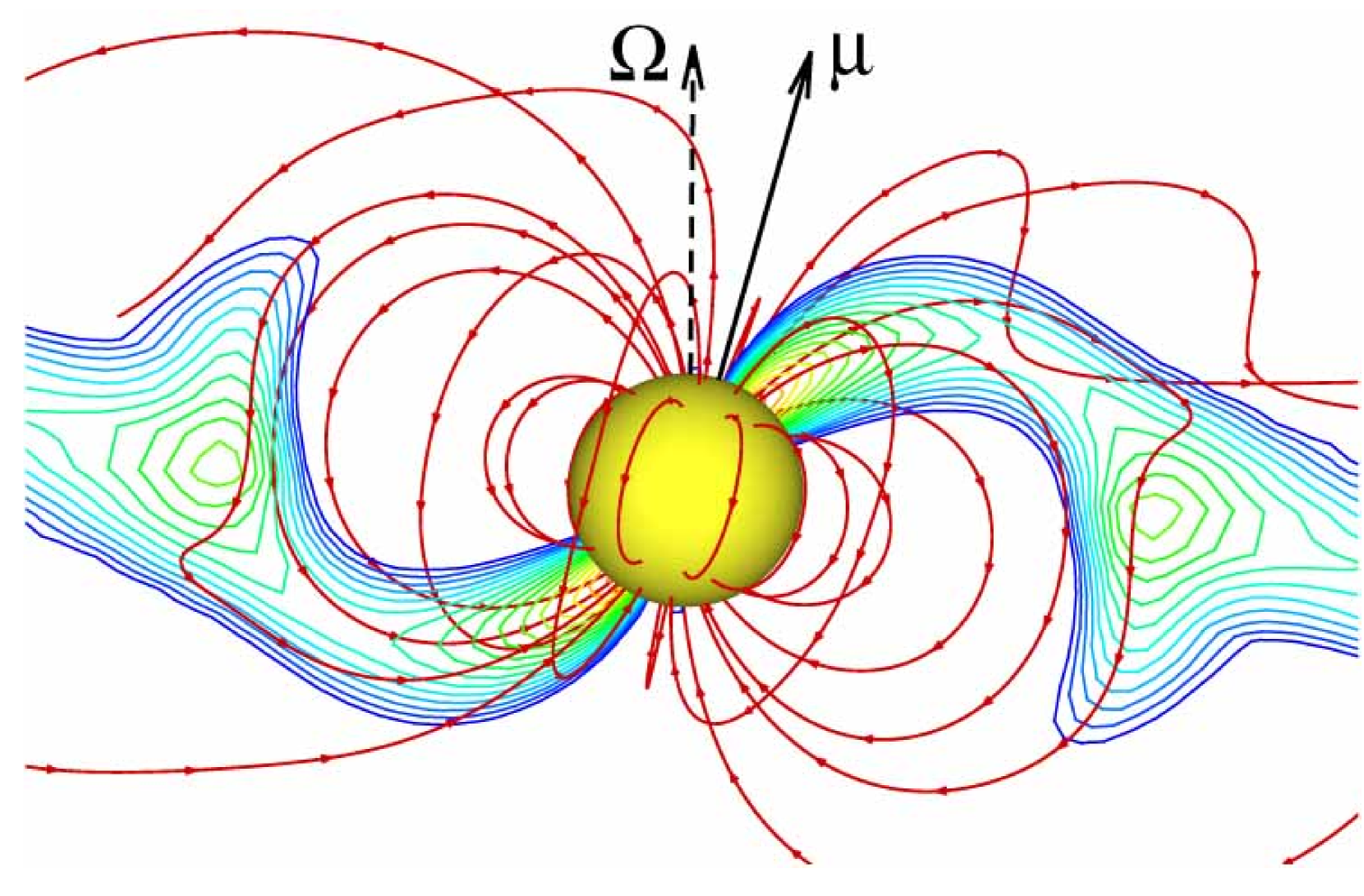
  Fig. 4.—: An $X-Z$ slice through the middle of the funnel stream at $\Theta=15^{\circ}$. The contour lines show the plane cross-section of the density distribution inside the funnel stream. The density changes exponentially from $\rho=0.2$ (blue) to $\rho=2.0$ (red). The density in the corona above the disk is $\rho=0.01-0.02$. Red lines with arrows show selected magnetic field lines. The magnetic moment ¯, and the rotation axis $\bf\Omega$ are shown.

2.3 Reference Values for Classical T Tauri Stars

Here, we discuss the numerical parameters for a typical CTTS. We take the mass of the star to be $M_{*}=0.8M_{\odot}$, and its radius $R_{*}=1.8R_{\odot}$. The magnetic field at the surface of the star is assumed to be $B_{*}=10^{3}~{}{\rm G}$. The reference value of length is $R_{0}=(1/0.35)R_{*}\approx 2.86R_{*}\approx 3.6\times 10^{11}~{}{\rm cm}$. The size of the simulation region corresponds to $R_{\rm max}\approx 40R_{*}\approx 0.34~{}{\rm AU}$. The reference velocity is $v_{0}\approx 1.9\times 10^{7}~{}{\rm cm/s}$. The period of Keplerian rotation of the inner radius of the disk is $P_{0}\approx 1.38~{}{\rm days}$. We consider that the star rotates relatively slowly, $P_{*}=9.4~{}{\rm days}$ which corresponds to many CTTSs. Simulations for higher rotational velocities did not bring principally new results (excluding the propeller stage of course, which we do not discuss here). The reference magnetic field is $B_{0}=B_{*}(R_{*}/R_{0})^{3}\approx 42.7~{}{\rm G}$. The reference density is $\rho_{0}=4.9\times 10^{-12}~{}{\rm g/cm^{3}}$ or $n=3.06\times 10^{12}~{}{\rm cm^{-3}}$ which is typical for T Tauri star disks (see, e.g., Hartmann et al. 1998). The reference temperature is $T_{0}=4.5\times 10^{6}~{}{\rm K}$ which corresponds to typical temperature in the corona and temperature $T_{d}=4.5\times 10^{4}~{}{\rm K}$ in the innermost part of the disk for the run typical for CTTS ($T_{d}=0.01$, $T_{c}=1$). The reference mass accretion rate is $\dot{M}_{0}\approx 1.2\times 10^{19}~{}{{\rm g/s}}\approx 1.9\times 10^{-7}~{}{\rm M_{\odot}}/{\rm year}$. The reference value for the energy flux is $\dot{E}_{0}\approx 4.5\times 10^{33}~{}{\rm ergs/s}$ and for black-body temperature: $(T_{eff})_{0}=5.0\times 10^{3}~{}{\rm K}$. The dimensionless values of the intensity in the Figures 7-9 are $J\approx 2\times 10^{-3}-1.7\times 10^{-2}$ which corresponds to the dimensional values $J\dot{E}_{0}\approx 9.0\times 10^{30}-7.6\times 10^{31}~{}{\rm ergs/s}$.

2.4 Reference Values for Millisecond Pulsars

We take the mass of the neutron star to be $M_{*}=1.4~{}{\rm M_{\odot}}=2.8\times 10^{33}~{}{\rm g}$, its radius $R_{*}=10~{}{\rm km}=10^{6}~{}{\rm cm}$, and the surface magnetic field $B=10^{8}~{}{\rm G}$. The reference length scale is $R_{0}\approx 2.86R_{*}=2.86\times 10^{6}~{}{\rm cm}$. The reference velocity is $v_{0}=8.1\times 10^{9}~{}{\rm cm/s}$. The reference period is $P_{0}=2.2\times 10^{-3}~{}{\rm s}$. In application to millisecond pulsars often the frequency is analyzed. The reference frequency is $\nu_{0}=1/P_{0}\approx 454~{}{\rm Hz}$. The reference magnetic field is $B_{0}=B_{*}(R_{*}/R_{0})^{3}\approx 4.3\times 10^{6}~{}{\rm G}$. The reference density is $\rho_{0}=2.8\times 10^{-7}~{}{\rm g/cm^{3}}$. The reference temperature is $T_{0}=7.8\times 10^{11}~{}{\rm K}$. The reference mass accretion rate is $\dot{M}_{0}\approx 1.85\times 10^{16}~{}{{\rm g/s}}\approx 2.9\times 10^{-10}~{}{\rm M_{\odot}}/{\rm year}$. The reference value for the energy flux is $\dot{E}_{0}\approx 1.2\times 10^{36}~{}{\rm erg/s}$. The reference black-body temperature is $(T_{eff})_{0}=4.0\times 10^{6}~{}{\rm K}$. The dimensionless values of the intensity in Figures 7-9 are $J\approx 2\times 10^{-3}-1.7\times 10^{-2}$ which corresponds to dimensional values $J\dot{E}_{0}\approx 2.4\times 10^{33}-2.0\times 10^{34}~{}{\rm ergs/s}$.

3 Physical Properties of the Hot Spots

In this section we discuss the connection between the shape of the funnel streams with that of the hot spots (§3.1), properties of matter along the funnel streams (§3.2), and properties of the hot spots (§3.3)

3.1 Funnel Streams Versus Hot Spots

The shape and other properties of the hot spots are determined by those in the cross-section of the incoming funnel stream. In R03 we observed that the shapes of the funnel streams are different for different misalignment angles $\Theta$ and may be complicated. At small misalignment angles, $\Theta\mathrel{\hbox{\hbox to0.0pt{\hbox{\lower 4.0pt\hbox{$\sim$}}\hss}\hbox{$<$}}}30^{\circ}$, matter typically accretes in two streams. For “medium” angles, $30^{\circ}\mathrel{\hbox{\hbox to0.0pt{\hbox{\lower 4.0pt\hbox{$\sim$}}\hss}\hbox{$<$}}}\Theta\mathrel{\hbox{\hbox to0.0pt{\hbox{\lower 4.0pt\hbox{$\sim$}}\hss}\hbox{$<$}}}60^{\circ}$, the streams are often split into several streams. At even larger angles, $\Theta\mathrel{\hbox{\hbox to0.0pt{\hbox{\lower 4.0pt\hbox{$\sim$}}\hss}\hbox{$>$}}}60^{\circ}$, matter again accretes in two streams, but they have different shapes compared to those at small $\Theta$. The streams tend to settle in the particular location, close to the $\mu-\Omega$ plane, after few rotation periods $P_{0}$. They settle faster for cooler disks and large $\Theta$. We chose one moment of time $t=5P_{0}$, at which many streams settled, and investigate spots in detail for this time.

Figure 1 shows the funnel streams and corresponding hot spots at the surface of the star at time $t=5P_{0}$. Only a small part of the simulation region is shown in order to resolve the inner regions of the funnel streams in greater detail. To show the shape of the funnel streams, we have chosen for each plot a fixed density level which is slightly different for different $\Theta$ and varies between $\rho=0.35-0.45$ for smaller $\Theta$ (green color), and $\rho=0.6-0.7$ (yellow-green color) for larger $\Theta$. At these density levels the size of the spots is relatively large and they occupy approximately $20\%$ of the star’s surface area. One can see that at all $\Theta$ the density of the spots increases towards their central regions. These results correspond to simulations of warmer disk, $T_{d}=0.03$.

Figure 2 shows similar results, but for the cooler disk, $T_{d}=0.01$. One can see that the funnel streams and the spots are somewhat similar. However, in this case (which is taken also for the time $t=5P_{0}$) the streams and spots are located much closer to their “final”, quasi-equilibrium position (which is downstream of the $\mu-\Omega$ plane for slowly rotating star, - R03), compared to the warmer disk. In both cases, of warmer and cooler disks, the spots continue to wander around this quasi-equilibrium position. However, in the case of the cooler disk the amplitude of these oscillations is much smaller.

We calculated the filling factor of the spots ${\it f}$ (the fraction of the star covered by the spots) for both cases at different density levels $\rho$ and different $\Theta$. Figure 3 shows that at given $\Theta$ the value ${\it f}$ decreases with $\rho$, that is, at larger densities the area covered by the spots is smaller. In case of warmer disk (left panel), the size of the spots strongly depends on $\Theta$, specifically at larger densities, while in case of cooler disks this dependence is much less prominent. At the density levels corresponding to the funnel streams, the size of the spots is relatively large and they occupy approximately $10-20\%$ of the star’s surface area. The spots are typically smaller for the cooler disk.

3.2 Parameters Along the Funnel Stream

To investigate parameters along the funnel stream, we consider the case, $\Theta=15^{\circ}$, where the pattern of the streams is relatively simple. Figure 4 shows the slice through the middle of the funnel stream for $T_{d}=0.03$. One can see that matter accumulates near the magnetosphere forming a relatively dense region - a ring. When matter goes to the funnel stream, the density along the flow first decreases, but later increases due to the converging of the magnetic field lines. Figure 4 shows that the density is largest in the interior regions of the stream and decreases outward to much lower values.

Figure 5 shows velocities along $v_{||}$ and across $v_{t}$ the stream and Mach number ${\it M}=v/c_{s}$, where $v$ is the total velocity. The left panel corresponds to $T_{d}=0.03$. One can see that in the beginning of the stream, the velocity across the stream $v_{t}$ is comparable with $v_{||}$, but it decreases while approaching the star. The velocity does not reach supersonic values, because the sound speed is relatively high and also because the pressure gradient decelerates the flow. In case of cooler disk (right panel) the $v_{||}$ component is larger, the Mach number is larger than unity and flow is supersonic. Below we investigate the properties of the hot spots for these two cases.

3.3 Density, Velocity and Matter Flux in the Spots

Figure 6 shows an example of distribution of different parameters in the hot spots for $\Theta=30^{\circ}$ for cases of subsonic flow (top two rows) and supersonic flow (bottom two rows). One can see that both, density $\rho$ and total velocity $v$ increase towards the central regions of the spot. The distribution of the Mach number ${\it M}=v/c_{s}$ is similar to that of $v$. The Mach number reaches values ${\it M}\mathrel{\hbox{\hbox to0.0pt{\hbox{\lower 4.0pt\hbox{$\sim$}}\hss}\hbox{$>$}}}2$ in the middle of the spot in case of cooler disk.

The matter flux at each point ${\bf R}$ of the star’s surface is

$$F_{M}({\bf R})=\rho~{}\hat{\bf n}\cdot{\bf v}~{},$$

where $\hat{\bf n}=-\hat{\bf r}$ is the inward pointing normal vector to the star’s surface. The total mass accretion rate is

$$\dot{M}=R_{*}^{2}\int d\Omega~{}F_{M}({\bf R})~{},$$

where $d\Omega$ is the solid angle element. Figure 6 shows that the $F_{M}$ distribution is similar to those of density and velocity. Note, that in both, subsonic and supersonic cases the maximum values of $F_{M}$ are approximately the same, which reflects the fact that the accretion rate from the disk is approximately the same in both cases.

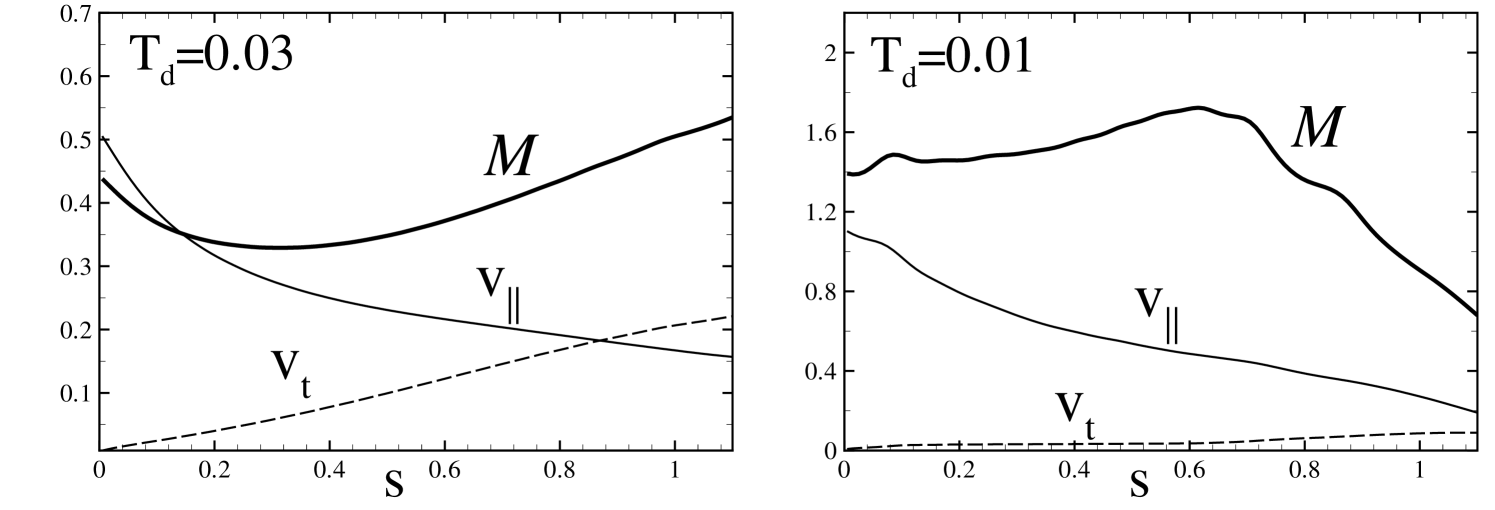
  Fig. 5.—: Distribution of velocities along a magnetic field line going approximately through the middle of the funnel stream obtained at $\Theta=15^{\circ}$. Variable $s$ is the linear distance along this magnetic field line, with $s=0$ at the surface of the star. Here, $v_{||}$ is the velocity along the field line, $v_{t}$ is the velocity in the perpendicular direction, ${\it M}=v/c_{s}$ is the Mach number based on the total velocity of the flow. The left and right panels show the examples of the subsonic and supersonic flows correspondingly.

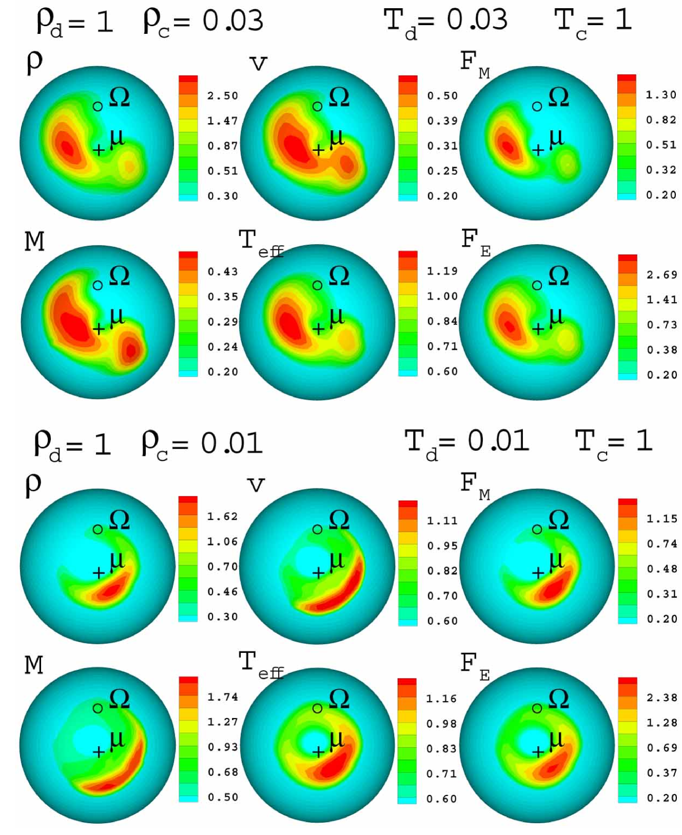
  Fig. 6.—: Distribution of different physical parameters in the hot spots for a misalignment angle $\Theta=30^{\circ}$ and for two types of initial conditions in the disk and corona. $\rho$ is the density, $v$ is the total velocity, $T_{eff}$ is the effective temperature, $\it M$ is the Mach number of the flow, ${\it F}_{M}$ and ${\it F}_{E}$ are the fluxes of mass and energy. The top two rows show the case of higher temperature in the disk and subsonic flow, while the lower two rows show the case of lower temperature in the disk and supersonic flow.

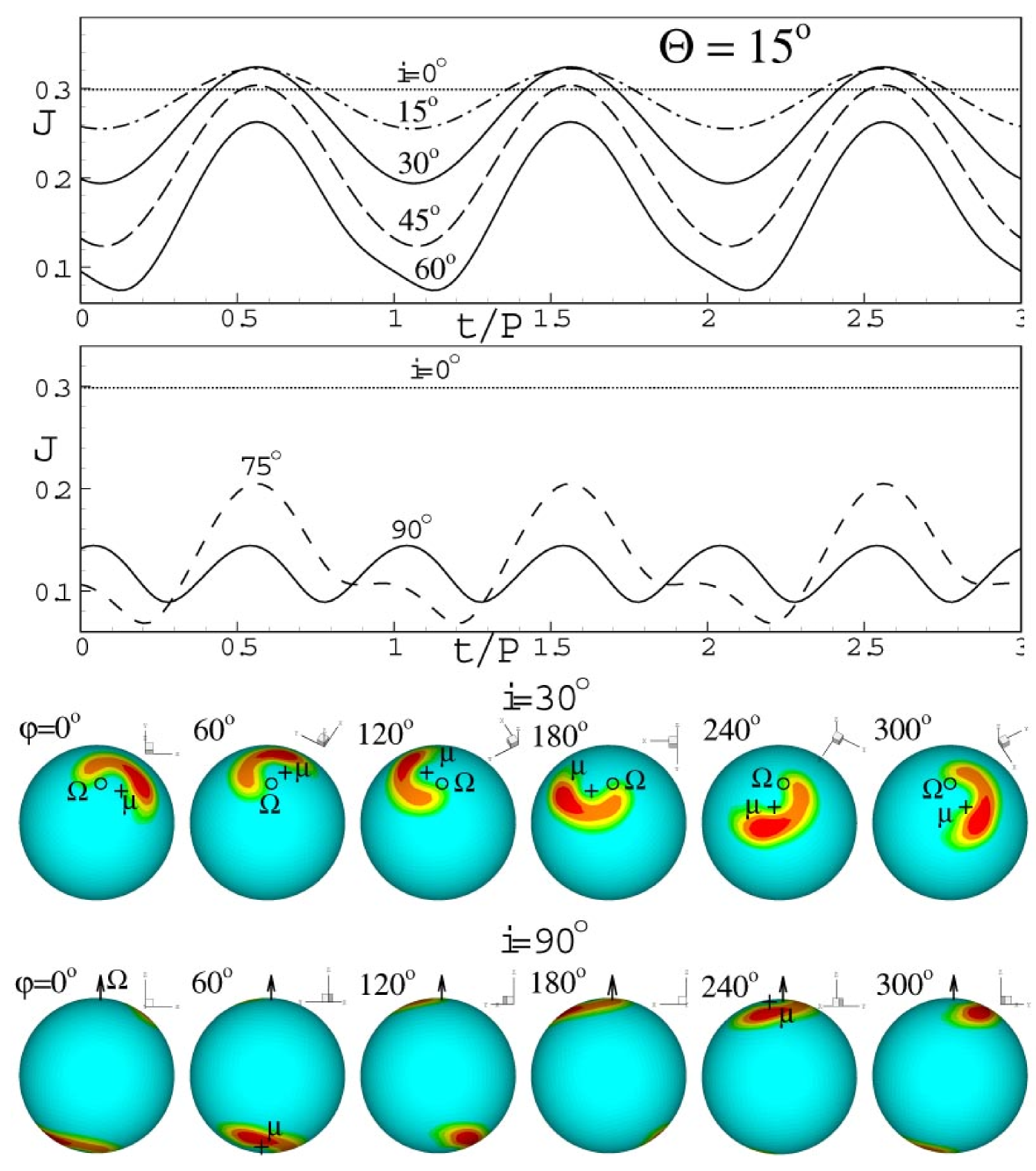
  Fig. 7.—: Light curves calculated for small misalignment angle $\Theta=15^{\circ}$ and for different inclination angles $i$. Time $t$ is measured in periods of rotation of the star $P$. The two bottom pictures show the distribution of energy flux $F(R)$ in the hot spots at different phases $\varphi$ of the star seen by observer at inclination angles $i=30^{\circ}$ and $i=90^{\circ}$. Phases are shown for one period of rotation. The magnetic and rotation axes are marked with a circle and a cross correspondingly.

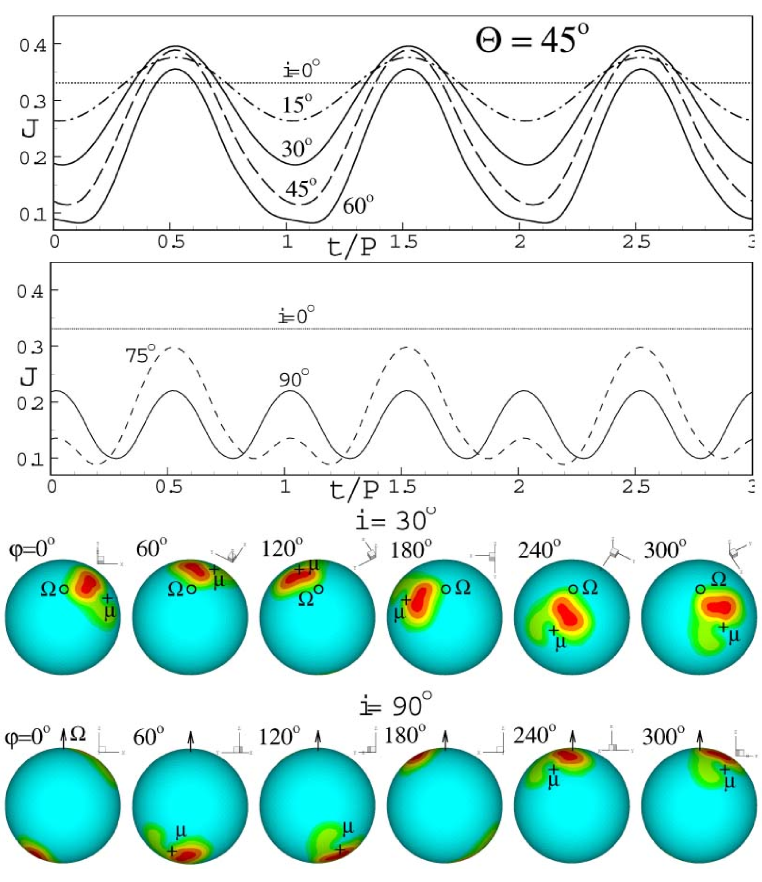
  Fig. 8.—: Light curves calculated for medium misalignment angle $\Theta=45^{\circ}$ and for different inclination angles $i$. All features of the plot are the same as in Figure 7.

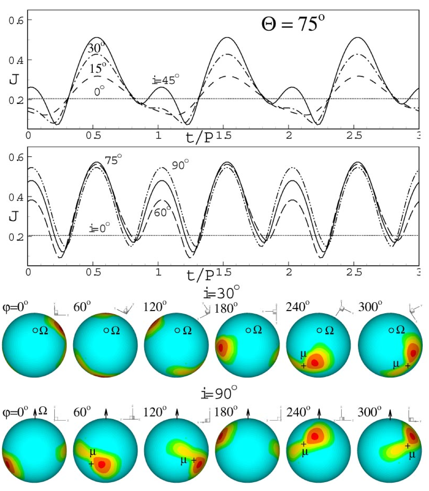
  Fig. 9.—: Light curves calculated for a large misalignment angle $\Theta=75^{\circ}$ and for different inclination angles $i$. All features of the plot are the same as in Figure 7.

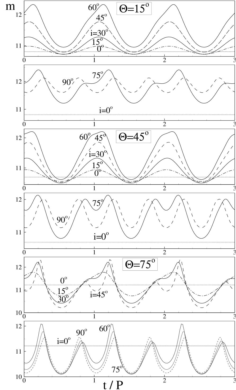
  Fig. 10.—: Light curves similar to those of Figures 7-9, but the intensity is measured in stellar magnitudes $m$. The top two panels correspond to $\Theta=15^{\circ}$, the middle panels correspond to $\Theta=45^{\circ}$ and the bottom two panels correspond to $\Theta=75^{\circ}$.

3.4 Energy Flux and Temperature in the Spots

Matter flowing to the star in an accretion stream carries both kinetic and thermal energies. The associated energy flux through the surface of the star at the point ${\bf R}$ is:

$$F_{E}({\bf R})=\rho~{}\hat{\bf n}\cdot{\bf v}\left({1\over 2}{{\bf v}^{2}+w}\right),$$

where, ${\bf v}$ is the velocity of plasma relative to the surface of the star, $w=\gamma(p/\rho)/(\gamma-1)$ is the specific enthalpy of the plasma, and $\hat{\bf n}=-\hat{\bf r}$ is the inward pointing normal to the surface of the star.

The detailed physics of the hot spots is complicated. To calculate the spectrum of radiation from the hot spots an analysis of the radiation transfer is needed (see, e.g., Lamzin 1998; Muzerolle, Hartmann, & Calvet 1998; Muzerolle, Calvet, & Hartmann 2001). This paper does not include an analysis of the radiation transfer. We obtain approximate temperature distributions in the hot spots based on overall energy conservation. Namely, we assume that energy released in the hot spots is due to the energy flux of equation (2). At the point ${\bf R}$ of the surface of the star, this energy flux is considered to radiate as a black body. Thus, $F_{E}({\bf R})=\sigma T_{\rm eff}^{4}$, where $\sigma=5.67\times 10^{-5}({\rm erg/s})/{\rm cm}^{2}/{\rm K}^{4}$ is a Stephan-Boltzmann constant and $T_{\rm eff}$ is the effective black-body temperature of the radiation. Thus, we get

$$T_{\rm eff}({\bf R})=\left[{\rho~{}\hat{\bf n}\cdot{\bf v}\over\sigma}\left({1\over 2}{{\bf v}^{2}+w}\right)\right]^{1/4}.$$

Figure 6 shows the distribution of $F_{\rm E}$ and $T_{\rm eff}$ in the spots. Their shapes are similar to those of the density. The distribution of $T_{\rm eff}$ is important for understanding the variability in different spectral bands. The spots are expected to be smaller at higher $T_{\rm eff}$ and larger at lower $T_{\rm eff}$. An indication of such distribution was possibly observed in the CTTS object BP Tauri, where the area of the hot spots was estimated to be different when different methods were used. Errico, Lamzin & Vittone (2001) estimated the area to be $20\%$ of the surface of the star. They used the spectral lines which are thought to originate in the external regions of the funnel flow. Ardila & Basri (2000) estimated the area to be much smaller, $0.3\%$. However, they modelled the UV continuum, which originates in the hottest region of the spots. Note that in present analysis, we do not take into account the radiation coming from the interior of the star.

4 The Intensity of Radiation and Light Curves

For calculation of the radiation intensity from the hot spots, we suppose that all of the kinetic energy flux $F_{E}({\bf R}$ goes into radiation. The energy, radiated by a unit area of the spot is

$$F_{E}({\bf R})=\int\limits_{\cos{\theta}>0}d\Omega~{}f({\bf R},{\bf m})~{},$$

where $f({\bf R},{\bf m})$ is the intensity of the radiation from a unit area into the solid angle element $d\Omega$ in the direction ${\bf m}$ with ${\bf m}\cdot\hat{\bf r}=\cos\theta$. The condition $\cos\theta>0$ corresponds to the upper half space above the star’s surface. For specificity we consider $f({\bf R},{\bf m})=A({\bf R})\cos{\theta}.$ Thus we obtain the luminosity of unit area at point ${\bf R}$,

$$F_{E}({\bf R})=2\pi A({\bf R})\int\limits_{0}^{\pi/2}\sin{\theta}\cos{\theta}d{\theta}=\pi A({\bf R})~{},$$

and

$$f({\bf R},{\bf m})={1\over\pi}{F_{E}({\bf R})\cos{\theta}}~{}.$$

Consider now the intensity of radiation seen by a distant observer. The unit vector from the star to the observer is denoted $\hat{\bf k}$. This vector makes an angle $\beta$ with the normal to the star’s surface, that is, $\cos\beta=\hat{\bf k}\cdot\hat{\bf r}$. The intensity of radiation in the direction $\hat{\bf k}$ is obtained by integrating over the stellar surface,

$$J=\int{dS~{}f({\bf R},{\hat{\bf k}})}=\frac{1}{\pi}\int\limits_{\cos{\beta}>0}dS~{}F_{E}({\bf R})\cos{\beta}~{},$$

where $dS$ is an element of the surface area of the star. The condition $\cos{\beta}>0$ or $\beta<\pi/2$ corresponds to only the near side of the star being visible. The rotation of a star with hot spots leads to variations in the observed emission $J$.

4.1 Variability Curves at Fixed position of Spots

Hot spots constantly change their shape and position. However, in many situations the changes are small (e.g., in case of the cooler disk), so that as a first step we suppose that the spots have fixed location at the surface of the star and variability is connected with rotation of the star relative to the fixed observer. This approach helps to understand different features of the light curves, associated with structure and location of the hot spots at different $\Theta$. Examples of actual variability curves are shown in §4.2.

We consider one of the initial conditions (warmer disk, $T_{d}=0.03$), take hot spots at a single moment of time, $t=5P_{0}$ (as in Figure 1), and calculate from equation (6) the observed intensity $J(t)$ as the star rotates. Such light curves were calculated for misalignment angles $\Theta=15^{\circ},~{}45^{\circ}$, and $\Theta=75^{\circ}$, and for different inclination angles of the disk $i$ with respect to the line of sight. The inclination angle of the disk is the angle between the direction of ${\bf\Omega}$ and the direction to the observer $\hat{\bf k}$. That is, $\cos i=\hat{\bf\Omega}\cdot\hat{\bf r}~{}$. The results are shown at Figures 7 - 9.

Figure 7 shows results for a relatively small misalignment angle $\Theta=15^{\circ}$. The top panel shows the light curves for different inclination angles $i$. The bottom panel shows the orientation of the star during one rotation period. The phases are shown for two cases: at $i=30^{\circ}$, which is a probable inclination angle, and at $i=90^{\circ}$ which is edge on.

Of course for $i=0^{\circ}$ there is no variability because the observer sees only one hot spot which rotates around the $\Omega$ axis. For larger inclination angles, $i=15^{\circ}$, $i=30^{\circ}$, $i=45^{\circ}$, dips appear in the light curves which increase with increasing of $i$. These dips are connected with the fact that the hot spots come closer to the edge of the star and are partially obscured. Under these conditions the star will be observed as a variable star with one maximum per period. For $i=60^{\circ}$, the light curve becomes asymmetric and this asymmetry increases for larger inclination angles $i$. This is connected with the fact that the second spot, which was invisible at smaller $i$, appears and starts to contribute to the luminosity. Thus, two intensity maxima per stellar period are observed. The two maxima become of equal amplitude at $i=90^{\circ}$.

Figure 8 shows similar plots, but for the misalignment angle $\Theta=45^{\circ}$. The light curves in this case are similar to those at smaller $\Theta$. However, the shorter time-scale variability appears at large inclination angles at $i\mathrel{\hbox{\hbox to0.0pt{\hbox{\lower 4.0pt\hbox{$\sim$}}\hss}\hbox{$>$}}}75^{\circ}$.

Figure 9 shows the case of a high misalignment angle, $\Theta=75^{\circ}$. For this and larger values of $\Theta$, the double maxima (half-period) variability appears for many inclination angles starting from $i\mathrel{\hbox{\hbox to0.0pt{\hbox{\lower 4.0pt\hbox{$\sim$}}\hss}\hbox{$>$}}}30^{\circ}$.

The figures 7-9 show intensity in dimensionless units. This value in dimensional units will be $J\dot{E}_{0}$, where $\dot{E}_{0}$ is the dimensional energy flux (see §2.3 and §2.4). The value $J\dot{E}_{0}$ gives the energy flux from the spots radiated to the direction of the observer. This value will determine the observed flux, when the distance to the object will be taken into account. Thus, the X-ray flux observed e.g. from millisecond pulsars will be proportional to $J$ and the expected variability curves will be similar to those at the Figures 7-9. However, for CTTS it is common to show the light curves on a logarithmic scale, using the standard stellar magnitude values. As long as this analysis can be applicable to stars at different distances, we accept the random null-point for calculation of $m$ which will be different for different CTTS. We suppose that intensity $J=0.1$ corresponds to $m=12$, and calculate the light curve using the standard formulae: $m=12-2.512(1.+\rm{log}J)$. Figure 10 shows light-curves in stellar magnitudes for different $\Theta$ and $i$. Note that the curves have different shapes which may be used for estimating values of $\Theta$ and $i$.

4.2 Variability Curves for Changing Spots

Here, we present samples of actual variability curves. We take the data for all moments of time from the numerical simulations. The star rotates slowly, with $\Omega_{*}=0.19$, so that one rotation of the star corresponds to $5.26$ rotations of the inner radius of the disk $P_{*}\approx 5.3P_{0}$. Thus, to show the variability pattern during few rotations of the star, we need pretty long runs. Here, we show sample results from several relatively long runs with $t=15-16P_{0}$. Figure 11 shows sample light curves for the case of the cooler disk, and $\Theta=15^{\circ}$ and $\Theta=45^{o}$. One can see that the “real” light curves have similar features to the curves for fixed hot spots. However, the variability pattern departs from the exact variability patterns shown at Figures 7 and 8. This is because the hot spots continue to change their shape and position. Figure 12 shows variability curves for larger misalignment angles, $\Theta=75^{\circ}$ and $\Theta=90^{o}$ (for warmer disk). One can see that at these misalignment angles, the light curves are closer to those of Figure 9, because the spots have almost fixed positions on the stellar surface.

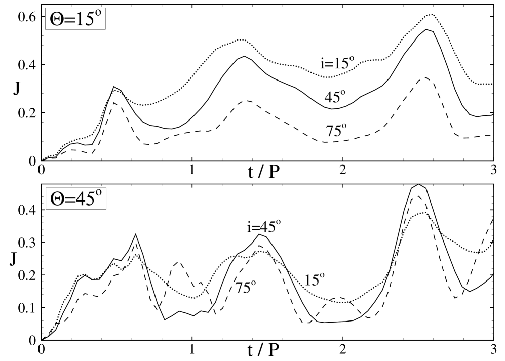
  Fig. 11.—: Light curves calculated for actual time-dependent hot spots for misalignment angles $\Theta=15^{\circ}$ and $\Theta=45^{\circ}$, and for different inclination angles $i$, for the case of the cooler disk, $T_{d}=0.01$.

  Fig. 12.—: Light curves calculated for actual time-dependent hot spots for misalignment angles $\Theta=75^{\circ}$ and $\Theta=90^{\circ}$, and for different inclination angles $i$, for the case of the warmer disk, $T_{d}=0.03$.

5 Discussion

In this paper we fixed parameters of the star and the flow. Below we discuss dependence of the results on $\Omega_{*}$ and on the accretion rate $\dot{M}$. In §5.2 we discuss the limitations of the model and future work.

5.1 Dependence of Results on Parameters of the Star and the Disk

$\Omega$–Dependence: For the results given here we have taken a relatively low angular velocity, $\Omega_{*}=0.19$. This corresponds to CTTS with a period $P=9.4~{}{\rm days}$. We did additional simulations for an intermediate angular velocity, $\Omega_{*}=0.35$ ($P=3.3~{}{\rm days}$), and a rapidly rotating star, $\Omega_{*}=1.0$ ($P=1.8~{}{\rm days}$). We observed that the hot spot shapes are similar for slowly and for rapidly rotating stars. For the intermediate angular velocity, the bow shape is less prominent. The bow shape of the hot spots reflects the typical shape of the funnel streams which have a thickness that is small compared with their width. This is typical for relatively small inclination angles, $\Theta\mathrel{\hbox{\hbox to0.0pt{\hbox{\lower 4.0pt\hbox{$\sim$}}\hss}\hbox{$<$}}}30^{\circ}$, where the stream should “climb” an appreciable distance above the equatorial plane before accreting to the vicinity of the magnetic pole. At small inclination angles, the bow shape is natural, because it may be considered as a part of the narrow cylindrical ring which occurs for $\Theta=0$.

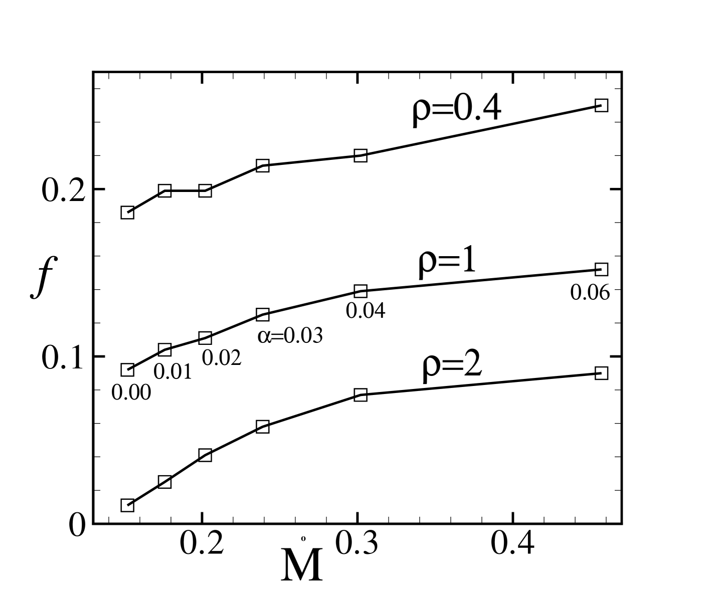
  Fig. 13.—: The fraction of the star covered by the hot spots at the density levels: $\rho=0.4$, $\rho=1$, and $\rho=2$ as a function of the accretion rate $\dot{M}$. Squares show separate runs at different $\alpha$ parameters of the disk viscosity.

$\dot{M}$–Dependence: We studied the dependence of the size of the spots on the accretion rate $\dot{M}$. We introduced an alpha-type viscosity analogous to one used in R02 and performed a set of runs at different values of accretion rate $\dot{M}$ (different $\alpha$). Figure 13 shows that the fraction ${\it f}$ of the star covered by the hot spots increases with the accretion rate for a range of density levels, $\rho=0.4,1,2$. Thus, the size of the spots increases as the accretion rate increases. This is in accord with recent results of Ardila and Basri (2000), who analyzed the UV variability of the CTTS BP Tau and have shown significant correlation between the accretion rate and the filling factor of the shocks. In R03 we noticed that at a larger accretion rate, the streams become wider and cover a larger area of the magnetosphere. This may possibly explain the observed variation of the shapes of magnetospheric lines with the accretion rate (Muzerolle et al. 2001).

5.2 Limitations of the Model and Future Work

Variability in different spectral lines in the accreting magnetized stars may be associated with different regions: inner regions of the disk, magnetospheric streams, hot spots, or outflows. In this paper we analyze only the variability due to the rotation of the hot spots, while the variability associated with other regions will be investigated in the future work. The light from the hot spots may be also obscured by magnetospheric streams or by the warped inner regions of the disk if the star is approximately edge-on (e.g., Bouvier, et al. 1999, 2003). This paper does not include the effect of obscuration. The warping of the inner regions of the disk (Aly 1980, Lipunov & Shakura 1980, Lai 1999) was not observed in the simulations, but a special set of simulations will be done for investigation of this possible phenomenon.

The magnetic field of the CTTS or millisecond pulsars may not be a pure dipole field (Safier 1998; Smirnov et al. 2003). This can lead to more complicated geometry of the hot spots and more complicated variability patterns. However, the detailed analysis of the photometric and spectral variability of a number of CCTS have shown that most of the observed features can be explained by models with a dipole magnetic field (e.g., Muzerolle, Hartmann, & Calvet 1998; Petrov, et al. 2001a,b; Alencar, Johns-Krull, & Basri 2001; Bouvier et al. 2003). This paper considers only the case where the star’s field is a dipole field. Non-dipolar field geometries will be investigated separately.

We observed that the hot spots may rotate more rapidly or more slowly than the star, which will lead to quasi-periodic oscillations in the light curves and may explain QPOs observed in CTTS (see Smith, Bonnell, & Lewis 1995) and millisecond pulsars (see, e.g., Chakrabarty et al. 2003). QPO variability in the disk-magnetized star systems may also be associated with oscillations of the inner radius of the disk (e.g., Goodson, Winglee & Böhm 1997). We plan to further investigate the quasi-variability associated with such phenomena.

6 Summary

Disk accretion to a rotating star with a misaligned dipole magnetic field has been studied further by three-dimensional MHD simulations. This work focuses on the nature of the “hot spots” formed on the stellar surface due to the impact of two or more funnel streams. We investigated the shape and intensity of the hot spots for different misalignment angles $\Theta$ between the star’s rotation axis $\bf\Omega$ and its magnetic moment ¯. Further, we calculated the light curves due to rotation of the hot spots for different angles $i$ between the observer’s line-of-sight and $\bf\Omega$. The main results are the following:

1. For small inclination angles, $\Theta<30^{\circ}$, the hot spots typically have a shape of a bow which is bent around the magnetic pole. At large inclination angles, $\Theta\mathrel{\hbox{\hbox to0.0pt{\hbox{\lower 4.0pt\hbox{$\sim$}}\hss}\hbox{$>$}}}60^{\circ}$, the shape becomes bar-like. Often a spot on a given hemisphere splits to form two spots, which reflects the splitting of the funnel stream into two streams. The secondary stream is typically weaker than the main stream so that one spot is much larger than the other.

2. The density, temperature, matter flux and other parameters increase towards the central regions of the spots, so that the spots are larger at lower temperature/density and smaller at larger temperature/density. They cover about $10-20\%$ of the area of the star at the density level typical for the external regions of the funnel streams (see Figures 1 and 2). The size of the hot spots increases with the accretion rate.

3. The spots have tendency to be located close to the $\mu-\Omega$ plane. They tend to be located downstream of this plane if a star rotates slowly (i.e., the inner region of the disk and the foot-points of the stream rotate somewhat faster than the star), or upstream, if a star rotates relatively fast. The spots wander around their “favorite” position. The amplitude of wandering is smaller in case of the cooler disk.

4. The calculated light curves reveal the following features:

(a). The light curve has one peak per one period of rotation of the star and the shape is approximately sinusoidal. This is typical for small and medium misalignment angles, $\Theta\mathrel{\hbox{\hbox to0.0pt{\hbox{\lower 4.0pt\hbox{$\sim$}}\hss}\hbox{$<$}}}45^{\circ}$, and inclination angles $i\mathrel{\hbox{\hbox to0.0pt{\hbox{\lower 4.0pt\hbox{$\sim$}}\hss}\hbox{$<$}}}60^{\circ}$.  (b). The light curve has two peaks per period of rotation. This is typical for all $\Theta$ if inclination angle is large, $i>75^{\circ}$. At very large misalignment angles, $\Theta\mathrel{\hbox{\hbox to0.0pt{\hbox{\lower 4.0pt\hbox{$\sim$}}\hss}\hbox{$>$}}}60^{\circ}-70^{\circ}$, the double-peak curve is typical for wide range of inclination angles, $i\mathrel{\hbox{\hbox to0.0pt{\hbox{\lower 4.0pt\hbox{$\sim$}}\hss}\hbox{$>$}}}30^{\circ}$.

5. The variation of the shape and location of the spots will lead to departure from the exact variability and to quasi-variability. At small misalignment angles, $\Theta<30^{\circ}$, the streams (and hot spots) may rotate with velocity different from that of the star (R03) thus leading to quasi-periodic oscillations.

This research was conducted using the resources of the Cornell Theory Center, which receives funding from Cornell University, New York State, Federal Agencies, foundations, and corporate partners. This work was supported in part by NASA grants NAG5-13220, NAG5-13060, and by NSF grant AST-0307817. AVK and GVU were partially supported by grants INTAS CALL2000-491, RFBR 03-02-16548, by contract MIST # 40.022.1.1.1106 and by Russian program “Astronomy”. The authors thank Drs. S.A. Lamzin and P.P. Petrov for discussion of CTTS, Drs. D. Chakrabarty and D. Lai for discussion of millisecond pulsars, to Dr. J. Stinchcombe for editing the manuscript and to the referee for valuable suggestions.

REFERENCES

Alencar, S.H.P., Johns-Krull, C.M., & Basri, G. 2001, AJ, 122, 3335

Aly, J.J. 1980, Astron. & Astrophys., 86, 192

Ardila, D.R., Basri, G., 2000, ApJ 539, 834

Bertout, C., Basri, G., & Bouvier, J. 1988, ApJ, 330, 350

Bildsten, L., et al. 1997, ApJS, 113, 367

Bouvier, J., Bertout, C., Bouchet, P., 1986, A&A 158, 149

Bouvier, J. & Bertout, C. 1989, A&A, 211, 299

Bouvier J., Cabrit S., Fernandez M. et al., 1993, A&A 272, 146

Bouvier, J., Chelli, A., Allain, S., et al. 1999, A&A, 349, 619

Bouvier, J., Grankin, K.N., Alencar, S.H.P., et al. 2003, A&A, 409, 169

Calvet, N., Gullbring, E., 1998, ApJ 509, 802

Camenzind, M. 1990 in: Rev. Mod. Astron. 3, ed. G. Klare, Springer-Verlag (Heidelberg), 234

Chakrabarty, D., Morgan, E.H., Muno, M.P., Galloway, D.K., Wijnands, R., Van Der Klis, M., & Markwardt, G.B. 2003, Nature, 424, 42

Deeter, J.E., et al. 1998, ApJ, 502, 802

Errico, L., Lamzin, S.A., & Vittone, A.A. 2001, A&A 377, 557

Ghosh, P., & Lamb, F.K. 1979, ApJ, 234, 296

Gullbring, E., Calvet, N., Muzerolle, J., & Hartmann, L., 2000, ApJ 544, 927

Goodson, A.P., Winglee, R. M., & Böhm, K.-H., 1997, ApJ, 489, 199

Hartmann,L., Hewett, R., & Calvet, N. 1994, ApJ, 426, 669 1994

Hartmann, L., “Accretion Processes in Star Formation”, Cambridge University Press, 1998

Hayashi, M.R., Shibata, K., & Matsumoto, R. 1996, ApJ, 468, L37

Herbst, W. et al. 1986, ApJ, 310, L71

Herbst, W., Koret, D.L. 1988, AJ 96, 1949

Koldoba, A.V., Romanova, M.M. , Ustyugova, G.V., & Lovelace, R.V.E. 2002, ApJ, 576, L53

Königl, A. 1991, ApJ, 370, L39

Lai, D. 1999, ApJ, 524, 1030

Lamzin, S.A. 1995, Ap.Sp.Sci. 224, 211

Lamzin, S.A. 1998, Astron. Reports 42, 322

Lipunov, V. M., & Shakura, N.I. 1980 , Sov. Astron. Lett., 6, 14

Livio, M. & Pringle, J.E. 1992, MNRAS, 259, 23

Miller, K.A. & Stone, J.M. 1997, ApJ, 489, 890

Muzerolle, J, Hartmann, L., & Calvet, N. 1998, ApJ, 116, 455

Muzerolle, J, Calvet, N., & Hartmann, L. 2001, ApJ, 550, 944

Petrov, P.P., Gahm, G.F., & Gameiro, J.F., Duemmler, R., Ilyin, I.V., Laakkonen, T., Lago, M.T.V.T., & Tuominen, I. 2001a, A&A, 369, 993

Petrov, P.P., Pelt, J., & Tuominen, I. 2001b, A&A, 375, 993

Petrov, P.P. 2004, Astrofizika, in press

Romanova, M.M., Ustyugova, G.V., Koldoba, A.V., & Lovelace, R.V.E. 2002, ApJ, 578, 420 (R02)

Romanova, M.M., Ustyugova, G.V., Koldoba, A.V., & Lovelace, R.V.E. 2003, ApJ, 595, 1009 (R03)

Safier, P.N. 1998, ApJ, 494, 336

Shu, F.H., Najita, J., Ostriker, E.C., Wilkin, F., Ruden, S.P., & Lizano, S. 1994, ApJ, 429, 781

Smirnov, D.A., Fabrika, S.N., Lamzin, S.A., & Valyavin, G.G. 2003, A&A, 401, 1057

Smith, K.W., Bonnel, I.A., & Lewis, G.F. 1995, MNRAS, 276, 263

Trümper, J., Kahabka, P., $\ddot{O}$gelman, H., Pietsch, W., & Voges, W. 1986, ApJ, 300, L63

Warner, B. 1995, Cataclysmic Variable Stars (Cambridge: Cambridge Univ. Press)

Warner, B. 2000, The Publications of the Astronomical Society of the Pacific, Volume 112, Issue 778, p. 1523

Wickramasinghe, D. T., Wu, K., & Ferrario, L. 1991, MARAS, 249, 460