Anthropic predictions for vacuum energy and neutrino masses

Abstract

It is argued that the observed vacuum energy density and the small values of the neutrino masses could be due to anthropic selection effects. Until now, these two quantities have been treated separately from each other and, in particular, anthropic predictions for the vacuum energy were made under the assumption of zero neutrino masses. Here we consider two cases. In the first, we calculate predictions for the vacuum energy for a fixed (generally non-zero) value of the neutrino mass. In the second we allow both quantities to vary from one part of the universe to another. We find that the anthropic predictions for the vacuum energy density are in a better agreement with observations when one allows for non-zero neutrino masses. We also find that the individual distributions for the vacuum energy and the neutrino masses are reasonably robust and do not change drastically when one adds the other variable.

I Introduction

The smallness of the vacuum energy density $\rho_{\Lambda}$ (the cosmological constant) is one of the most perplexing mysteries that we now face in theoretical physics. The values of $\rho_{\Lambda}$ indicated by particle physics models are far too large, at least by 60 orders of magnitude. The only plausible explanation that has so far been suggested is that $\rho_{\Lambda}$ is a stochastic variable, taking different values in different parts of the Universe, and that the smallness of the observed value is due to anthropic selection effects. The proposed selection mechanism is very simple [1, 2, 3, 4, 5, 6, 7, 8]. The growth of density fluctuations leading to galaxy formation effectively stops when the vacuum energy dominates the Universe. In regions where $\rho_{\Lambda}$ is greater, it will dominate earlier, and thus there will be fewer galaxies (and therefore fewer observers). Suppose ${\tilde{\rho}_{\Lambda}}$ is the value for which the vacuum energy dominates at about the epoch of galaxy formation, $z_{\Lambda}\sim z_{G}$. Then, values $\rho_{\Lambda}\gg{\tilde{\rho}_{\Lambda}}$ will be rarely observed, because the density of galaxies in the corresponding regions is very low. On the other hand, values $\rho_{\Lambda}\ll{\tilde{\rho}_{\Lambda}}$ are also rather unlikely, simply because this range of values is very small. (This argument assumes that the prior distribution for $\rho_{\Lambda}$ is not sharply peaked at $\rho_{\Lambda}=0$; see below.) Thus, a typical observer should expect to measure $\rho_{\Lambda}\sim{\tilde{\rho}_{\Lambda}}$: the vacuum energy should dominate roughly at the epoch of galaxy formation.

This anthropic prediction was subsequently confirmed by supernovae and CMB observations. The observed value [12, 13] for the vacuum energy density, in units of the critical density, $\Omega_{\Lambda}^{obs}\approx 0.7$, is in a qualitative agreement with the anthropic probability distribution, which is peaked at [2, 3, 6, 7] $\Omega_{\Lambda}\sim 0.9$. The most recent analysis [8] finds that anthropic predictions are in agreement with observations at a $2\sigma$ level.

Here we show that the agreement can be further improved by allowing for a nonzero neutrino mass. The value $\tilde{\rho}_{\Lambda}$ at the peak of the probability distribution for $\rho_{\Lambda}$ depends on the magnitude of density fluctuations on the galactic scale, $\sigma_{G}$. The calculation in [8] was performed assuming massless neutrinos and a scale-invariant spectrum of fluctuations, normalized using the large-scale CMB measurements. If $\sigma_{G}$ is decreased, galaxies form later, and $\tilde{\rho}_{\Lambda}$ becomes smaller, thus improving the agreement with $\rho_{\Lambda}^{obs}$. This is precisely the effect of massive neutrinos, since they slow down the growth of density fluctuations. If the sum of the three neutrino masses is $m_{\nu}\sim 1-2$ eV, this suppression is sufficiently large to bring the anthropic prediction for $\rho_{\Lambda}$ into agreement with observations at the $1\sigma$ level.

It is very intriguing that the value $m_{\nu}\sim 1$ eV for the sum of the neutrino masses was itself recently predicted from anthropic considerations. It was suggested in [14] that the neutrino masses might also be stochastic variables, changing from one part of the Universe to another, and that their small values might be due to anthropic selection. In regions with a larger value of $m_{\nu}$, the suppression of density fluctuations is stronger. As a result, there are fewer galaxies in such regions, and the corresponding values of $m_{\nu}$ are less likely to be observed. The probability distribution for $m_{\nu}$ calculated in [14] is peaked at $m_{\nu}\approx 2$ eV, with a $1\sigma$ range between 0.5 eV and 3 eV. This corresponds to a mild but non-negligible suppression of galaxy formation. Indeed, recent analysis of X-ray cluster data combined with CMB and 2dF has suggested that $m_{\nu}=0.64^{+0.40}_{-0.28}$ eV [16], although this remains controversial given cluster-related systematic uncertainties [31]. In this paper, we shall also consider models where both $m_{\nu}$ and $\rho_{\Lambda}$ are assumed to be stochastic variables.

The paper is organized as follows. In Section II we describe our general approach and justify our choice of the theoretical prior distributions for $m_{\nu}$ and $\rho_{\Lambda}$. In Section III we calculate the probability distribution for $\rho_{\Lambda}$ at nonzero values of $m_{\nu}$, as well as the joint probability distribution for $m_{\nu}$ and $\rho_{\Lambda}$ in models where both are variable. We conclude with a discussion of our results in Section IV. Some technical details are given in the Appendix.

II The method and the priors

The method used in this paper follows closely that in [7, 14]. Consider a model in which $m_{\nu}$ and $\rho_{\Lambda}$ are allowed to vary from one part of the Universe to another. We define the probability distribution ${\cal P}(m_{\nu},\rho_{\Lambda})dm_{\nu}d\rho_{\Lambda}$ as being proportional to the number of observers in the Universe who will measure $m_{\nu}$ in the interval $dm_{\nu}$ and $\rho_{\Lambda}$ in the interval $d\rho_{\Lambda}$. This distribution can be represented as [2, 7, 14]

$${\cal P}(m_{\nu},\rho_{\Lambda}) \propto {\cal P}_{prior}(m_{\nu},\rho_{\Lambda})$$ (1)

$$\times \int dM\ n_{G}(m_{\nu},\rho_{\Lambda},M)\ N_{obs}(m_{\nu},\rho_{\Lambda},M).$$ (2)

Here, ${\cal P}_{prior}(m_{\nu},\rho_{\Lambda})dm_{\nu}d\rho_{\Lambda}$ is the prior distribution, which is proportional to the comoving volume of those parts of the Universe where $m_{\nu}$ and $\rho_{\Lambda}$ take values in intervals $dm_{\nu}$ and $d\rho_{\Lambda}$, $n_{G}(m_{\nu},\rho_{\Lambda},M)dM$ is the comoving number density of galaxies of mass in the interval $dM$ that will ever form in regions with given values of $m_{\nu}$ and $\rho_{\Lambda}$, and $N_{obs}(m_{\nu},\rho_{\Lambda},M)$ is the average number of observers per galaxy. The distribution (2) gives the probability that a randomly selected observer is located in a region where the sum of the three neutrino masses is in the interval $dm_{\nu}$ and the vacuum energy density is in the interval $d\rho_{\Lambda}$.

We shall assume, as it was done in [6, 7, 14], that the integral in (2) is dominated by large galaxies like the Milky Way, with mass $M\gtrsim M_{G}\sim 10^{12}M_{\odot}$. We shall also assume, as a rough approximation, that for galaxies in this mass range $N_{obs}$ does not depend significantly on $m_{\nu}$ or $\rho_{L}$ and is simply proportional to the number of stars, or to the mass of the galaxy,

$$N_{obs}(m_{\nu},\rho_{\Lambda},M)\propto M\ .$$ (3)

(We shall comment on the validity of this assumption in Section IV.) Then it follows from Eq. (2) that

$${\cal P}(m_{\nu},\rho_{\Lambda})\propto{\cal P}_{prior}(m_{\nu},\rho_{\Lambda})F(M>M_{G},m_{\nu},\rho_{\Lambda}),$$ (4)

where $F(M>M_{G},m_{\nu},\rho_{\Lambda})$ is the fraction of matter that clusters into objects of mass larger than $M_{G}$ in regions with these values of $m_{\nu}$ and $\rho_{\Lambda}$.

The fraction of collapsed matter $F(M>M_{G},m_{\nu},\rho_{\Lambda})$ can be approximated using the standard Press-Schechter formalism [17]. We assume a Gaussian density fluctuation field $\delta({\bf x},t,m_{\nu},\rho_{\Lambda})$ with a variance $\sigma(t,m_{\nu},\rho_{\Lambda})$ on the galactic scale $(M_{G}=10^{12}M_{\odot})$,

$$P(\delta,t,m_{\nu},\rho_{\Lambda})\propto\exp\left[-{\delta^{2}\over{2\sigma^{2}(t,m_{\nu},\rho_{\Lambda})}}\right].$$ (5)

At early times, when neutrinos are still relativistic, the variance $\sigma$ is assumed to be independent of $m_{\nu}$ and $\rho_{\Lambda}$. An overdense region collapses when the linearized density contrast $\delta$ exceeds a critical value $\delta_{c}$, which in the spherical collapse model with massless neutrinos is estimated to be [1] $\delta_{c}\approx 1.63$. We shall assume that the same value applies when neutrinos have a small mass.

In the Press-Schechter approximation, the asymptotic mass fraction in galaxies of mass $M>M_{G}$ is

$$F(M>M_{G},m_{\nu},\rho_{\Lambda}) \propto {\rm erfc}\,\left[{X\over\sqrt{2}}\right],$$ (6)

where

$$X=\delta_{c}/{\sigma_{\infty}(m_{\nu},\rho_{\Lambda})}$$ (7)

and $\sigma_{\infty}(m_{\nu},\rho_{\Lambda})\equiv\sigma(t\to\infty,m_{\nu},\rho_{\Lambda})$.

A Prior distributions

The calculation of the prior distribution ${\cal P}_{prior}(m_{\nu},\rho_{L})$ requires a particle physics model which allows the neutrino masses and the dark energy density to vary and a cosmological “multiverse” model that would generate an ensemble of sub-universes with different values of $m_{\nu}$ and $\rho_{\Lambda}$. Let us first focus on the neutrino masses. (The discussion in this subsection follows [18, 14].)

Dirac-type neutrino masses can be generated if the Standard Model neutrinos $\nu^{\alpha}$ mix through the Higgs doublet VEV $\Phi$ to some gauge-singlet fermions $\nu_{c}^{\beta}$,

$$g_{\alpha\beta}\Phi{\bar{\nu}}^{\alpha}\nu_{c}^{\beta}.$$ (8)

The couplings $g_{\alpha\beta}$ will generally be variable in string theory inspired models involving antisymmetric form fields $F_{a}$ interacting with branes. (Here, the index $a$ labels different form fields.) $F_{a}$ changes its value by $\Delta F_{a}=q_{a}$ across a brane, where $q_{a}$ is the brane charge. In the low-energy effective theory, the Yukawa couplings $g_{\alpha\beta}$ become functions of the form fields,

$$g_{\alpha\beta}=\sum g_{\alpha\beta}^{a}{{(F_{a}-F_{a}^{(0)})}\over{M_{p}^{2}}}+...$$ (9)

Here, the summation is over all form fields, the coefficients $g_{\alpha\beta}^{a}$ are assumed to be numbers $\sim 1$, and $M_{p}$ is the effective cutoff scale, which we assume to be the Planck mass. We have assumed that $g_{\alpha\beta}$ vanish at some point $F_{a}=F_{a}^{(0)}$ in the $F$-space; then Eq. (9) is an expansion about that point.

In such models, closed brane bubbles nucleate and expand during inflation [19], creating exponentially large regions with different values of the neutrino masses. When $F_{a}$ changes in increments of $q_{a}$, $m_{\nu}$ changes in increments of $\Delta m_{\nu}\sim\Phi q_{a}/M_{p}^{2}$. To be able to account for neutrino masses $\lesssim 1$ eV, we have to require that $\Delta m_{\nu}\lesssim 1$ eV, that is,

$$q_{a}\lesssim 10^{-11}M_{p}^{2},$$ (10)

for at least some of the brane charges. Such small values of the charges can be achieved using the mechanisms discussed in [20, 21, 22].

The natural range of variation of $F_{a}$ in Eq. (9) is the Planck scale, and the corresponding range of the neutrino masses is $0\leq m_{\nu}^{(i)}\lesssim\Phi$. (Here, the index $i$ labels the three neutrino mass matrix eigenvalues.) Only a small fraction of this range corresponds to values of anthropic interest, $m_{\nu}\lesssim 10$ eV. In this narrow anthropic range, we expect that the probability distribution for $F_{a}$ after inflation is nearly flat [23],

$$d{\cal P}_{prior}\propto dF_{1}dF_{2}...,$$ (11)

and that the functions $g_{\alpha\beta}(F_{a})$ are well approximated by linear functions (9). If all three neutrino masses vary independently, this implies that

$$d{\cal P}_{prior}\propto dm_{\nu}^{(e)}dm_{\nu}^{(\mu)}dm_{\nu}^{(\tau)}.$$ (12)

The probability for the combined mass $m_{\nu}=\sum m_{\nu}^{(i)}$ to be between $m_{\nu}$ and $m_{\nu}+dm_{\nu}$ is then proportional to the volume of the triangular slab of thickness $\sim dm_{\nu}$ in the 3-dimensional mass space,

$$d{\cal P}_{prior}\propto m_{\nu}^{2}dm_{\nu}.$$ (13)

Alternatively, the neutrino masses can be related to one another, for example, by a spontaneously broken family symmetry. If all three masses are proportional to a single variable mass parameter, then we expect

$$d{\cal P}_{prior}\propto dm_{\nu}.$$ (14)

To reiterate, the prior distributions (13),(14) are generic if the following two conditions are satisfied: (i) the full range of variation of $m_{\nu}$ is much greater than the anthropic range of interest and (ii) the point $m_{\nu}=0$ is not a singular point of the distribution. The values of $F_{a}$ which make the Yukawa couplings (9) vanish are not in any way special from the point of view of the distribution for $F_{a}$, so there is no reason to expect a singularity at that point, and thus the condition (ii) is likely to be satisfied.

As was shown in [14], the anthropic prediction for the neutrino masses with the prior given by Eq. (13) is in a strong disagreement with current observational bounds. Allowing for a varying $\rho_{\Lambda}$ is unlikely to change this result.

There is also a possibility that the right-handed neutrinos $\nu_{c}^{\beta}$ in (8) have a large Majorana mass $M_{R}\gg\Phi$. In this case, small neutrino masses can be generated through the see-saw mechanism,

$$m_{\nu}\sim g^{2}\Phi^{2}/M_{R}.$$ (15)

If $M_{R}$ is variable, say, within a range $M_{R}\lesssim M_{p}$, then its most probable values are likely to be $\sim M_{p}$, and the prior distribution will favor $m_{\nu}\sim 10^{-6}$ eV. Such extremely small values of $m_{\nu}$ are in conflict with the neutrino oscillation data. In this paper we shall assume Dirac masses with the prior (14).

It should be noted that the Higgs potential and the Higgs expectation value $\Phi$ in (8) will generally be functions of $F_{a}$. Moreover, each field $F_{a}$ contributes a term $F_{a}^{2}/2$ to the vacuum energy density $\rho_{\Lambda}$, and regions with different values of $F_{a}$ will generally have different values of $\rho_{\Lambda}$. However, in the presence of several form fields with sufficiently small charges, variations of all these parameters are not necessarily correlated, and here we shall assume that there is enough form fields to allow independent variation of the relevant parameters. We can then consider sub-ensembles of regions where some of the parameters are variable, while the other are fixed.

In this paper we will be concerned with two models: (i) variable $\rho_{\Lambda}$ at a fixed value of $m_{\nu}$ and (ii) variable $m_{\nu}$ and $\rho_{\Lambda}$, all other parameters being fixed. A line of reasoning similar to that above suggests that, in the anthropically interesting range, the prior distribution for $\rho_{\Lambda}$ should also be flat [4, 5]

$$d{\cal P}_{prior}\propto d\rho_{\Lambda}.$$ (16)

Assuming independent variation of $m_{\nu}$ and $\rho_{\Lambda}$, we then have

$${\cal P}_{prior}(m_{\nu},\rho_{\Lambda})={\rm const}.$$ (17)

We finally comment on the recent work [24, 25, 26] suggesting that string theory involves a large number of form fields $F_{a}$ ($\sim 10^{3}$) and therefore admits an incredibly large number of vacua ($\sim 10^{1000}$) characterized by different particle physics parameters. The spectrum of $\rho_{\Lambda}$ and $m_{\nu}$ could then be very dense even if the brane charges are not small, $q_{a}\sim M_{p}^{2}$. However, in this “discretuum” of vacua, nearby values of $m_{\nu}$ or $\rho_{\Lambda}$ correspond to very different values of the form fields, and we can no longer argue that the prior distribution should be flat in the anthropic range. Calculation of the prior in such a discretuum remains an important problem for future research. In this paper we shall use the distribution (17).

B The full distribution

The full probability distribution can now be obtained from Eqs. (4), (6), and (17),

$${\cal P}(m_{\nu},\rho_{\Lambda})\propto{\rm erfc}\,\left[{X\over\sqrt{2}}\right]\ ,$$ (18)

where $X$ is given by Eq. (7),

$$X=\delta_{c}/{\sigma_{\infty}}.$$ (19)

Depending on the model, the asymptotic density contrast $\sigma_{\infty}$ is a function of $m_{\nu}$ and $\rho_{\Lambda}$ or of $m_{\nu}$ only.

III The probability distribution

Let us consider models where both $\rho_{\Lambda}$ and $m_{\nu}$ are allowed to vary from one part of the Universe to another. We shall calculate the probability distribution expressed in terms of $\rho_{\Lambda}$. We will also state some of our results in terms of

$$\Omega_{\Lambda}=(8\pi G/3)\rho_{\Lambda}h^{-2}\equiv\omega_{\Lambda}h^{-2}\ .$$ (20)

To describe the growth of density fluctuations, it will be convenient to use the ratio

$$x\equiv{\rho_{\Lambda}\over\rho_{M}(t)}={\Omega_{\Lambda}\over\Omega_{M}}(1+z)^{-3}\$$ (21)

as our time variable. The variance $\sigma_{\infty}(m_{\nu},\rho_{\Lambda})$ in Eq. (19) is proportional to the total linear growth factor of the density perturbations,

$$D^{\infty}(f_{\nu},\rho_{\Lambda})\equiv D(f_{\nu},\rho_{\Lambda},x\rightarrow\infty)\ ,$$ (22)

where

$$f_{\nu}\equiv{\Omega_{\nu}\over\Omega_{B}+\Omega_{cdm}+\Omega_{\nu}}$$ (23)

is the neutrino fraction of the total matter density. Hence, the effect of neutrino masses on the fraction $F(M>M_{G},m_{\nu},\rho_{\Lambda})$ in (18) can be taken into account by writing

$$\sigma_{\infty}(m_{\nu},\rho_{\Lambda})=\sigma_{\infty}(0,\rho_{\Lambda}){D^{\infty}(f_{\nu},\rho_{\Lambda})\over D^{\infty}(0,\rho_{\Lambda})}\ ,$$ (24)

where $D^{\infty}(0,\rho_{\Lambda})$ is the total growth factor in regions with $f_{\nu}=0$.

The linear growth factor as a function of redshift can be found numerically, using standard codes such as CMBFAST [27], or analytically, using, e. g. fitting formulae from [28]. We have tested that the two methods give results that agree within a margin of error of a few percent. Technical details related to their evaluation can be found in the Appendix. Throughout this paper we choose to work with the semi-analytical fitting formulae given in Sec. A 2.

We need to relate the asymptotic density contrast $\sigma_{\infty}^{(0)}$ in Eq. (24) to the locally observable quantities. Current CMB measurements do not extend down to the galactic scale, and to sidestep issues related to light-to-mass bias, the galactic density fluctuations are usually inferred by extrapolating from larger scales (on which the effect of neutrino free streaming is unimportant) using a nearly scale-invariant fluctuation spectrum and assuming that the neutrino masses are negligible. The growth factor evaluated in this way overlooks the non-zero massive neutrino fraction $f_{\nu}^{*}$ in our part of the Universe, which is currently unknown but potentially significant. This growth factor, ${\hat{D}}(f_{\nu}^{*},\rho^{*}_{\Lambda},x)$, is evaluated under the assumption that neutrinos are massless, but with $\Omega_{\nu}^{*}$ added to $\Omega_{cdm}$. Here and below, hats indicate the quantities evaluated for our local region assuming massless neutrinos, and superscript “*” indicates the actual local values of these quantities. For example, $x^{*}\approx 2.3$ is the present local value of $x$ and ${\hat{\sigma}}$ is the asymptotic density contrast in our region calculated assuming massless neutrinos. Hence, we can write

$$\sigma_{\infty}(0)=\hat{\sigma}_{\infty}{D^{\infty}(0,\rho_{\Lambda})\over{\hat{D}}^{\infty}(f_{\nu}^{*},\rho_{\Lambda}^{*})}\ ,$$ (25)

where ${\hat{D}}^{\infty}(f_{\nu}^{*},\rho^{*}_{\Lambda})\equiv{\hat{D}}(f_{\nu}^{*},\rho_{\Lambda}^{*},x\rightarrow\infty)$.

To evaluate ${\hat{\sigma}}_{\infty}$, we again note that in the absence of massive neutrinos, the growing mode of density fluctuations is proportional to $D(0,\rho_{\Lambda},x)$. Therefore, the asymptotic density contrast $\hat{\sigma}_{\infty}$ is related to the present value ${\hat{\sigma}}(M)$ via

$$\hat{\sigma}_{\infty} = \hat{\sigma}(M){{\hat{D}}^{\infty}(f_{\nu}^{*},\rho^{*}_{\Lambda})\over{\hat{D}}(f^{*}_{\nu},\rho^{*}_{\Lambda},x^{*})}\ .$$ (26)

Finally, using Eqs. (24), (25) and (26), we can rewrite Eq. (19) as

$$X={\delta_{c}\over\hat{\sigma}(M)}{{\hat{D}}(f_{\nu}^{*},\rho^{*}_{\Lambda},x^{*})\over D^{\infty}(f_{\nu},\rho_{\Lambda})}\ .$$ (27)

Here, ${\hat{\sigma}}(M)$ is the density contrast on the galactic scale $M=10^{12}M_{\odot}$ inferred from the large-scale CMB data assuming massless neutrinos. We emphasize that the actual density contrast should be smaller if indeed the suppression of the galactic density fluctuations due to neutrinos is non-negligible.. To estimate ${\hat{\sigma}}(M)$ we can use the linear power spectrum inferred from measurements of CMB anisotropies. First we need to find the length scale $R_{G}$ corresponding to the mass scale $M=10^{12}M_{\odot}$. It can be found from

$$R(M) = \left({3M\over 4\pi\rho_{0}}\right)^{1/3}$$ (28)

$$\approx 0.951\ \Omega_{M}^{-1.3}h^{-2/3}\left({M\over 10^{12}M_{\odot}}\right)^{1/3}{\rm Mpc}\ ,$$ (29)

where $\rho_{0}\approx 1.88\cdot 10^{-26}\ {\Omega_{M}h^{2}}\ {\rm kg/m}^{3}$ is the mean cosmic density. For $h=0.72$ and $\Omega_{M}=0.27$ this gives

$$R_{G}\approx 1.32\ {\rm h^{-1}Mpc}\ .$$ (30)

The corresponding linearized density contrast ${\hat{\sigma}}_{R_{G}}$ found using WMAP’s best fit power law model [13] is

$${\hat{\sigma}}_{R_{G}}\approx{\hat{\sigma}}(10^{12}M_{\odot})\approx 2.41\pm 0.26\ .$$ (31)

Substituting analytical expressions for ${\hat{D}}(f_{\nu}^{*},\rho_{\Lambda}^{*},x^{*})$ and $D^{\infty}(f_{\nu},\rho_{\Lambda})$, derived in the Appendix (Sec. A 2), into Eq. (27) and using the fact that $x^{*}\gg x_{eq}$ gives

$$X = {\delta_{c}\over\hat{\sigma}(M)}\left({3\over 2}(x_{eq}^{*})^{-1/3}\right)^{1-p}$$ (32)

$$\times \left({1-f_{\nu}\over 1-f_{\nu}^{*}}\right)^{4p/3}\left({\omega_{\Lambda}\over\omega_{\Lambda}^{*}}\right)^{p/3}{G(x^{*})\over[G(\infty)]^{p}}\ ,$$ (33)

where

$$p={1\over{4}}\left(\sqrt{25-24f_{\nu}}-1\right)$$ (34)

and $G(x)$ is the growth factor in a flat universe filled with pressureless matter and vacuum energy, given by [29, 6]:

$$G(x)={5\over 6}\left[{1+x\over x}\right]^{1/2}\int_{0}^{x}{dw\over w^{1/6}(1+w)^{3/2}}\ ,$$ (35)

with the asymptotic value $G(\infty)\approx 1.44$.

The probability distribution ${\cal P}(m_{\nu},\rho_{\Lambda})$ is obtained from Eqs. (18) and (27) and depends on parameters $\rho^{*}$, ${\hat{\sigma}}_{R_{G}}$ and $f_{\nu}^{*}$. The last parameter, the value of $f_{\nu}$ in our part of the Universe, is one of the quantities we are trying to predict. On the other hand, we found that the distribution is not very sensitive to the assumed value $m_{\nu}^{*}$: varying $m_{\nu}^{*}$ between 0.1 and 3 eV changes the location of the peak of distribution functions by no more than $10\%$ percent. This uncertainty can be accounted for by multiplying ${\cal P}(m_{\nu},\rho_{\Lambda})$ by an appropriately chosen prior probability ${\tilde{p}}(m^{*}_{\nu})$, reflecting the current state of our knowledge of the value of $m_{\nu}^{*}$, and integrating over $m^{*}_{\nu}$. Current $95$% upper bound on the sum of neutrino masses, obtained using the WMAP and SDSS data [31], is $m^{*}_{\nu}\lesssim 1.7$ eV. Hence, we choose ${\tilde{p}}(m^{*}_{\nu})$ to be a Gaussian centered at $m^{*}_{\nu}=0$ with a standard deviation of $\sigma_{m^{*}_{\nu}}=0.85eV$. A similar procedure is also needed to account for the uncertainty in our knowledge of $\rho_{\Lambda}^{*}$ and ${\hat{\sigma}}_{R_{G}}$. We compute $\omega_{\Lambda}^{*}=\Omega_{\Lambda}^{*}{h^{*}}^{2}$ using $h^{*}=\bar{h}\pm\sigma_{h}=0.72\pm 0.08$ measured by the HST project [30] and $\Omega_{\Lambda}^{*}=\bar{\Omega}_{\Lambda}\pm\sigma_{\Omega_{\Lambda}}=0.7\pm 0.08$, a conservative estimate from CMB and large-scale structure observations [13, 31]. We take ${\tilde{p}}(\omega_{\Lambda}^{*})$ to be a Gaussian centered at $\bar{\omega}_{\Lambda}^{*}={\bar{\Omega}_{\Lambda}}{\bar{h}}^{2}$, with a standard deviation $\sigma_{\omega_{\Lambda}}=\bar{\Omega}_{\Lambda}2\bar{h}\sigma_{h}+\bar{h}\sigma_{\Omega_{\Lambda}}$. We account for the uncertainty in ${\hat{\sigma}}_{R_{G}}$ taking ${\tilde{p}}({\hat{\sigma}}_{R_{G}})$ to be a Gaussian with the mean and the standard deviation given by Eq. (31). Hence, we have

$${\cal P}(m_{\nu},\rho_{\Lambda}) \rightarrow \int dm_{\nu}^{*}{\tilde{p}}(m_{\nu}^{*})\int d\omega_{\Lambda}^{*}{\tilde{p}}(\omega_{\Lambda}^{*})$$ (36)

$$\times \int d{\hat{\sigma}}_{R_{G}}{\tilde{p}}({\hat{\sigma}}_{R_{G}})\ {\cal P}(m_{\nu},\rho_{\Lambda})\ .$$ (37)

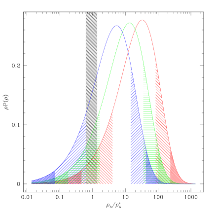
FIG. 1.: The logarithmic probability distributions $\rho_{\Lambda}{\cal P}(m_{\nu},\rho_{\Lambda})$ vs $\rho_{\Lambda}/\rho_{\Lambda}^{*}$ for three fixed values of $m_{\nu}$: $0$, $1$ and $2$ eV, peaked from right to left. In each of the three cases, the lightly and densely shaded areas are the regions excluded at $68$% and $95$% level respectively. Also shown (the dark vertical strip), is the $1\sigma$ uncertainty in $\rho_{\Lambda}^{*}$ derived from observations.

In the following two subsections we consider two cases. In the first, we calculate the probability density for $\rho_{\Lambda}$, while using several fixed values of $m_{\nu}$. In the second, we let both $\rho_{\Lambda}$ and $m_{\nu}$ vary and calculate their joint probability as well as the effective probability for each of the two parameters.

A $P(\rho_{\Lambda})$ for fixed values of $m_{\nu}$

In this subsection we consider a few fixed values of $m_{\nu}$ and evaluate corresponding probabilities for $\rho_{\Lambda}$.

The probability ${\cal P}(\rho_{\Lambda})$ per log $\rho_{\Lambda}$ for $m_{\nu}=0$, $1$ and $2$ eV is shown in Fig. 1 along with the $1$ and $2\sigma$ bounds in the three cases. These bounds are found by cutting off equal measures of probability on both ends ($16$% and $2.5$% for $1$ and $2\sigma$, respectively). Also shown in the figure is the observationally favored range of $\rho_{\Lambda}$. As one can see from the figure, the observed value is within the $2\sigma$ range of the anthropic prediction in all three cases and within the $1\sigma$ bound in the $m_{\nu}=2$eV case.

B Joint probability $P(m_{\nu},\rho_{\Lambda})$

Let us now calculate the probability distribution ${\cal P}(m_{\nu},\rho_{\Lambda})$ with both $m_{\nu}$ and $\rho_{\Lambda}$ variable.

FIG. 2.: The $68\%$ and $95\%$ probability contours in the $m_{\nu}$-$\rho_{\Lambda}$ parameter plane for flat priors. The shaded vertical strip shows the $1\sigma$ uncertainty in the observed value of $\rho_{\Lambda}$.

We are interested in finding the $68\%$ and $95\%$ probability contours in the $m_{\nu}$-$\rho_{\Lambda}$ parameter plane. The simple procedure of cutting off equal measures of probability on both ends used in the previous subsection does not readily generalize to the case of more than one variable. Instead, we find contours of constant logarithmic probability density $m_{\nu}\rho_{\Lambda}{\cal P}(m_{\nu},\rho_{\Lambda})$ that bound $68\%$ and $95\%$ of the volume under the surface defined by the probability distribution ${\cal P}(m_{\nu},\rho_{\Lambda})$. These contours are shown in Fig. 2.

FIG. 3.: Effective logarithmic probability distribution for $m_{\nu}$ and the boundaries of the $68\%$ and $95\%$ probability regions.

The ensemble averaged values of the dark energy density and the neutrino masses found using the joint probability distribution ${\cal P}(m_{\nu},\rho_{\Lambda})$ are

$$\langle\Omega_{\Lambda}\rangle=0.85\ ,\ \langle\rho_{\Lambda}/\rho_{\Lambda}^{*}\rangle=21\ ,\ \langle m_{\nu}\rangle=1.5{\rm eV}\ .$$ (38)

FIG. 4.: The effective probability from Eq. (40) plotted per log $\rho_{\Lambda}/\rho_{\Lambda}^{*}$. The lightly and densly shaded regions are excluded at $1$ and $2\sigma$ level, respectively. Expressed in terms of $\Omega_{\Lambda}$, the $1\sigma$ region is given by $0.695<\Omega_{\Lambda}<0.988$.

Next we find the effective one dimensional probability distributions for $m_{\nu}$ and $\rho_{\Lambda}$. The probability distribution for $m_{\nu}$ is found by integrating ${\cal P}(\rho_{\Lambda},m_{\nu})$ over $\rho_{\Lambda}$:

$${\cal P}_{\rm eff}(m_{\nu})=\int d\rho_{\Lambda}{\cal P}(\rho_{\Lambda},m_{\nu})\ .$$ (39)

In Fig. 3 we show the plot of ${\cal P}_{\rm eff}(m_{\nu})$ per log $m_{\nu}$, along with the boundaries of the $68\%$ and $95\%$ probability regions.

In Fig. 4 we show

$${\cal P}_{\rm eff}(\rho_{\Lambda})=\int dm_{\nu}{\cal P}(\rho_{\Lambda},m_{\nu})\ ,$$ (40)

plotted per log $\rho_{\Lambda}$, with the $68\%$ and $95\%$ probability regions. We find, as might be expected, that allowing for variable neutrino masses has a significant effect on the anthropic prediction for $\rho_{\Lambda}$. In particular, it results in the currently observed value, $\Omega_{\Lambda}=0.7\pm 0.08$, now being within the $1\sigma$ allowed region.

We note that the integrated distributions (39),(40) should be interpreted with care. In Eq. (39), for example, the integration is performed over the full range of $\rho_{\Lambda}$, which includes a large range of values which are already observationally excluded. Hence, this distribution cannot be used directly to make observational predictions for $m_{\nu}$ in our region.

IV Discussion

In conclusion, we have argued that both the small vacuum energy density and small values of the neutrino masses may be due to anthropic selection. We have considered a model where $m_{\nu}$ and $\rho_{\Lambda}$ vary independently, with flat priors for both variables. The predictions of this model are qualitatively similar to those derived by considering sub-ensembles with only one of these parameters variable and the other fixed. But there is an interesting quantitative difference. The probability distribution for the joint ensemble is shifted towards smaller values of both $m_{\nu}$ and $\rho_{\Lambda}$. As a consequence, the agreement between the predicted and observed values of $\rho_{\Lambda}$ is improved.

In this work we have only considered the case of positive $\rho_{\Lambda}$. Negative values of $\rho_{\Lambda}$ were discussed in [7] and in [32]. There, it was found that the probability of $\rho_{\Lambda}<0$ is comparable to that of $\rho_{\Lambda}>0$.

In our analysis we have assumed that the number of observers does not sensitively depend of $m_{\nu}$ or $\rho_{\Lambda}$ and is simply proportional to the mass of the galaxy, Eq. (3). This appears to be a reasonable assumption for small values of $m_{\nu}$ and $\rho_{\Lambda}$, such that they have little effect on structure formation. For larger values, the properties of the galaxies, including the number of habitable stars per unit mass, may be affected. For example, if $\rho_{\Lambda}$ gets large, structure formation ends early and galaxies have a higher density of matter. This may increase the danger of nearby supernova explosions and the rate of near encounters with stars, large molecular clouds, or dark matter clumps. Gravitational perturbations of planetary systems in such encounters could send a rain of comets from the Oort-type cloud towards the inner planets, causing mass extinctions. Further increase of density may lead to frequent disruptions of planetary orbits [33]. The effect of all this is to suppress the probability density at large values of $\rho_{\Lambda}$ and thus to shift the distribution towards smaller values. This may further improve the agreement of the anthropic predictions with the data. With better understanding of galaxy and star formation, we may be able to obtain a quantitative measure of these effects in not so distant future.

We thank Neta Bahcall, Gia Dvali and Jaume Garriga for useful comments and discussions. This work was supported in part by the National Science Foundation. AV was supported in part by the National Science Foundation and the John Templeton Foundation. MT was supported by NSF grant AST-0134999, NASA grant NAG5-11099, Research Corporation and the David and Lucile Packard Foundation.

A

To compare the growth of linear density fluctuations in models with different values of $m_{\nu}$ and $\rho_{\Lambda}$, we choose the parameters so that all models have the same density contrast evolution while neutrinos are still relativistic and dark energy is negligible. This is achieved by fixing the values of $\omega_{c}\equiv\Omega_{cdm}h^{2}$, $\omega_{b}\equiv\Omega_{b}h^{2}$ and $T_{CMB}$ today. Then, for given values of $f_{\nu}$ and $\rho_{\Lambda}=3\omega_{\Lambda}/(8\pi G)$, we find

$$h=\sqrt{{\omega_{c}+\omega_{b}\over 1-f_{\nu}}+\omega_{\Lambda}}\ ,$$ (A1)

and obtain $\Omega_{b}$, $\Omega_{cdm}$, $\Omega_{\Lambda}$ and $\Omega_{\nu}$ using

$$\Omega_{b}={\omega_{b}\over h^{2}},\ \Omega_{cdm}={\omega_{c}\over h^{2}},\ \Omega_{\Lambda}={\omega_{\Lambda}\over h^{2}}\ ,$$ (A2)

$$\Omega_{\nu}={f_{\nu}(\Omega_{cdm}+\Omega_{b})\over 1-f_{\nu}}\ .$$ (A3)

We use the values $\omega_{b}=0.024$ and $\omega_{c}=0.132$, estimated from CMB and large-scale structure observations [13, 31].

1 Evaluating growth functions using CMBFAST

The matter growth functions can be evaluated numerically, using CMBFAST [27]. Given the values of cosmological parameters, including $f_{\nu}$ and $\rho_{\Lambda}$, CMBFAST can compute Fourier components of the matter density contrast, $\delta(f_{\nu},\rho_{\Lambda},k,x)$, where $x$ is defined in Eq. (21). On scales much smaller than the neutrino free-streaming scale, $k\gg k_{fs}$, neutrinos do not participate in gravitational clustering, so one expects ratios such as $\delta(f_{\nu}^{\prime},\rho_{\Lambda}^{\prime},k,x^{\prime})/\delta(f_{\nu},\rho_{\Lambda},k,x)$ to be independent of $k$. Galactic scales, corresponding to $k_{g}\sim 1{\rm Mpc}^{-1}$, satisfy this requirement for $m_{\nu}\ll 30$ eV, which includes the range of interest to us . Therefore, since Eq. (27) contains ratios of growth factors, we can simply replace ${\hat{D}}(f_{\nu}^{*},\rho_{\Lambda}*,x^{*})$ and $D^{\infty}(f_{\nu},\rho_{\Lambda})$ by ${\hat{\delta}}(f^{*}_{\nu},\rho_{\Lambda}*,k_{g},x^{*})$ and $\delta(f_{\nu},\rho_{\Lambda},k_{g},x\rightarrow\infty)$. Namely, we write

$$X={\delta_{c}\over\hat{\sigma}(M)}{{\hat{\delta}}(f^{*}_{\nu},\rho_{\Lambda}*,k_{g},x^{*})\over\delta(f_{\nu},\rho_{\Lambda},k_{g},x\rightarrow\infty)}\ ,$$ (A4)

where ${\hat{\delta}}(f^{*}_{\nu},\rho_{\Lambda}*,k_{g},x^{*})$ is the density contrast evaluated assuming neutrinos are massless, but with $\Omega_{\nu}^{*}$ added to $\Omega_{cdm}$. We have checked that, as expected, the results are not sensitive to a particular choice of the value of $k$, provided that $k$ is sufficiently large.

2 Evaluating growth functions analytically

In addition to numerical methods, there are analytical fitting formulae describing the evolution of density fluctuations in the presence of massive neutrinos. The growth of linear density fluctuations on scales $k\gg k_{fs}$ in a Universe dominated by nonrelativistic matter is given by [34]

$$\sigma(z)\propto(1+z)^{-p},$$ (A5)

where

$$p={1\over{4}}\left(\sqrt{25-24f_{\nu}}-1\right)\approx 1-{3\over{5}}f_{\nu},$$ (A6)

and the last step in (A6) assumes that $f_{\nu}\ll 1$. The growth of fluctuations effectively begins at the time of matter domination and terminates at vacuum domination.

The effect of massive neutrinos on the growth factor can be calculated using [28]

$$D(f_{\nu},\rho_{\Lambda},x)=[{\hat{D}}(f_{\nu},\rho_{\Lambda},x)]^{p}.$$ (A7)

The functional dependence on $f_{\nu}$ in Eq. (A7) is not accurate for very small values of $m_{\nu}$, when neutrinos become nonrelativistic well after matter-radiation equality. But in this case the $f_{\nu}$-dependence is very weak anyway. It has been verified in [28] that Eq.(A7) is accurate to within $3\%$ in the whole relevant range of neutrino masses.

In a flat universe filled with pressureless matter and vacuum energy the growth factor, $G(x)$, is given by Eq. (35). For $x\ll 1$, it reduces to the familiar growth function in a matter-dominated universe, $G(x)\approx x^{1/3}\propto(1+z)^{-1}$.

The effect of radiation can be included using the exact formula for a matter plus radiation universe (in the absence of dark energy) [35],

$${\tilde{G}}(x)=1+{3\over{2}}(x/x_{eq})^{1/3}.$$ (A8)

The density of radiation is negligible when the dark energy becomes important, and vice versa. Hence, we can write, to a good accuracy,

$${\hat{D}}(f_{\nu},x)=1+{3\over{2}}x_{eq}^{-1/3}(f_{\nu})G(x)\ ,$$ (A9)

where

$$x_{eq}^{-1/3}(f_{\nu})=(x^{*}_{eq})^{-1/3}\left({1-f_{\nu}^{*}\over 1-f_{\nu}}\right)^{4/3}\left({\omega_{\Lambda}^{*}\over\omega_{\Lambda}}\right)^{1/3}\ .$$ (A10)

Note that the growth factor is normalized so that ${\hat{D}}(f_{\nu},x\to 0)=1$. Equation (A10) follows from

$$x_{eq}^{-1/3} = (1+z_{eq})/(1+z_{\Lambda})\propto\Omega_{M}^{4/3}h^{2}\Omega_{\Lambda}^{-1/3}$$ (A11)

$$\propto (1-f_{\nu})^{-4/3}(\omega_{b}+\omega_{c})^{4/3}\omega_{\Lambda}^{-1/3}\ ,$$ (A12)

and, since $\omega_{b}$ and $\omega_{c}$ are fixed, we have

$$x_{eq}^{-1/3}\propto(1-f_{\nu})^{-4/3}\omega_{\Lambda}^{-1/3}\ .$$ (A13)

Eq. (A10) also depends on $x^{*}_{eq}$, currently estimated to be

$$(x_{eq}^{*})^{-1/3}\approx 2820\ ,$$ (A14)

and $f_{\nu}^{*}$, the value of which is currently unknown. As discussed in Sec. III, the dependence of our results on $f_{\nu}^{*}$ is rather weak and we opt to marginalize over it.

An approximation for $G(x)$ accurate for all values of $(x)$ was derived in [14]:

$$G(x)\approx x^{1/3}\left[1+\left({x\over G(\infty)^{3}}\right)^{\alpha}\right]^{-1/3\alpha}\ ,$$ (A15)

where $\alpha=0.795$. At large $x$, the growth of density fluctuations is stalled, and $G(x)$ approaches the asymptotic value $G(\infty)\approx 1.44$.

REFERENCES

- [1] S. Weinberg, Phys. Rev. Lett. 59, 2607 (1987).
- [2] A. Vilenkin, Phys. Rev. Lett. 74, 846 (1995).
- [3] G. Efstathiou, MNRAS 274, L73 (1995).
- [4] A. Vilenkin, in Cosmological constant and the evolution of the universe, ed by K. Sato, T. Suginohara and N. Sugiyama (Universal Academy Press, Tokyo, 1996); gr-qc/9512031.
- [5] S. Weinberg, in “Critical Dialogues in Cosmology”, proceedings of a Conference held at Princeton, New Jersey, 24-27 June 1996, Singapore: World Scientific, edited by Neil Turok, 1997., p.195.
- [6] H. Martel, P.R. Shapiro and S. Weinberg, Ap. J. 492, 29 (1998).
- [7] J. Garriga and A. Vilenkin, Phys. Rev. D67, 043503 (2003).
- [8] J. Garriga, A.D. Linde and A. Vilenkin, hep-ph/0310034.
- [9] P.C.W. Davies and S. Unwin, Proc. Roy. Soc. 377, 147 (1981).
- [10] J. D. Barrow and F. J. Tipler, The Anthropic Cosmological Principle (Oxford, Clarendon Press, 1986).
- [11] A.D. Linde, in 300 Years of Gravitation, ed. by S.W. Hawking and W. Israel, Cambridge University Press, Cambridge (1987).
- [12] A. Riess et. al., Astron. J. 116, 1009 (1998); S. Perlmutter et. al., Astrophys. J. 517, 565 (1999).
- [13] D. N. Spergel et al., astro-ph/0302209 (2003).
- [14] M. Tegmark, A. Vilenkin and L. Pogosian, astro-ph/0304536.
- [15] N. Bahcall et. al., ApJ 585, 182 (2003).
- [16] S.W. Allen, R.W. Schmidt and S.L. Bridle, MNRAS 346, 593 (2003).
- [17] W. H. Press and P. Schechter, ApJ 187, 425 (1974).
- [18] G. Dvali and A. Vilenkin, unpublished.
- [19] J.D. Brown and C. Teitelboim, Nucl. Phys. 279, 787 (1988).
- [20] G. Dvali and A. Vilenkin, Phys. Rev. D64, 063509 (2001); hep-th/0304043.
- [21] T. Banks, M. Dine and L. Motl, JHEP 0101:031 (2001).
- [22] J.L. Feng, J. March-Russell, S. Sethi and F. Wilczek, Nucl. Phys. B602, 307 (2001).
- [23] J. Garriga and A. Vilenkin, Phys. Rev. D64, 023517 (2001).
- [24] R. Bousso and J. Polchinski, JHEP 0006:006 (2000).
- [25] L. Susskind, hep-th/0302219 (2003).
- [26] S. Ashok and M. R. Douglas, hep-th/0307049 .
- [27] M. Zaldariaga and U. Seljak, Astrophys. J. 469, 437 (1996); http://www.cmbfast.org
- [28] D. J. Eisenstein and W. Hu, ApJ 511, 5 (1999).
- [29] D. J. Heath, MNRAS 179, 351 (1977).
- [30] W. L. Freedman et. al. (HST Key Project), Astrophys. J. 553, 47 (2001)
- [31] M. Tegmark et. al. (SDSS Collaboration), astro-ph/0310723 .
- [32] R. Kallosh and A. Linde, Phys. Rev. D67, 023510 (2003).
- [33] M. Tegmark and M.J. Rees, Ap. J. 499, 526 (1998).
- [34] J. R. Bond, G. Efstathiou, and J. Silk,, PRL 45, 1980 (1980).
- [35] P. J. E. Peebles,Principles of Physical Cosmology, Princeton University Press, Princeton, New Jersey (1993).