Simulating galaxy Clusters –II: global star formation histories and the galaxy Populations

Abstract

We performed N–body + hydrodynamical simulations of the formation and evolution of galaxy groups and clusters in a $\Lambda$CDM cosmology. The simulations invoke star formation, chemical evolution with non-instantaneous recycling, metal dependent radiative cooling, strong starbursts and (optionally) AGN driven galactic super winds, effects of a meta-galactic UV field and thermal conduction. The properties of the galaxy populations in two clusters, one Virgo-like ($T$$\sim$ 3 keV) and one (sub) Coma-like ($T$$\sim$6 keV), are discussed. The global star formation rates of the cluster galaxies are found to decrease very significantly from redshift $z$=2 to 0, in agreement with observations. The total K-band luminosity of the cluster galaxies correlates tightly with total cluster mass, and for models without additional AGN feedback, the zero point of the relation matches the observed one fairly well. Compared to the observed galaxy luminosity function, the simulations nicely match the number of intermediate–mass galaxies (–20$\la M_{\rm{B}}\la$–17, smaller galaxies being affected by resolution limits) but they show a deficiency of bright galaxies in favour of an overgrown central cD. High resolution tests indicate that this deficiency is not simply due to numerical “over–merging”.

The redshift evolution of the luminosity functions from $z$=1 to 0 is mainly driven by luminosity evolution, but also by merging of bright galaxies with the cD.

The colour–magnitude relation of the cluster galaxies matches the observed “red sequence”, though with a large scatter, and on average galaxy metallicity increases with luminosity. As the brighter galaxies are essentially coeval, the colour–magnitude relation results from metallicity rather than age effects, as observed. On the whole, a top-heavy IMF appears to be preferably required to reproduce also the observed colours and metallicities of the stellar populations.

1 Introduction

Clusters of galaxies are of great interest both as cosmological probes and as “laboratories” for studying galaxy formation. The mass function and number density of galaxy clusters as a function of redshift is a powerful diagnostic for the determination of cosmological parameters (see Voit 2004 for a recent comprehensive review). Besides, clusters represent higher than average concentrations of galaxies, with active interaction and exchange of material between them and their environment, as testified by the non-primordial composition of the hot surrounding gas (e.g. Matteucci & Vettolani 1988; Arnaud et al. 1992; Renzini et al. 1993; Finoguenov et al. 2000, 2001; De Grandi et al. 2004; Baumgartner et al. 2005).

There are observational and theoretical arguments indicating that clusters are not fair samples of the average global properties of the Universe: the morphological mixture of galaxies in clusters is significantly skewed toward earlier types with respect to the field population, implying star formation histories peaking at higher redshifts than is typical in the field (Dressler 1980; Goto et al. 2003; Kodama & Bower 2001; see also Section 3); this is qualitatively in line with the expectation that high density regions such as clusters, in a hierarchical bottom–up cosmological scenario, evolve at an “accelerated” pace with respect to the rest of the Universe (Bower 1991; Diaferio et al. 2001; Benson et al. 2001). Although clusters are somewhat biased sites of galaxy formation, they present the advantage of being bound structures with deep potential wells, likely to retain all the matter that falls within their gravitational influence; henceforth, they represent well-defined, self–contained “pools”, where one can aim at keeping full track of the process of galaxy formation and evolution, and of the global interplay between galaxies and their environment.

The physics of clusters of galaxies has thus received increasing attention in the past decade, benefiting from a number of X–ray missions measuring the emission of the hot intra–cluster gas (e.g., ASCA, ROSAT, XMM, Chandra) as well as from extensive optical/NIR surveys probing the distribution of galaxies and their properties (e.g. MORPHS, SDSS, 2MASS). Understanding cluster physics is also crucial to reconstruct, from the observed X–ray luminosity function and temperature distribution, the intrinsic mass function of clusters as a function of redshift, which is a quantity of profound cosmological interest (Voit 2004).

The baryonic mass in clusters is largely in the form of a hot intra–cluster medium (ICM), which dominates by a factor of 5–10 over the stellar mass (Arnaud et al. 1992; Lin, Mohr & Stanford 2003). Consequently, early theoretical work and numerical simulations concentrated on pure gas dynamics when modelling clusters. Recently however, attention has focused also on the role of galaxy and star formation, and related effects. Star formation locks–up low entropy gas, and supplies thermal and kinetic energy to the surrounding medium via supernova explosion and shell expansion; both processes likely contribute to the observed “entropy floor” in low–mass clusters, and the corresponding breaking of the scaling relations expected from pure gravitational collapse physics (Voit et al. 2003). Besides, star formation is accompanied by the production of new metals and the chemical enrichment of the environment; the considerable (about 1/3 solar) metallicity of the ICM indicates that a significant fraction of the metals produced — comparable or even larger than the fraction remaining within the galaxies — is dispersed into the intergalactic medium (Renzini 2004), affecting the cooling rates of the intra–cluster gas. It is thus clear that the hydrodynamical evolution of the hot ICM is intimately connected to the formation and evolution of cluster galaxies. Only recently, however, due to advances in computing capabilities as well as in detailed physical modelling, cluster simulations have reached a level of sophistication adequate to trace star formation and related effects in individual galaxies, and the chemical enrichment of the ICM by galactic winds, in a reasonably realistic way (Valdarnini 2003; Tornatore et al. 2004).

Indeed so far theoretical predictions of the properties of cluster galaxy populations within a fully cosmological context, have been mainly derived by means of semi–analytical models. High resolution, purely N–body cosmological simulations of the evolution of the collisionless dark matter component, are combined with semi–analytical recipes describing galaxy formation and related physics (such as chemical enrichment, stellar feedback and exchange of gas and metals between galaxies and their environment; see e.g.  De Lucia, Kauffmann & White 2004 for a recent reference); with such schemes, the evolution of galaxies is “painted” on top of that of the simulated dark matter haloes and sub–haloes. The advantage of this technique is that very high resolution can be attained, since pure N–body simulations can handle larger numbers of particles than hydrodynamical simulations; besides, a wide range of parameters can be explored for baryonic physics (e.g. star formation and feedback efficiency, Initial Mass Function, etc.).

In this paper, we present for the first time (to our knowledge) an analysis of the properties of the galaxy population of clusters as predicted directly from cosmological simulations including detailed baryonic physics, gas dynamics and galaxy formation and evolution. The resolution for N–body + hydrodynamical simulations cannot reach the level of the purely N–body simulations that constitute the backbone of semi–analytical models, so we cannot resolve galaxies at the faint end of the luminosity function ($M_{B}$$\ga$–16). On the other hand, our simulations have the advantage of describing the actual hydrodynamical response of the ICM to star formation, stellar feedback and chemical enrichment. Although some uncertain physical processes still necessarily rely on parameters (like the star formation efficiency and the feedback strength, see Section 2), once these are chosen, the interplay between cluster galaxies and their environment follows in a realistic fashion, as part of the global cosmological evolution of the cluster.

Moreover, the intimate relation between stellar Initial Mass Function (IMF), stellar luminosity, chemical enrichment, supernova energy input, returned gas fraction and gas flows out of/into the galaxies is included self–consistently in the simulations (while sometimes these are treated as adjustable, independent parameters in semi–analytical models). The properties we obtain for the galaxy populations (notably, global star formation rates, luminosity functions and colour–magnitude relations) are then the end result of ab–initio simulations, with a far minor degree of parameter calibration than in semi–analytical schemes.

In a standard $\Lambda$CDM cosmology, we have performed N-body + hydrodynamical (SPH) simulations of the formation and evolution of clusters of different mass, on scales of groups to moderately rich clusters (emission-weighted temperature from 1 to 6 keV). In Paper I of this series (Romeo et al. 2004, in preparation) we analyze the properties and distribution of the hot ICM in the simulated clusters, and discuss the effects that star formation and related baryonic physics have, on the predicted X–ray properties of the hot gas. Several sets of simulations have been carried out, assuming different IMFs and feedback prescriptions (see Paper I and Section 2). The chemical and X–ray properties of the ICM are best reproduced assuming a fairly top–heavy IMF and a high, though not extreme, feedback (super-wind) efficiency (the simulations marked, hereafter, as AY-SW; see Paper I and Table 1).

In this Paper II we focus instead on the properties of the galaxy population in our simulated richer clusters (with temperatures between 3 and 6 keV), where the number of identified galaxies is statistically significant. We will mainly discuss the results from the AY-SW simulations, favoured by the resulting properties of the ICM; results from simulations with different input physics (IMF, wind efficiency, preheating) are also discussed for comparison, where relevant.

In Section 2 we briefly introduce the code and the simulations (full details are given in Paper I), as well as the procedure to identify cluster galaxies in the simulations. In Section 3 we discuss the global star formation histories of cluster galaxies, and in Section 4 we determine global luminosities of the clusters simulated with different prescriptions for baryonic physics. In Section 5 and 6 we discuss luminosity functions and colour–magnitude relations of the galaxy population in our clusters, and, finally, in Section 7 we summarize our results.

2 The simulations

The code used for the simulations is a significantly improved version of the TreeSPH code we used previously for galaxy formation simulations (Sommer-Larsen, Götz & Portinari 2003). Full details on the code and the simulations are given in Paper I, here we recall the main upgrades over the previous version. (1) In lower resolution regions an improvement in the numerical accuracy of the integration of the basic equations is obtained by incorporating the “conservative” entropy equation solving scheme of Springel & Hernquist (2002). (2) Cold high-density gas is turned into stars in a probabilistic way as described in Sommer-Larsen et al. (2003). In a star-formation event a SPH particle is converted fully into a star particle. Non-instantaneous recycling of gas and heavy elements is described through probabilistic “decay” of star particles back to SPH particles as discussed by Lia et al. (2002a). In a decay event a star particle is converted fully into a SPH particle. (3) Non-instantaneous chemical evolution tracing 10 elements (H, He, C, N, O, Mg, Si, S, Ca and Fe) has been incorporated in the code following Lia et al. (2002a,b); the algorithm includes supernovæ of type II and type Ia, and mass loss from stars of all masses. For the simulations presented in this paper, a Salpeter (1955) IMF and an Arimoto–Yoshii (1987) IMF were adopted, both with with mass limits [0.1–100] $M_{\odot}$. (4) Atomic radiative cooling is implemented, depending both on the metallicity of the gas (Sutherland & Dopita 1993) and on the meta–galactic UV field, modelled after Haardt & Madau (1996). (5) Star-burst driven, galactic super-winds are incorporated in the simulations. This is required to expel metals from the galaxies and reproduce the observed levels of chemical enrichment of the ICM. A burst of star formation is modelled in the same way as the “early bursts” of Sommer–Larsen et al. (2003): the energy released by SNII explosions goes initially into the interstellar medium as thermal energy, and gas cooling is locally halted to reproduce the adiabatic super–shell expansion phase; a fraction of the supplied energy is subsequently converted (by the hydro code itself) into kinetic energy of the resulting expanding super-winds and/or shells. The super–shell expansion also drives the dispersion of the metals produced by type II supernovæ (while metals produced on longer timescales are restituted to the gaseous phase by the “decay” of the corresponding star particles, see point 2 above). The strength of the super-winds is modelled via a free parameter $f_{\rm{wind}}$ which determines how large a fraction of the new–born stars partake in such bursting, super-wind driving star formation. We find that in order to get an iron abundance in the ICM comparable to observations, $f_{\rm{wind}}\ga 0.5$ and at a top-heavy IMF must be used. (6) Thermal conduction was implemented in the code following Cleary & Monaghan (1999), with the addition that effects of saturation (Cowie & McKee 1977) were taken into account.

The groups and clusters were drawn and re-simulated from a dark matter (DM)-only cosmological simulation run with the code FLY (Antonuccio et al., 2003), for a standard flat $\Lambda$ Cold Dark Matter cosmological model ($h=0.7$, $\Omega_{0}=0.3$, $\sigma_{8}=0.9$) with $150h^{-1}$ Mpc box-length. When re-simulating with the hydro-code, baryonic particles were “added” to the original DM ones, which were split according to a chosen baryon fraction $f_{b}=0.12$. This results in particle masses of $m_{\rm{gas}}$=$m_{*}$= $2.5\cdot 10^{8}$ and $m_{\rm{DM}}$=$1.8\cdot 10^{9}$ $h^{-1}$M_⊙. Gravitational (spline) softening lengths of $\epsilon_{\rm{gas}}$=$\epsilon_{*}$=2.8 and $\epsilon_{\rm{DM}}$=5.4 $h^{-1}$kpc, respectively, were adopted. The gravity softening lengths were fixed in physical coordinates from $z$=6 to $z$=0 and in comoving coordinates at earlier times. Particle numbers are in the range $4\cdot 10^{5}-10^{6}$ SPH+DM particles. To test for numerical resolution effects one simulation was run with eight times higher mass and two times higher force resolution, with $2.3\cdot 10^{6}$ SPH+DM particles having $m_{\rm{gas}}$=$m_{*}$= $3.1\cdot 10^{7}$, $m_{\rm{DM}}$=$2.3\cdot 10^{8}$ $h^{-1}$M_⊙ and softening lengths of 1.4, 1.4 and 2.7 $h^{-1}$kpc, respectively (Section 5.1).

We selected from the cosmological simulation some fairly relaxed systems, not undergoing any major mergers since $z\la 1$: two galaxy groups, two small mass clusters, one “Virgo-like” cluster ($T\sim 3$ keV) and a “Mini-Coma” ($T\sim 6$ keV) cluster. TreeSPH re-simulations were run with different super-wind (SW) prescriptions, IMFs, either Salpeter (Sal) or Arimoto–Yoshii (AY), with or without thermal conduction, with or without preheating and, as mentioned above, at two different numerical resolutions.

As our reference runs we shall consider simulations with an AY IMF, with 70% of the energy feedback from supernovae type II going into driving galactic super-winds, zero conductivity, and at normal resolution; these will be denoted “AY-SW”. Some other simulations were run with galactic super-wind feedback two times (SWx2) and four times (SWx4) as energetic as is available from supernovae; the additional amount of energy is assumed to come from AGN activity. Others were of the AY-SW type, either with additional preheating at $z$=3 (preh.), as discussed by Tornatore et al. (2003), or with thermal conduction included (COND), assuming a conductivity of 1/3 of the Spitzer value (e.g., Jubelgas, Springel & Dolag 2004). Finally, one series of simulations was run with a Salpeter IMF and only early ($z$$\ga$4), strong feedback, as in the galaxy formation simulations of Sommer-Larsen et al. (2003); as this results in overall fairly weak feedback we denote this as: Sal-WFB. We refer the reader to Papers I and III, and also Sommer-Larsen (2004), for more details.

The general features and main results for all the simulations are presented in the companion Paper I. In the present paper we mainly discuss the properties of the galaxy populations in the simulated “Virgo” and “Mini-Coma” clusters, which are in Paper III referred to as clusters “C1” and “C2”, respectively. We focus on these two largest simulated objects since they contain a significant number of identified individual galaxies. The prescriptions adopted for the re-simulations of these two clusters are summarized in Table 1. Lower mass objects are only included in the analysis of the luminosity scaling in Section 4.

We consider the AY-SW simulation as our “standard” run. These simulations provide a satisfactory overall match to the observed properties of the ICM (see Paper I, and also Sommer-Larsen 2004). For “Virgo” we also have simulations with higher feedback efficiency, with pre-heating or with the Salpeter IMF (weak or normal feedback); the corresponding results for the galaxy population are shown for comparison, where relevant (e.g., Figs. 4 and 10).

Because of its high computational demand, the “Coma” system was run only with the standard AY-SW prescription, with (COND) or without thermal conduction.

Table 1: Basic physical properties and prescriptions adopted for the runs of the “Virgo” and “Coma” clusters discussed in this paper. Temperatures ($4^{th}$ column) refer to the “standard” run AY-SW. The last two columns give quantities as resulted from the simulations, at $R_{500}$.

cluster	$M_{vir}$	$R_{vir}$	$<kT_{ew}>$	IMF	SN feedback	pre-heat. @ z=3	therm. cond.	$f_{cold}$	$\frac{Z_{Fe}^{ICM}}{Z_{Fe,\odot}}$
	[$10^{14}~{}M_{\odot}$]	[Mpc]	[keV]		efficiency	[keV/part.]	(Spitzer)	($R_{500}$)
“Virgo”	2.77	1.62	3.0	AY	SW	—	—	0.19	0.21
				AY	SW	—	1/3	0.17	0.38
				AY	SW$\times$ 2	—	—	0.11	0.22
				AY	SW$\times$ 4	—	—	0.06	0.16
				AY	SW	0.75	—	0.16	0.22
				AY	SW	1.5	—	0.15	0.30
				Sal.	SW	—	—	0.23	0.14
				Sal.	Weak	—	—	0.27	0.12
“Coma”	12.40	2.90	6.0	AY	SW	—	—	0.20	0.20
				AY	SW	—	1/3	0.17	0.20

2.1 The identification of individual galaxies

The stellar contents of both clusters are characterized by a massive, central dominant (cD) elliptical galaxy surrounded by other galaxies orbiting in the main cluster potential, and embedded in an extended envelope of tidally stripped intra-cluster stars, unbound from the galaxies themselves. Observationally, the brightest galaxy in clusters is usually located at or near the cluster centre, where other (massive) galaxies likely tend to sink and merge by dynamical friction, mainly against the dark matter. Our simulated cDs appear very dominant, containing slightly more than half of all the star particles in the cluster, in this being more prominent than the cDs observed in real clusters. This is related to a “central cooling” problem common in models and hydrodynamical simulations, both SPH and Adaptive Mesh Refinement (e.g. Ciotti et al. 1991; Fabian 1994; Knight & Ponman 1997; Suginohara & Ostriker 1998; Lewis et al. 2000; Tornatore et al. 2003; Nagai & Kravtsov 2004): after the cluster has recovered from the last major merging events, a steady cooling flow is established at the center of the cluster, being only partially attenuated by the strong feedback. The cooled-out gas is turned into stars at the base of the cooling flow ($r\la 10$ kpc). This fairly young stellar population, accumulating at the centre of the cD, contributes very significantly to the total luminosity, and increases the total stellar mass of the cD by of the order a factor of two. In semi–analytical models, one can alleviate this problem by artificially quenching radiative gas cooling in galactic haloes more massive than 350 km/sec (Kauffmann et al. 1999). However, over–cooling in cluster cores is not merely a technical problem in numerical simulations, but a problem with the physics in the central cluster regions. XMM and Chandra observations have revealed that cooling occurs only down to temperatures of about 1–2 keV, so that the former “cooling flow” regions are now known to be instead “cool cores” (e.g.  Molendi & Pizzolato 2001; Peterson et al. 2001, 2003; Tamura et al. 2001; Matsushita et al. 2002); the mechanisms that prevent the gas from cooling further and finally form stars at a high rate, are presently not clearly identified (central AGN feedback, magnetohydrodynamic effects, thermal conduction and/or heating through gravitational interactions are some candidates; e.g. Ciotti & Ostriker 2001; Narayan & Medvedev 2001; Makishima et al. 2001; Fabian, Voigt & Morris 2002; Churazov et al. 2002; Kaiser & Binney 2003; Fujita, Suzuki & Wada 2004; Cen 2005).

The cD and its envelope of intracluster stars formed in our simulations are discussed in the companion Paper III of this series (Sommer-Larsen, Romeo & Portinari, 2005). Here, we study the properties of the rest of the galaxy population in the simulated clusters. The galaxies are identified in the simulations by means of the procedure detailed in Paper III. Visual inspection of the z=0 frames shows that the stars in all galaxies (except the cD) are typically located within 10–15 kpc from the respective galactic centers. In a cubic grid of cube–length 10 kpc, we identify all cells containing at least 2 star particles. Each of these is then embedded in a larger cube of length 30 kpc; if this larger cube contains a minimum of $N_{min}=$7 gravitationally bound star particles, the system is labelled as a potential galaxy. Finally, among the various potential galaxies effectively identifying the same system, we classify as the galaxy the one containing the largest number of star particles. With the mass resolution of the simulations, $N_{min}$ corresponds to a stellar mass of $2.5\times 10^{9}\,M_{\odot}$ and an absolute B-band magnitude of $M_{B}\approx-16$, of the order of that of the Large Magellanic Cloud. The galaxy identification algorithm is adequately robust, as long as $N_{min}$$\sim$7-10 star particles. Note though that galaxies will contain gas and dark matter particles as well, in the case of small galaxies often considerably more dark matter particles, because most of the baryons have been expelled by galactic super-winds.

Using this galaxy identification procedure, we identify for the standard runs 42 galaxies in “Virgo” and 212 in “Coma”, respectively.

2.2 The computation of the luminosity

We assign luminosities and colours to the galaxies identified in our simulations, as the sum of the luminosities of the relevant star particles in the various passbands.

Each star particle represents a Single Stellar Population (SSP) of total mass of $3.6\times 10^{8}\,M_{\odot}$, with individual stellar masses distributed according to a particular IMF (either Arimoto-Yoshii or Salpeter), and we keep record of the age and the metallicity of each of these SSPs. It is quite straightforward to compute the global luminosities and colours of our simulated galaxies, as the sum of the contribution of their constituent star particles. SSP luminosities are computed by mass-weighted integration of the Padova isochrones (Girardi et al., 2002).

We must however pay special attention to the relation between star particle mass and SSP mass. In our “statistical” implementation of chemical evolution (Lia et al. 2002a,b), a fraction of the star particles with age transforms back into gas particles (the gas–again particles of Lia et al.), to simulate the re-ejection of gas into the interstellar medium by dying stars. Following the notation by Lia et al., the re–ejected fraction increases with the age $t$ of the SSP:

$$E(t)=\int_{M(t)}^{M_{u}}\frac{M-M_{r}(M)}{M}\,\Phi(M)\,dM$$

where $\Phi(M)$ is the IMF, $M_{u}$ is its upper mass limit, and $M(t)$ is the mass of the star with lifetime $t$. Typical values of the global returned fraction after a Hubble time are 30% for the Salpeter IMF, and around 50% for the Arimoto–Yoshii IMF. As a consequence, out of an episode of star formation involving $N$ star particles, after a time $t$ on average only $N\times(1-E(t))$ remain, while $N\times E(t)$ have returned to be SPH particles. We need to take this effect into account when computing the luminosities, since SSP luminosities refer to the initial mass of the SSP, namely the mass involved in the original star formation episode, not to its current mass which is a fraction $1-E(t)$ of the initial one. Each star particle of age $t$ is effectively representative of $\frac{1}{1-E(t)}$ star particles at its birth — or equivalently, each star particle of mass $m_{*}$ corresponds to an initial SSP mass $\frac{m_{*}}{1-E(t)}$. Therefore, for the computation of the luminosity each star particle is assigned a corresponding “initial SSP mass” $\frac{m_{*}}{1-E(t)}$, rather than its actual present mass $m_{*}$.

3 Star formation histories of the cluster galaxies

The star formation process in the cluster environment is known to peak at higher redshifts than in the field. The morphology–density relation (e.g. Dressler 1980; Goto et al. 2003) implies that the cluster population is dominated by early–type galaxies, ellipticals and S0’s, whose stellar populations have formed at redshift $z>2$ as indicated by the tightness and the redshift evolution of the colour–magnitude relation and of the fundamental plane (e.g. Bower, Lucey & Ellis 1992; Kodama & Arimoto 1997; Jørgensen et al. 1999; van Dokkum & Stanford 2003). Conversely, the field galaxy population is dominated by late Hubble types, with star formation histories still presently on–going. Furthermore, compared to their cluster counterparts, field ellipticals (especially low mass ones) display more extended star formation histories and/or minor star formation episodes at low redshifts (e.g. Bressan et al. 1996; Trager et al. 2000; Bernardi et al. 2003; Treu et al. 2005). The rapid drop in the past star formation rate in clusters is also apparent in the evolution of the fraction of star forming galaxies, as traced by blue colours and spectroscopy (e.g. Butcher & Oemler 1978, 1984; Ellingson et al. 2001; Margoniner et al. 2001; Poggianti et al. 1999, 2004; Gomez et al. 2003).

These trends are qualitatively in line with present theories of cosmological structure formation, predicting that high density regions evolve faster than low–density regions (Bower 1991; Diaferio et al. 2001; Benson et al. 2001); although there are severe quantitative discrepancies with the results of semi–analytical hierarchical models, especially concerning the formation and number density evolution of field early–type galaxies (van Dokkum et al. 2001; Benson et al. 2002).

All in all, clusters display a drastic decay in the star formation rate at $z<1$, much faster than the corresponding decline indicated by the Madau plot for field galaxies (Kodama & Bower 2001; Fig. 1). Such drop in the cluster star formation rate is usually ascribed to a combination of three effects. (1) Interaction with the cluster environment and with the ICM quenches the star formation of the infalling galaxies via mergings and interactions, harassment, ram pressure stripping, starvation/strangulation, etc. (Dressler 2004 and references therein). (2) The rate of accretion of star forming field galaxies onto clusters decreases at decreasing redshift (Bower 1991; Kauffmann 1995). (3) The intrinsic star formation rate of the accreted galaxies decreases at $z<1$ (cf. the Madau plot, Madau et al. 1998).

In this section, we analyze the global star formation history of the cluster galaxies in our simulations and compare it to the observational one derived by Kodama & Bower (2001). Just like for the empirical one, our global star formation history is obtained as the sum of the star formation histories of the individual cluster galaxies (excluding the young cD stars in the central regions, formed out of the cooling flow; see also Paper III).

For each cluster, we single out all the star particles that at the present time ($z$=0) belong to the identified galaxies within 1 Mpc, corresponding to the same $R_{30}$ radius considered by Kodama & Bower. For each star particle we know the age $t$ and we derive the corresponding “initial SSP mass” involved in star formation at its birth time, as $\frac{m_{*}}{1-E(t)}$ (see § 2.2). Summing over all the selected star particles, we reconstruct the past SFR in the comoving Lagrangian volume.

In Fig. 1 the global normalized SFR is shown for the galaxies in “Virgo” (3 models with varying feedback strength and Arimoto–Yoshii IMF, plus a model with Salpeter IMF) and “Coma” (standard reference prescription). Since $z\sim 1.2$ the SFR declines considerably more rapidly than that of the field galaxies, in line with observational reconstructions indicating a peak at $z\sim 3-4$ and a subsequent significative drop from $z\simeq 2$ to 0 quite more pronounced than in the field. In Fig. 1, the shape of the SFR history in our simulated clusters is in agreement with the estimates of Kodama & Bower, however the normalization is somewhat higher (close to the field level at redshift $z=2$).

From comparing “Virgo” and “Coma” in the figure, it is evident that the total star formation history normalized by cluster mass is nearly independent of the cluster virial mass, as also recently pointed out by Goto (2005) over a sample of 115 nearby clusters selected from the SDSS: this suggests that physical mechanisms depending on virial mass (such as ram-pressure stripping) are not exclusively driving galaxy evolution within clusters.

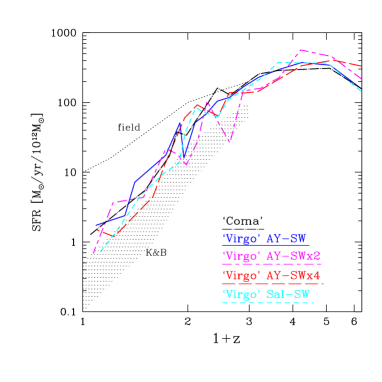
Figure 1: Normalized global star formation rates in the “Virgo” and “Coma” galaxies, excluding the youngest stars (less than 1 Gyr old) in the inner 10 kpc of the cDs; symbols are explained in section 2. Also shown are observed rates for field galaxies (dotted, Madau et al., 1998) and those of galaxies in the inner parts of rich clusters (shaded region, from Kodama & Bower, 2001).

4 Scaling properties of the cluster light

The near-infrared luminosity of galaxies is only negligibly affected by recent star formation activity, thus giving a robust measure of the actual stellar content of a cluster (Kauffmann & Charlot 1998). In Fig. 2 we show the total (2.2$\mu$) K-band luminosity of galaxies within $r_{500}$ versus the total mass inside of $r_{500}$ (which in the $\Lambda$CDM model is approximately half of the virial radius) for individual clusters in the simulated sample — including objects of lower mass than “Virgo” and “Coma”. The various models match quite well the best-fit slope derived observationally by Lin, Mohr & Stanford 2004: $L^{K}_{500}\propto M_{500}^{0.72}$, but the runs with additional pre-heating and those with stronger feedback result in a normalization too low with respect to the observations. As to the Salpeter simulations, the excellent agreement seen in this plot is partly affected by the very blue colours of the galaxies (Fig. 10); in bluer bands, e.g. the B band, these simulations results too bright for their cluster mass (Paper I).

The figure’s insert shows the result of correcting for the excess of young cD stars by neglecting the luminosity contribution of stars in the innermost 40 kpc formed at $z\la 1$ (see Paper III for details); the observational data have been corrected as well by excluding the cluster brightest (usually central) galaxy (BCG). The slope of the relation remains essentially the same, though observationally it steepens slightly to $L^{K}_{500}\propto M_{500}^{0.83}$ (Lin et al. 2004). This indicates that the relative contribution of the cD/BCG to the total cluster light decreases with cluster mass.

The regular trend seen in Fig. 2 over a considerable range of mass suggests that star/galaxy formation in groups and clusters tends to be approximately a scaling process; moreover the slope of the observational relation indicates that smaller groups produce stars at higher efficiency than larger clusters, provided that K-band light well traces stellar mass.

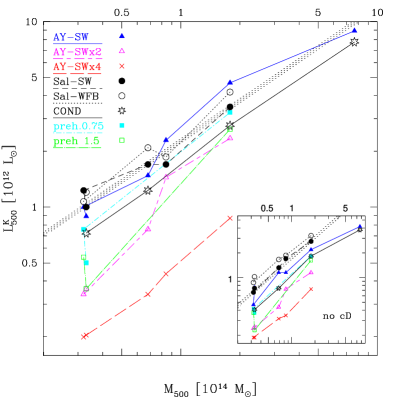
Figure 2: K-band luminosity-mass relation inside of $R_{500}$ at $z$=0 (excluding cD stars in the innermost 10 kpc, younger than 1 Gyr); notice that “Coma” cluster results at $M_{500}\sim 7\times 10^{14}~{}M_{\odot}$ are available only for the AY-SW prescription, with and without thermal conduction (see Table 1). Shaded strip: best-fit relation for a sample of 93 clusters and groups from 2MASS (Lin et al., 2004). In the insert: the same excluding all stars born since $z\simeq 1$ from the central 40 kpc; also the observational best-fit relation has been modified to exclude the BCG.

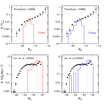
Figure 3: Top panels: B–band luminosity functions at $z$=0 for the standard (AY-SW) “Virgo” (left) and “Coma” (right) simulations; the LFs are normalized to have the same number of galaxies as the observed average LF (Trentham 1998, triangles) within the populated luminosity range ($-19\leq M_{B}\leq-17$). Bottom panels: K–band LFs for the same clusters, compared to the observed average LF by Lin et al. (2004); the dotted line marks the limit $M_{K}\leq-21$ where the observational estimate is considered reliable.

5 The luminosity function of cluster galaxies

In this section we discuss the luminosity function of the population of galaxies in our simulated “Virgo” and “Coma” clusters (excluding the central cDs, which are discussed in Paper III). As mentioned above, we identify for the standard runs 42 galaxies in “Virgo” and 212 galaxies in “Coma”, respectively, with a resolution–limited stellar mass $\ga 2.5\times 10^{9}\,M_{\odot}$, of the order that of the Large Magellanic Cloud. This limit corresponds to $M_{B}\sim-16$ at $z$=0 (Fig. 3).

In Fig. 3 we compare the B–band and K–band luminosity function (LF) of our simulated cluster galaxies, to the observational LFs by Trentham (1998; a weighted mean of 9 low–redshift clusters), and by Lin et al. (2004; a composite LF of 93 clusters and groups from 2MASS data).

For the B–band LF (top panels), the number of resolved individual galaxies quickly drops for objects fainter than $M_{B}\sim-17$, both in “Virgo” and in “Coma”, due to the above mentioned resolution limits and identification procedure. Notice that, although we are missing the dwarf galaxies that largely dominate in number, we are able to describe the bulk of the stellar mass and of the luminosity in clusters, which is dominated by galaxies around $L_{*}$ while dwarfs fainter than $M_{B}\simeq$–17 give a negligible contribution (Cross et al. 2001; Blanton et al. 2004) — though in the simulations, too much of the luminosity and stellar mass expected in objects around $L_{*}$, is instead accumulated in the central cD (see below). Our B–band LF in Fig. 3 is normalized so that, in the luminosity bins that are significantly populated ($-19\leq M_{B}\leq-17$), the overall number of objects is the same as for the observed relative LF (Trentham 1998); in this magnitude range, the shape of the predicted and observed LF is directly comparable. The simulated LF is steeper than the observed one, namely we underestimate the relative number of bright galaxies. One reason for this may be our somewhat biased selection of the group and clusters sample, which consists of fairly relaxed systems, in which no significant merging takes place since $z\la 1$ (see Paper III). This means that most of the massive galaxies have already merged with the central cD by dynamical friction - which is not always the case for real clusters (one likely, nearby example of an unrelaxed cluster is Virgo, e.g., Binggeli et al. 1987).

In the K–band (bottom panels of Fig. 3), our simulated LF reaches fainter magnitudes than the limit $M_{K}<-21$ (dotted line), where the observational LF is considered reliable (Lin et al. 2004). Therefore, we normalize our LF to match the observed number of galaxies within the populated magnitude range and above the resolution limit ($-23.2\leq M_{B}\leq-21$). In the K–band, the lack of massive galaxies in relative number is even more evident.

In Fig. 4 we compare the LFs for the “Virgo” cluster simulated with different IMFs and feedback prescriptions. For the three AY simulations, increasing the feedback strength results in decreasing the masses of all galaxies, and hence, in particular, the number of bright galaxies. The results with thermal conduction (not shown in the figure) are very close to the analogous case without thermal conduction. The LF in the Salpeter case is broader in luminosity, due the lower stellar feedback with respect to the AY IMF, allowing a larger accumulation of stellar mass in galaxies. The trend is even stronger in the Sal-WFB case. Notice that, though the Salpeter IMF simulations are more successful in forming massive galaxies and would thus compare more favourably to the observed LF, this comes at the expense of a too large cold fraction with respect to observations (Table 1 and Paper I). Other reasons to disfavour the Salpeter IMF simulations are the low predicted metallicities in the ICM (Table 1 and Paper I), and the too blue colours of the galaxies (§ 6).

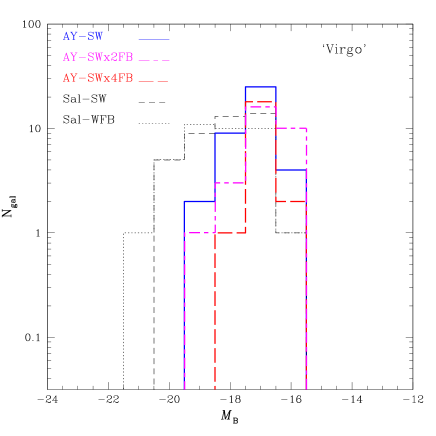
Figure 4: Same as in top panels of Fig. 3 for various “Virgo” simulations; symbols are explained in section 2.

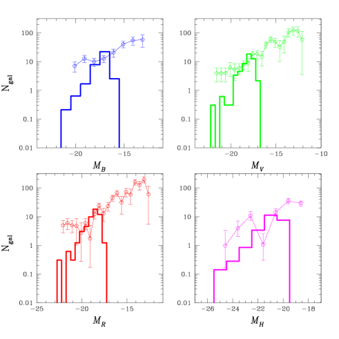
Figure 5: Absolute luminosity functions at $z$=0 of the “Coma” cluster within the relevant projected area (see text) in the B, V, R, H bands, compared with observed Coma LFs from Andreon & Cuillandre 2002 (B, V, R), and Andreon & Pellò 2000 (H).

In Fig. 5 we compare the LF of the “mini-Coma” cluster, in absolute number of galaxies, to the observed Coma LFs: besides discussing the distribution of the stellar mass in the simulations (cD vs. bright galaxies vs. dwarf galaxies) we want to test if the actual number of the galaxies formed in the simulation is sensible. The Coma LF is from Andreon & Cuillandre (2002) and Andreon & Pelló (2000); for the comparison, we compute the luminosity functions of galaxies in our simulated cluster within projected, off-center areas comparable to the areas covered by the observations — about (0.8 Mpc)² in B, (1 Mpc)² in V, R and (0.5 Mpc)² in H. There is quite good agreement with the observed number of galaxies over the luminosity range that is significantly populated by the galaxies identified in the simulation. However, as already noticed from the relative LF in Fig. 3, we are “missing” the bright end tail of the LF, a problem which does not seem to be cured by increased resolution (see §5.1). These results on the absolute LF confirm that the problem is not that we form too few galaxies in the simulations (whence one could statistically “miss” the fewer galaxies at the bright end of the LF), but that in fact there is a lack of bright galaxies in favour of the overgrown cD.

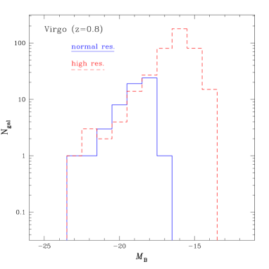
Figure 6: “Absolute” luminosity function of “Virgo” in the B-band, both at normal (solid histogram) and 8 times higher (dashed) resolution, at the epoch $z\simeq 0.8$.

5.1 Resolution effects

In order to test for numerical resolution effects, one simulation of the “Virgo” system with the standard AY-SW model was run at 8 times higher mass and 2 times higher force resolution. At the time of writing, this simulation has reached $z\simeq$0.8, so that in Fig. 6 we can compare the Virgo LF for the two different resolutions at $z\simeq$0.8. As expected, at higher resolution the LF extends to fainter magnitudes. This is due to the higher force and mass resolution, which allows one to resolve as several small (proto-)galaxies an object which was previously initially identified as one large proto-galaxy. However, above the resolution limit for the galaxy identification, the LF appears to be strikingly robust to resolution effects, and consequently so is all the discussion in the previous section. The global stellar content of the cluster is also essentially resolution independent: the total mass of stars at $z\simeq$0.8 inside of the virial radius is $3.0\cdot 10^{12}M_{\odot}$ for the normal resolution case and $3.4\cdot 10^{12}M_{\odot}$ for the high-resolution one. The corresponding masses of stars in galaxies other than the cD are 9.1 and 9.2$\cdot 10^{11}M_{\odot}$; the total masses of stars outside of the cD (adopting $r_{\rm{cD}}$=50 kpc) are 1.7 and 2.0$\cdot 10^{12}M_{\odot}$, and the masses of stars in the cD are 1.3 and 1.4$\cdot 10^{12}M_{\odot}$, respectively. The total numbers of galaxies identified, assuming $N_{min}=$7 in both cases, are 50 and 341, respectively.

In conclusion, at higher resolution more substructure can be identified extending the LF at the dwarf galaxy end; yet the luminosity of the second brightest galaxy (after the cD) in the two simulations of different resolution is quite similar. Moreover, the number of galaxies brighter than $\approx L^{*}$ remains fairly unaffected when going to higher resolution: enhancing resolution does not increase the number of bright cluster galaxies. Analogous results are obtained from another resolution test we performed, on a smaller system (a group of galaxies of virial mass 0.48 $\cdot 10^{14}M_{\odot}$) evolved down to $z=0$: the higher resolution does not affect the luminosity of the second ranked galaxy nor helps increasing the number of bright ($\sim L_{*}$) galaxies. These tests indicate that the lack of bright galaxies in the normal resolution simulations of our ”Virgo” and ”Coma” clusters is not an effect of numerical “over–merging”.

“Classic” semi-analytical models of cluster formation also faced, to some extent, the problem that the cD became too bright and the number of lower ranked, bright galaxies was depleted. Springel et al. (2001) suggested that numerical over–merging onto the central cD in dissipationless dark matter simulations could deplete the number of galaxies at the bright end of the LF, and showed that for semi–analytical models this problem can be significantly improved on by suitable identification of dark matter substructure, or of “haloes within haloes”. This is not a solution in our case, however, because we identify as galaxies all bound systems containing as little as $N_{min}$=7 star particles, and increasing resolution does not increase the number of bright galaxies. Moreover, in hydrodynamical simulations there is as of yet no physical way to quench the central, semi-steady cooling flow; such late gas accretion accounts for part of the excess of the cD masses.

5.2 Redshift evolution of the Luminosity Function

The LF in clusters can evolve due to two effects: passive luminosity evolution from the aging of the stellar populations, and mass evolution due to dynamical effects such as mergers, tidal stripping and dynamical friction. Cluster galaxies are known to consist of old stellar populations, with the bulk of their star formation occurring at $z$$\gg$1. However, they may not have been completely assembled by $z\sim 1$, and they may still undergo one or two significant mergers since then, or grow by gas accretion (van Dokkum et al., 1999).

The observed evolution of the luminosity function is a powerful probe for the assembly epoch of galaxies. From a theoretical point of view, hierarchical models of galaxy formation based on semi–analytical prescriptions tend to predict a deficit of massive galaxies at $z\sim 1$, as a result of the ongoing mass assembly activity at lower redshift (Kauffmann & Charlot, 1998). More recent models, based on a flat $\Lambda$CDM cosmology and with updated star formation, feedback and wind prescriptions perform much better and agree with the observed number of massive galaxies up to $z=1.2-1.5$; however they still face problems with a deficit at higher redshifts as well as with the colours of massive galaxies, underpredicting the number of red early type galaxies and of Extremely Red Objects. In the deep field, the observed evolution seems to lie in between the predictions of current hierarchical models and those of the monolithic, pure luminosity evolution scenario (Somerville et al. 2004; Stanford et al. 2004).

For clusters instead, recent results from the observations of distant objects suggest that the evolution of the LF is best modelled by pure luminosity evolution: Barger et al. (1996, 1998), De Propris et al. (1999), Kodama & Bower (2003) found that, after correcting for this effect and for cosmological dimming, the galaxy mass function has actually evolved little over time; the K–band LF at $z\sim 1$ is consistent with pure luminosity evolution with constant stellar mass and early redshifts of star formation ($z_{f}\ga 2$).

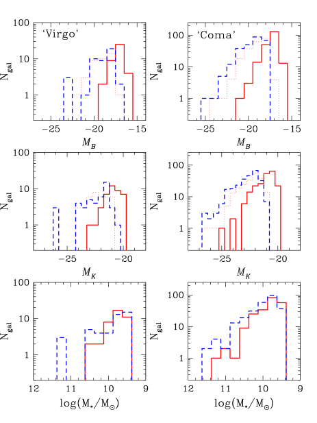
Figure 7: Top panels: Luminosity functions in absolute number of galaxies per B-band magnitude bin for the standard (AY-SW) “Virgo” and “Coma” simulations, at $z=0$ (solid lines) and $z=1$ (dashed lines); the dotted lines represents the expected $z=1$ LF if pure passive evolution of the stellar populations is applied to the $z=0$ LF. Middle panels: Same, for the K-band luminosity functions. Bottom panels: Mass function of cluster galaxies at $z=0$ and $z=1$.

In Fig. 7 we show the evolution of the B and K band LFs of our “Virgo” and “Coma” clusters. We computed the (rest–frame) LF of the galaxies identified in the $z=1$ frame; this is shifted to brighter magnitudes with respect to the distribution at $z=0$, and both luminosity evolution and dynamical mass evolution are seen to play a role in our simulated clusters. In particular, since the bulk of the stars in our galaxies are formed at $z\raisebox{-3.8pt}{$\;\stackrel{{\scriptstyle\textstyle>}}{{\sim}}\;$}2$ (see Paper III and Fig. 9, bottom panel), luminosity dimming is an important effect.

We also computed the LF at $z=1$ as expected from pure passive evolution of the $z=0$ LF, by considering the star particles in each of the galaxies identified at $z=0$, and computing the luminosity they had back at a $\sim$7.5 Gyr younger age. Such “pure passive evolution” LF is displayed as a dotted line in Fig. 7, and it matches quite closely the actual LF in the $z=1$ frame (apart from the absence of a few bright galaxies, see below). This indicates that luminosity dimming of the stellar populations drives most of the LF evolution and the fading to fainter magnitudes from $z=1$ to $z=0$ for the simulated galaxy population; this is in line with the results of Kodama & Bower (2003).

In the brightest luminosity bins of our LF, some additional, dynamical effect seems to be required since more bright galaxies are identified at $z=1$ than expected from pure passive evolution; especially in the case of the “Coma” simulation, where 263 galaxies ar found at $z=1$ versus 212 at $z=0$. To assess mass evolution effects, we plot in the lower panels of Fig. 7 the mass function of (the stellar component of) cluster galaxies at $z=1$ and at $z=0$. The two mass functions are very similar at the low mass end, but a few rather massive objects (above $M_{*}\sim 4\times 10^{10}$ $M_{\odot}$) present at $z=1$ “disappear” at $z=0$. Inspection of the simulations show that these objects have merged with the cD at $z$=0.

As shown in § 5.1, numerical “over–merging” onto the central cD cannot be the main reason for missing galaxies at the bright end of the simulated LF. The lack of bright, massive galaxies other than the cD at $z$=0 is probably largely affected by our group and cluster selection procedure, which picks out extremely relaxed objects at z=0, as discussed in §5. All in all, “Coma” presents a less relaxed structure than “Virgo”, as also inferred by the shapes of the LF at z=0 and z=1. Indeed even for “Virgo” we do see a deficiency of bright galaxies at z=0, but not at z=1, where a gap is just due to poorer statistics of galaxy numbers. Work is in progress however to analyze a large sample of groups more randomly selected (hence including both relaxed and unrelaxed object) to assess the bias induced by the selection procedure (Sommer–Larsen, D’Onghia & Romeo 2005, in preparation).

5.3 Passive evolution and the Fundamental Plane

In the previous section we computed the pure passive evolution dimming, from $z=1$ to $z=0$, corresponding to the cluster galaxies identified at $z=0$. Constraints on the passive evolution of ellipticals in clusters are derived from the observed evolution of the Fundamental Plane (FP), indicating a dimming of about 1.2 magnitudes in the B band in the redshift range $z=1\rightarrow 0$; assuming a Salpeter slope for the IMF, this implies a redshift of formation $z_{for}\geq 2.5$ for the stellar populations (Van Dokkum & Stanford 2003; Wuyts et al. 2004; Renzini 2005; Holden et al. 2005).

A direct comparison to FP constraints is hampered by the fact that in our LF we miss the bright, massive elliptical galaxies defining the observed FP; nevertheless, it is interesting to comment on the predicted passive evolution of our galaxies. In the table below we show the B magnitude evolution $\Delta M_{B}=M_{B}(z=0)-M_{B}(z=1)$ predicted by the SSPs in use, as a function of the assumed redshift of formation $z_{for}$ of the stellar population. These values are largely independent of the SSP metallicity, at least within a factor of 3–4 of the solar value (which is certainly representative of the bright galaxies in our simulations).

$z_{for}$	$\Delta M_{B}$ (Salp)	$\Delta M_{B}$ (AY)
5	0.97	1.07
3	1.15	1.27
2.5	1.26	1.40
1.5	2.01	2.20

Since younger stellar populations dim faster, the lower the redshift of formation, the faster the magnitude evolution between $z=1$ and $z=0$. For the Salpeter IMF, our photometric code predicts that the observed dimming of $\sim$1.2 mag, corresponds to $z_{for}\geq$2.5 in agreement with the above mentioned studies. The rate of dimming depends however also on the slope of the IMF, being faster for shallower IMFs; for an AY slope, the luminosity evolution is in fact slightly faster requiring $z_{for}\geq 3$ (see also Renzini 2005). Taking into account progenitor bias, i.e. the fact the progenitors of the youngest present–day early-type galaxies drop out of the sample at high redshift, the actual magnitude evolution of ellipticals might be underestimated by about 20% (van Dokkum & Franx 2001). In this case, $\Delta M_{B}=1.4$ mag and $z_{for}=2.5$ (AY IMF) are still compatible with observations.

The mean redshift of formation for the stars in our simulated galaxies is  2.5 (Paper III), which is on average compatible with FP constraints but the scatter around the mean is large. Younger star particles, where present, dominate in the luminosity contribution at $z=1$ and induce a much faster overall evolution (cf. a stellar population formed at z=1.5 dims by more than 2 mag). This scatter in age makes some of our galaxies evolve faster than indicated by FP studies.

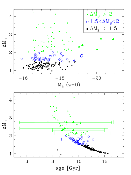
Figure 8: Passive evolution in B magnitude between $z=1$ and $z=0$, predicted for the Coma cluster galaxies. $\Delta M_{B}=M_{B}(z=0)-M_{B}(z=1)$ is plotted as a function of the present–day magnitudes at $z=0$ (top panel) and as a function of age (bottom panel). For the six brightest objects (largw symbols) we also show the internal spread in stellar ages responsible for the very large magnitude evolution (see text).

This is illustrated in Fig. 8, where we show the magnitude evolution $\Delta M_{B}=M_{B}(z=0)-M_{B}(z=1)$ for our simulated “Coma” galaxies as a function of their present–day magnitude and as a function of average stellar age. The age–dimming (i.e., $z_{for}-\Delta M_{B}$) relation is well defined in the bottom panel and the FP constraint of 1.2-1.4 mag is met by objects older than 10.5-11 Gyr. The scatter above the lower envelope of the age–dimming relation is due to internal age scatter within the galaxies. We analyze in particular the six brightest objects in the simulation, with $M_{B}<-19$ (large symbols in the figure), which are more relevant for comparison to the bright spheroidals on the FP. These objects are 9–10 Gyr old (average age), i.e. $z_{for}$=1.5–2 which corresponds to $\Delta M_{B}=1.5-2$. However, they also present a large internal scatter in stellar age, as shown by the errorbars in the bottom panel (stretching from the minimum to the maximum stellar age in each object). In particular, they contain stars as young as 8 Gyr, and some of them have minor tails of SF stretching to $z<1$, i.e. to ages younger than 7.5 Gyr. The presence of these younger–than–average stars has negligible effects on the present–day appearance of these galaxies, since at $z=0$ all the stars are already quite “old” (ages $>5$ Gyr) — see also Fig. 9d showing that the luminosity age equals the actual average age for these objects, while it would be significantly younger if the younger stellar component were prominent. However, back at $z=1$ these younger–than–average stars become very bright, young populations (ages $\leq$1 Gyr) with a major contribution to luminosity, so that they ultimately drive the overall brightening of the galaxy when we trace it back to to $z=1$.

The median of the luminosity evolution for all the Coma galaxy population is 1.4 mag (in agreement with the average $z_{for}=2.5$), i.e. close to the FP constraint; however the large internal age scatter within the galaxies, especially the brighter ones, induces an overall predicted passive evolution for the LF more extreme than that (Fig. 7).

Higher resolution simulations can possibly help with this problem, by both anticipating the overall SF process (resolving smaller, hence denser, substructures) and reducing the internal poissonian noise in the stellar age distribution of the individual galaxies. However, the high resolution test presented in § 5.1 does not show major differences in the LF down to $z=0.8$ (Fig. 6), suggesting that we have reached a resolution good enough to grasp the main galaxy properties. We are probably then facing here a standard problem of hierarchical models of galaxy formation, i.e. that they predict both slightly younger average ages (Fig. 9d) and a larger (internal) age scatter for more massive objects, both trends in contrast with observational evidence (see Section 3 and references therein).

We notice however that the faint end of the present–day colour–magnitude relation of E+S0 cluster galaxies seems to be largely populated by objects which reddened onto the Red Sequence only recently, while at high $z$ they were much bluer; an effect that is usually associated to the spiral $\longrightarrow$ S0 transformation and to the Butcher–Oemler effect from intermediate redshift to $z=0$ (e.g. De Lucia et al. 2004; see also Section 3 and references therein). These objects are certainly not the same probed by the FP at high redshift, which relates to the most massive ellipticals. Also, Holden et al. (2005) find a large scatter in mass–to–light ratio and hence magnitude evolution for the least massive ellipticals selected at high $z$, with masses around $10^{11}~{}M_{\odot}$ (comparable to the most massive objects in our final galaxy population, Fig. 7). Henceforth, it is possible that our simulations miss in fact exactly the massive spheroidals at the bright end of the LF, which are most meaningful for FP constraints. The issue needs then to be revisited once the problem of properly populating the bright end of the LF is solved for simulated clusters.

6 The Red Sequence

The light and stellar mass in clusters of galaxies is dominated by bright, massive ellipticals (Abell 1962, 1965). These are known to form a tight colour-magnitude relation, or Red Sequence (Bower, Lucey & Ellis 1992ab; Gladders et al. 1998; Andreon 2003; Hogg et al. 2004; McIntosh et al. 2005). In Fig. 9ab we compare the colour–magnitude relation for our “Coma” cluster galaxies, excluding the cD, to the observed Red Sequence of Coma from Bower et al. (1992) and Terlevich, Caldwell & Bower (2001), assuming a distance modulus to Coma of 35.1, i.e. $H_{0}\sim$70 km sec^-1 Mpc^-1 (Baum et al. 1997). The slope of the observed Red Sequence is sensitive to aperture effects: fixed–aperture observations are often used, measuring a smaller fraction of the total light in larger objects than in smaller ones; combined with colours gradients, this introduces a bias in the sense of measuring systematically redder colours in larger galaxies, i.e. a steepening of the actual colour–magnitude relation. When the analysis is instead performed on an area that scales with the size of the galaxy, e.g. within the effective radius, or within a given isophotal/photometric radius, the colour–magnitude relation is in fact flatter (Terlevich et al. 2001; Scodeggio 2001; and references therein). For Coma and Virgo, Bower et al. measured colours within a fixed aperture of 11” and 60” respectively, corresponding to a fixed radius of $5h^{-1}\sim 7.15$ kpc. Henceforth for a proper comparison, we computed and plotted in Fig. 9 the colours for our simulated galaxies within a projected radius of 7.15 kpc. The magnitude in abscissa are instead total magnitudes, as adopted by Bower et al.

The solid lines in panels (a,b) indicate the observed slope and location of the Red Sequence; the dotted line is a least square fit to our data. There is overall good agreement, although our Red Sequence is not as extended as the observed one (which reaches magnitudes as bright as $M_{V}=-23$), due to the lack of simulated galaxies at the bright end of the luminosity function discussed in the previous section. Our slope for the (U-V) vs. V relation (Fig. 9a), is slightly flatter than the observed one, but the colours of the three brightest objects are in good agreement with observations, even within the observed small scatter. These objects are the most significant ones if we remember that the observed slope is defined only for $M_{V}<-19$, extended down to $M_{V}<-18$ by Terlevich et al. The slope of the simulated (V-K) vs. V relation (Fig. 9b) is in perfect agreement with the observed one.

Although we formally obtain the right slopes, the simulated Red Sequence also displays a much larger scatter than the observed Coma Red Sequence, which is very narrow down to $M_{V}\sim-18$ (dashed and dotted lines in Fig. 9ab; see also Fig. 2a in Gladders et al., 1998). Such large scatter is partly due to Poissonian noise from the small number of star particles in the low luminosity galaxies. Besides, while the observed colour–magnitude relation refers to early type galaxies (E/S0), we did not attempt any morphological classification and a priori selection of our simulated galaxies due to limited resolution.

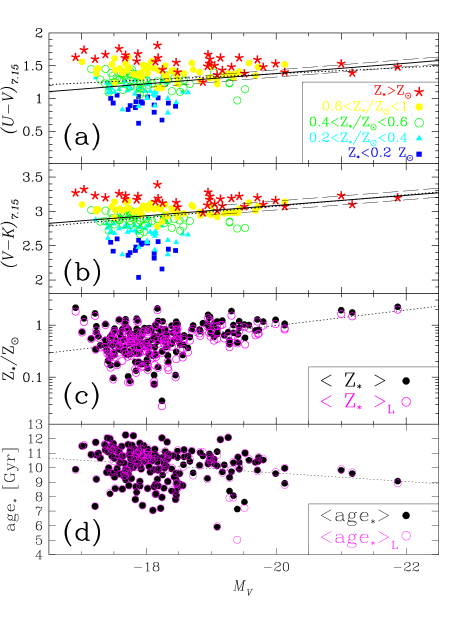
Figure 9: (a–b) Colour–magnitude relation for galaxies in the simulated “Coma” cluster (data points and dotted linear fit line), compared to the observed relation with its scatter (solid and long–dashed lines, from Bower et al. 1992; short–dashed lines, from Terlevich et al. 2001). The extension of the dashed lines indicates the magnitude range probed observationally, while the average fit relation (solid line) has been extrapolated to lower magnitudes. (c) Metallicity–luminosity relation for the “Coma” galaxies (full symbols for mass–averaged stellar metallicity, open symbols for luminosity–weighted metallicity); the dotted line is a linear fit. (d): Age–luminosity relation for the “Coma” galaxies (mass–average and luminosity–weighted stellar ages); the dotted line is a linear fit.

The colour–magnitude relation is classically interpreted as a mass–metallicity relation (Kodama & Arimoto 1997). In our simulations, the bulk of the stars in galaxies are formed at $z\ga$2 (see also Paper III), hence age trends among galaxies are only mild (Fig. 9d) and the colour–magnitude relation is mostly a metallicity effect (Fig. 9c). The metallicity–luminosity relation for our cluster galaxies is displayed Fig. 9c, both in terms of mass-weighted metallicity and of (V–band) luminosity–weighted metallicity. The latter is systematically slightly lower than the actual mass-averaged stellar metallicity, as expected since more metal–poor populations tend to be brighter, skewing the luminosity–weighted metallicity to lower values (Greggio 1997); the trend with galaxy luminosity is however maintained. Although metal-rich objects seem to exist at all luminosities, the fraction of metal–poor galaxies (as well as the scatter in metallicity) increases with decreasing galaxy luminosity; the average stellar metallicity decreases for fainter galaxies (dotted line), which ultimately drives the simulated colour–magnitude relation.

Fig. 9d shows the average stellar ages for the galaxies. All the galaxies consist of old stellar populations, with average ages between 7 and 12 Gyrs. The brighter galaxies ($M_{V}<-20$) are essentially coeval, 9–10 Gyr old. The luminosity–weighted ages are generally very close to the mass averaged ages, which implies a small scatter of stellar ages within the individual galaxies: extended tails or recent episodes of star formation, would strongly skew the luminosity–weighted estimate to younger ages. The scatter in age among the galaxies is around 30%, with a mild trend of decreasing age with increasing luminosity (dotted line), but the effect is much smaller that the systematic variation in metallicity (a factor of 10, Fig. 9c). This confirms that the color–magnitude relation of our simulated galaxies is driven by a mass-metallicity relation, in agreement with common wisdom. The mild age trend, which tends to act in the opposite direction (making fainter galaxies redder) is probably responsible of the fact that our colour-magnitude relation is not as steep as the observed one.

At all magnitudes, even the faintest ones, we find some simulated galaxies with large (super–solar) metallicities. For dwarf ellipticals, a very large spread in metallicities and colours with a tail of red, metal rich objects, is in fact observed but at fainter magnitudes than those probed here ($M_{B}>-15$, Conselice et al. 2003). Metal rich dwarf ellipticals in clusters may possibly originate from larger (and hence more metal rich) galaxies that have suffered considerable tidal stripping in the cluster potential. To test this hypothesis we traced the evolution of the nine galaxies with $Z_{*}>Z_{\odot}$ and $M_{V}>-18$, shown in the top panel of Fig. 8, back in time. Two of the galaxies were found to contain a significantly larger mass of stars at $z\sim 1.5-2.5$ (when these galaxy reach their maximum stellar masses), whereas the stellar masses of the other seven were found not to change much since their ”birth”. Therefore, in our simulations, stripping of originally larger galaxies is one possible, but not predominant, channel to form dwarf galaxies of high metallicity.

In Fig. 10 we assess the dependence of the simulated Red Sequence on the parameters of the simulation, by considering the “Virgo” cluster computed with different physical prescriptions (see Section 2 and Table 1). For all the AY simulations the galaxies scatter about the observed Red Sequence, and their average location in the colour–magnitude diagram appears to be robust with respect to the inclusion of thermal conduction or preheating, and also to enhanced feedback efficiency (AY-SWx2; we do not display the case AY-SWx4 since the total number of galaxies and their average mass are quite small — see Fig. 4 — but they still scatter around the observed line). The scatter is however very large and the magnitude range of the galaxies formed quite limited (missing the bright end of the LF), so that one cannot make meaningful comparisons to the observed slope of the Red Sequence.

Significantly different is the case of the Salpeter IMF simulations. The scatter is much reduced and the slope of the observed colour–magnitude relation is well reproduced; however, the simulated galaxies are offset to the blue of the observed Red Sequence. Let us discuss the latter problem first. In the standard SuperWind case (Sal-SW) in particular, the stellar populations are too metal poor, hence too blue, to match the observed Red Sequence. Notice that the blue colours are not due to younger stellar ages, since the star formation history in the Virgo cluster is very similar for the Salpeter and the AY simulations (Fig. 1). In the weak feedback scenario, where effective supernova energy injection is limited to the early epochs (Sal-WFB) the simulated Red Sequence falls closer to the observed one, though still on the blue side. With minor feedback the galaxies retain a much larger fraction of the metals they produce, thereby the stellar metallicities can grow larger; however, the price is a predicted enrichment of the ICM far below the observed levels for the Sal-WFB simulations (Table 1 and Paper I). Henceforth, top–heavier IMFs than the Salpeter IMF are needed, not only for the sake of the ICM enrichment but also to reproduce the observed colours and metallicities of the stellar populations. In fact the Salpeter IMF does not produce enough metals, and/or locks too much mass in stars, to account for the observed metallicities in the ICM and in cluster galaxies at the same time (Portinari et al. 2004, and Paper I).

As to the increased dispersion in galaxy properties for the AY vs. Salpeter simulations, this is likely induced by the much stronger feedback (a combination of the SW prescription with a top–heavy IMF). As a consequence, the Red Sequence in the AY simulations is much less tight, with no well-defined slope, although the average colours of the galaxies agree with observations much better than in the Salpeter case. If the dispersion is mostly due to numerical effects, because of the small number of particles in the individual galaxies, higher resolution simulations should show a reduced scatter — something to be tested in future work.

In summary, the zero–point of the simulated Red Sequence appears to be a robust prediction of the simulations, quite unaffected by the adopted physical prescriptions other than the chosen IMF, which sets the typical stellar metallicity attainable in cluster galaxies. The observed slope of the colour–magnitude relation is well reproduced in the Salpeter simulations (plagued however by an offset to too blue colours and low metallicities); for the AY simulations the scatter is much larger but the average colours are better reproduced.

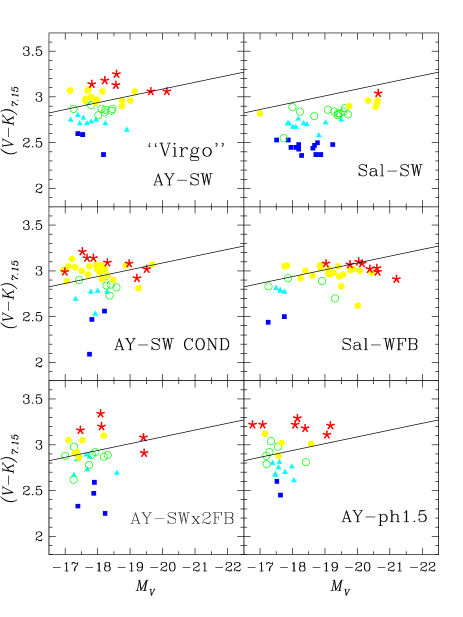
Figure 10: Red Sequence for our simulated “Virgo” cluster with different physical input. AY: Arimoto & Yoshii IMF; Sal: Salpeter IMF; SW: “standard” feedback prescription; SWx2: two times stronger feedback efficiency; WFB: weak feedback (strong feedback active only at early times); COND: thermal conduction included; ph: energy preheating at $z=3$. Symbols follow the metallicity coding of Fig. 9.

7 Conclusions

In this paper we have presented for the first time and analyzed the properties of the galaxy population in clusters, as predicted from full ab initio cosmological + hydrodynamical simulations.

Our results are based on cosmological simulations of galaxy clusters including self-consistently metal-dependent atomic radiative cooling, star formation, supernova and (optionally) AGN driven galactic super-winds, non-instantaneous chemical evolution, effects of a meta-galactic, redshift dependent UV field and thermal conduction. In relation to modelling the properties of cluster galaxies this is an important step forward with respect to previous theoretical works on the subject, e.g. based on semi–analytical recipes super–imposed on N–body only simulations.

The global star formation rates of the “Virgo” and “Coma” cluster galaxies are found to decrease very significantly with time from redshift $z$=2 to 0, in agreement with what is inferred from observations of the inner parts of rich clusters (e.g., Kodama & Bower 2001).

We have determined galaxy luminosity functions for the “Virgo” and “Coma” clusters in the $B,V,R,H$ and $K$ bands; the comparison to observed galaxy luminosity functions reveals a deficiency of bright galaxies ($M_{\rm{B}}$$\la$–20). We carried out a test simulation of “Virgo” at eight times higher mass resolution and two times higher force resolution; the results of this test, still running at the present, indicate that the above mentioned deficiency of bright galaxies is not due to “over–merging”; higher resolution simulations of “Coma” clusters are in progress as well to further check this point. From a suite of simulations for the “Virgo” cluster with different input physics, we find that the deficiency of bright galaxies becomes less prominent with decreasing super-wind strength, in particular for models invoking a Salpeter IMF and only early feedback; in fact more mass can be accumulated in stars and galaxies, with low feedback. Such models, however, present various drawbacks: the cold fraction is too high and the metal production is too low, as seen in the too blue colours of the galaxies and/or in the low metallicity of the ICM, which can hardly be enriched to the observed level of about 1/3 of solar abundance; the latter point is discussed in detail in Paper I, but it also follows from more general arguments (Portinari et al. 2004). The bright galaxy deficiency might be explained as a selection effect, in the sense that we have selected cluster haloes for the TreeSPH re-simulations, which are “too relaxed” compared to an average cluster halo, so that the brightest galaxies have by now merged into the central cD by dynamical friction; we shall return to this in a forthcoming paper.

The redshift evolution of the luminosity functions from redshift $z$=1 to 0 is mainly driven by passive luminosity evolution of the stellar populations, but also by the above mentioned merging of bright galaxies into the cD.

The slope of the colour–magnitude relation of the simulated galaxies is in good agreement with the observed one, however the scatter is larger than observed, partly due to poissoinian noise within the fainter galaxies which are formed by small numbers of star particles. Such internal dispersion in stellar ages is also responsible for a luminosity dimming between $z=1$ and $z=0$, faster than indicated by the observed evolution of the Fundamental Plane. The typical average galaxy colours are best matched when adopting a top-heavy IMF (as originally suggested by Arimoto & Yoshii 1987), while Salpeter IMF simulations yield too blue colours. Moreover we find that the average metallicity of the simulated galaxies increases with luminosity, and that the brightest galaxies are essentially coeval. Hence, the colour–magnitude relation results from metallicity rather than age effects, as concluded by Kodama & Arimoto (1997) on the basis of its observed evolution.

References

- (1) Abell G.O., 1962, IAU Symp. 15, ed. G.C. McVittie (Macmillan Press, New York), p.213
- (2) Abell G.O., 1965, ARA&A 3, 1
- Andreon and Pellò (2000) Andreon S., Pellò R., 2000, A&A 353, 479
- Andreon & Cuillandre (2002) Andreon S., Cuillandre J.C., 2002, ApJ 569, 144
- Andreon (2003) Andreon S., 2003, A&A 409, 37
- Antonuccio et al. (2003) Antonuccio-Delogu V., Becciani U., Ferro D., 2003, Comput. Phys. Commun. 155, 159
- (7) Arimoto N., Yoshii Y., 1987, A&A 173, 23
- (8) Arnaud M., Rothenflug R,, Boulade O., Vigroux L., Vangioni–Flam E., 1992, A&A 254, 49
- (9) Balogh M.L., Pearce F.R., Bower R.G., Kay S.T., 2001, MNRAS 326, 1228
- Barger et al. (1996) Barger A.J., Aragón-Salamanca A., Ellis R.S., Couch W.J., Smail I., Sharples R.M., 1996, MNRAS 279, 1
- Barger et al. (1998) Barger A.J. et al., 1998, ApJ 501, 522
- Baum et al. (1997) Baum W.A., Hammergren M., Thomsen B., Groth E.J., Faber S.M., Grillmair C.J., Ajhar E.A., 1997, AJ 113, 1483 Baumgartner W.H., Loewenstein M., Horner D.J., Mushotzky R.F., 2005, ApJ 620, 680
- (13) Benson A.J., Ellis R.S., Menanteau F., 2002, MNRAS 336, 564
- (14) Benson A.J., Frenk C.S., Baugh C.M., Cole S., Lacey C.G., 2001, MNRAS 327, 1041
- (15) Bernardi M., et al., 2003, AJ 125, 1866
- Binggeli et al. (1987) Binggeli, B., Tammann, G.A., & Sandage, A., 1987, AJ 94, 251
- (17) Binney J., Tabor G., 1995, MNRAS 276, 663
- (18) Blanton M.R., Lupton R.H., Schlegel D.J., Strauss M.A., Brinkmann J., Fukugita M., Loveday J., 2004, ApJ submitted (astro-ph/0410164)
- (19) Bower R.G., 1991, MNRAS 248, 332
- Bower et al. (1992a) Bower R.G., Lucey J.R., Ellis R.S., 1992a, MNRAS 254, 589
- Bower et al. (1992b) Bower R.G., Lucey J.R., Ellis R.S., 1992b, MNRAS 254, 601
- (22) Bressan A., Chiosi C., Tantalo R., 1996, A&A 311, 425
- (23) Butcher H., Oemler A., 1978, ApJ 226, 559
- (24) Butcher H., Oemler A., 1984, ApJ 285, 426
- (25) Carraro G., Chiosi C., Girardi L., Lia C., 2001, MNRAs 327, 69
- (26) Cen R., 2005, ApJ 620, 191
- (27) Chiosi C., Carraro G., 2002, MNRAS 335, 335
- (28) Churazov E., Sunyaev R., Forman W., Böhringer H., 2002, MNRAS 332, 29
- (29) Ciotti L., Ostriker J.P., 2001, ApJ 551, 131
- (30) Cleary P.W., Monaghan J.J., 1999, Jour. Comp. Phys. 148, 227
- Conselice et al. (2003) Conselice C.J., Gallagher J.S., Wyse R.F.G., 2003, AJ 125, 66
- (32) Cowie L.L, McKee C.F., 1977, ApJ 211, 135
- (33) Cross N., et al., 2001, MNRAS 324, 825
- (34) De Grandi S., Ettori S., Longhetti M., Molendi S., 2004, A&A 419, 7
- De Lucia et al. (2004) De Lucia G., Kauffmann G., White S.D.M., 2004, MNRAS 349, 1101
- De Lucia et al. (2004) De Lucia G., et al., 2004, ApJL 610, 77
- De Propris et al. (1999) De Propris R., Stanford S.A., Eisenhardt P.R., Dickinson M., Elston R., 1999, ApJ 118, 719
- (38) Diaferio A., Kauffmann G., Balogh M.L., White S.D.M., Schade D., Ellingson E., 2001, MNRAS 323, 999
- (39) Dressler A., 1980, ApJ 236, 351
- (40) Dressler A., 2004, in Clusters of galaxies: probes of cosmological structure and galaxy evolution, J.S. Mulchaey , A. Dressler and A. Oemler (eds.), Carnegie Observatories Astrophysics Series, vol. 3 (Cambridge: Cambridge Univ. Press), p. 207
- (41) Ellingson E., Lin H., Yee H.K.C., Carlberg R.G., 2001, ApJ 547, 609
- (42) El-Zant A., Kim W.-T., Kamionkowski M., 2004, MNRAS 354, 169
- (43) Fabian A., 1994, ARA&A 32, 277
- (44) Fabian A.C., Voigt L.M., Morris R.G., 2002, MNRAS 335, L71
- (45) Finoguenov A., David L.P., Ponman T.J., 2000, ApJ 544, 188
- (46) Finoguenov A., Arnaud M., David L.P., 2001, ApJ 555, 191
- (47) Fujita Y., Suzuki T.K., Wada K., 2004, ApJ 600, 650
- Girardi et al. (2002) Girardi L., Bertelli G., Bressan A., Chiosi C., Groenewegen M.A.T., Marigo P., Salasnich B., Weiss A., 2002, A&A 391, 195
- Gladders et al. (1998) Gladders M.D., Lopez-Cruz O., Yee H.K.C., Kodama T., 1998, ApJ 501, 571
- (50) Gomez P.L., et al., 2003, ApJ 584, 210
- (51) Goto T., 2005, MNRAS 356, L6
- (52) Goto T., Yamauchi C., Fujita Y., Okamura S., Sekiguchi M., Smail I., Bernardi M., Gomez P.L., 2003, MNRAS 346, 601
- Greggio (1997) Greggio L., 1997, MNRAS 285, 151
- (54) Hogg D.W., et al., 2004, ApJ 601, L29
- (55) Holden B.P. et al., 2005, ApJ 620, L83
- Jubelgas et al. (2004) Jubelgas M., Springel V., Dolag K., 2004, MNRAS 351, 423
- (57) Jørgensen I., Franx M., Hjorth J., van Dokkum P.G., 1999, MNRAS 308, 833
- (58) Kaiser C.R., Binney J., 2003, MNRAS 338, 837
- Kauffmann (1995) Kauffmann G., 1995, MNRAS 274, 153
- Kauffmann & Charlot (1998) Kauffmann G., Charlot S., 1998, MNRAS 297, L23
- Kauffmann et al. (1999) Kauffmann G., Colberg J.M., Diaferio A., White S.D.M., 1999, MNRAS 303, 188
- (62) Knight P.A., Ponman T.J., 1997, MNRAS 289, 955
- Kodama and Arimoto (1997) Kodama T., Arimoto N., 1997, A&A 320, 41
- Kodama and Bower (2001) Kodama T., Bower R.G, 2001, MNRAS 321, 18
- Kodama and Bower (2003) Kodama T., Bower R.G, 2003, MNRAS 346, 1
- (66) Kritsuk A.G., 1996, MNRAS 280, 319
- (67) Lewis G.F., Babul A., Katz N., Quinn T., Hernquist L., Weinberg D.H., 2000, ApJ 526, 623
- (68) Lia C., Portinari L., Carraro G., 2002a, MNRAS 330, 821
- (69) Lia C., Portinari L., Carraro G., 2002b, MNRAS 335, 864
- Lin et al. (2003) Lin Y., Mohr J.J., Stanford S.A., 2003, ApJ 591, 749
- Lin et al. (2004) Lin Y., Mohr J.J., Stanford S.A., ApJ 610, 745
- Madau et al. (1998) Madau P., Pozzetti L., Dickinson M., 1998, ApJ 498, 106
- (73) Makishima K., et al. 2001, PASJ 53, 401
- (74) Margoniner V.E., de Carvalho R.R., Gal R.R., Djorgovski S.G., 2001, ApJ 548, L143
- (75) Matsushita K., Belsole E., Finoguenov A., Böhringer H., 2001, A&A 386, 77
- (76) Matteucci F., Vettolani P., 1988, A&A 202, 21
- (77) McIntosh D.H., Zabludoff A.I., Rix H.-W., Caldwell N., 2005, ApJ 619, 193
- (78) Molendi S., Pizzolato F., 2001, ApJ 560, 194
- (79) Nagai D., Kravtsov A.V., 2004, in Outskirts of galaxy clusters: intense life in the suburbs, IAU Coll. 195, eds. A. Diaferio et al., p. 296
- (80) Narayan R., Medvedev M.V., 2001, ApJ 562, L129
- (81) Peterson J.R., Paerels F.B.S., Kaastra J.S., Arnaud M., Reiprich T.H., Fabian A.C., Mushotzky R.F., Jernigan J.G., Sakelliou I., 2001, A&A 365, L104
- (82) Peterson J.R., Kahn, S.M., Paerels F.B.S., Kaastra J.S., Tamura T., Bleeker J.A.M., Ferrigno C., Jernigan J.G., 2003, ApJ 590, 207
- (83) Poggianti B.M., Smail I., Dressler A., Couch W.J., Barger A.J., Butcher H., Ellis R.S., Oemler A., 1999, ApJ 518, 576
- (84) Poggianti B.M., Bridges T.J., Komiyama Y., Yagi M., Carted D., Mobasher B., Okamura S., Kashilawa N., 2004, ApJ 601, 197
- Portinari et al. (2004) Portinari L., Moretti A., Chiosi C., Sommer-Larsen J., 2004, ApJ 604, 579
- Renzini (2003) Renzini A., 2004, in Clusters of galaxies: probes of cosmological structure and galaxy evolution, J.S. Mulchaey, A. Dressler and A. Oemler (eds.), Carnegie Observatories Astrophysics Series, vol. 3 (Cambridge: Cambridge Univ. Press),p. 261
- Renzini (2005) Renzini A., 2005, in IMF@50: the Initial Mass Function 50 years later, E. Corbelli, F. Palla and H. Zinnecker (eds.), Astrophysics and Space Science Library (Dordrecht: Kluwer Academic Publishers), in press (astro-ph/0410295)
- (88) Renzini A., Ciotti L., D’Ercole A., Pellegrini S., 1993, ApJ 419, 52
- Romeo et al. (2004) Romeo A.D., Sommer-Larsen J., Portinari L., Antonuccio V., 2004, in preparation (Paper I)
- (90) Salpeter E.E., 1955, ApJ 121, 161
- (91) Scodeggio M., 2001, AJ 121, 2413
- (92) Smith G.P., Treu T., Ellis R.S., Moran S.M., Dressler A., 2005, ApJ 620, 78
- (93) Somerville R., et al., 2004, ApJ 600, L135
- Sommer-Larsen (2004) Sommer-Larsen J., 2004, in Proceedings of the Vulcano conference on ”Modelling the intergalactic and intracluster media”, V. Antonuccio et al. (eds.), to be published online on MemSAIt - Supplementi.
- Sommer-Larsen et al. (2003) Sommer-Larsen J., Götz M., Portinari L., 2003, ApJ 596, 47
- Sommer-Larsen et al. (2004) Sommer-Larsen J., Romeo A.D., Portinari L., 2005, MNRAS 357, 478 (Paper III).
- Springel and Hernquist (2002) Springel V., Hernquist L., 2002, MNRAS 333, 649
- Springel et al. (2001) Springel V., White S.D.M., Tormen G., Kauffmann G., 2001, MNRAS 328, 726
- (99) Stanford S.A., Dickinson M., Postman M., Ferguson H.C., Lucas R.A., Conselice C.J., Budavári T., Somerville R., 2004, AJ 127, 131
- (100) Suginohara T., Ostriker J.P., 1998, ApJ 507, 16
- (101) Sutherland R.S., Dopita M.A., 1993, ApJS 88, 253
- (102) Tamura T., et al. 2001, A&A 365, L87 5J.R., 2004, A&A 420, 135
- Terlevich et al. (2002) Terlevich A.I., Caldwell N., Bower R.G., 2001, MNRAS 326, 1547
- Tornatore et al. (2003) Tornatore L., Borgani S., Springel V., Matteucci F., Menci N., Murante G., 2003, MNRAS 342, 1025
- Tornatore et al. (2004) Tornatore L., Borgani S., Matteucci F., Recchi S., Tozzi P., 2004, MNRAS 349, L19
- (106) Trager S.C., Faber S.M., Worthey G., Gonzales J.J., 2000, AJ 120, 165
- Trentham (1998) Trentham N., 1998, MNRAS 295, 360
- (108) Treu T., et al., 2005, ApJ submitted (astro-ph/0503164)
- Valdarnini (2003) Valdarnini R., 2003, MNRAS 339, 1117
- (110) van Dokkum P.G., Stanford S.A., 2003, ApJ 585, 78
- (111) van Dokkum P.G., Franx M., 2001, ApJ 553, 90
- van Dokkum et al. (1999) van Dokkum P.G., Franx M., Fabricant D., Kelson D.D., Illingworth G.D., 1999, ApJ 520, L95
- van Dokkum et al. (2001) van Dokkum P.G., Stanford S.A., Holden B.P., Eisenhardt P.R., Dickinson M., Elston R., 2001, ApJ 552, L101
- (114) Voit G.M., 2004, Rev. Mod. Phys. in press (astro-ph/0410173)
- Voit et al. (2003) Voit G.M., Balogh M.L., Bower R.G., Lacey C.G., Bryan G.L., 2003, ApJ 593, 272
- (116) Wuyts S., van Dokkum P.G., Kelson D.D., Franx M., Illingworth G.D., 2004, ApJ 605, 677