Brane universes tested by supernovae Ia

Abstract

We discuss observational constrains coming from supernovae Ia imposed on the behaviour of the Randall-Sundrum models. In the case of dust matter on the brane, the difference between the best-fit Perlmutter model with a $\Lambda$-term and the best-fit brane models becomes detectable for redshifts $z>1.2$. It is interesting that brane models predict brighter galaxies for such redshifts which is in agreement with the measurement of the $z=1.7$ supernova. We also demonstrate that the fit to supernovae data can also be obtained, if we admit the ”super-negative” dark energy (phantom matter) $p=-(4/3)\varrho$ on the brane, where the dark energy in a way mimics the influence of the cosmological constant. It also appears that the dark energy enlarges the age of the universe which is demanded in cosmology. Finally, we propose to check for dark radiation and brane tension by the application of the angular diameter of galaxies minimum value test. We point out the existence of coincidence problem for the brane tension parameter.

I Introduction

In recent several years a lot of effort has been done on the idea that our Universe is a boundary of a higher-dimensional spase time manifold Arkani-Hamed98 ; Arkani-Hamed99 . Kaluza and Klein first discussed $5-dimensional$ space time to unify a gravity and electromagnetism. Among supersting theories which may unify all interactions M-theory is a strong candidate for the description of real world. In this theory, gravity is a truly higher-dimensional theory, becoming effectively 4-dimensional at lower energies. The standard model matter fields are confined to the 3-brane while gravity can, by its universal character, propagate in all extra dimensions. In the brane world models inspired by string/M theory (rs1 ,rs2 , hw ) new two parameters which doesn’t present in standard cosmology are introduced, namely brane tension $\lambda$ and dark radiation $U$. One of new approaches was proposed by Randall and Sundrum rs1 , rs2 where our Minkowski brane is localized in 5dimensional anti-de Sitter space time with metric:

$$ds^{2}=\exp(-2|y|l)(-dt^{2}+d\vec{x}^{2})+dy^{2}.$$ (1)

For $y\neq 0$, this metric satisfies the 5dimensional Einstein equation with the negative cosmological constant $\tilde{\check{\Lambda_{(5)}}}\propto-l^{-2}$. The brane is located at $y=0$ and the induced metric on brane is a Minkowski metric. The bulk is a 5-dimensional anti-deSitter metric with $y=0$ as a boundary.

We should mention that before the Randall and Sundrum work rs2 where they proposed a mechanism to solve the hierarchy problem by a small extra dimension, large extra dimensions were proposed to solve this problem by Arkani-Hamed et.al. Arkani-Hamed98 ; Arkani-Hamed99 . This gives an interesting feature because TeV gravity might be realistic and quantum gravity effects could be observed by a next generation particle collider. The Newtonian gravity potential on the brane is recovered at lowest order $V(r)=\frac{GM}{r}(1+\frac{2l^{2}}{3r^{2}})$. In this paper we demonstrate that if the brane world is the Randall-Sundrum version is realistic we may find some evidence of higher dimensions.

In Szydlo02 we gave the formalism to express dynamical equations in terms of dimensionless observational density parameters $\Omega$. In this notation (see also Dabrowski96 ; AJI+II ; AJIII ) the Friedmann equation for brane universes takes the form

$$\frac{1}{a^{2}}\left(\frac{da}{dt}\right)^{2}=\frac{C_{\gamma}}{a^{3\gamma}}+\frac{C_{\lambda}}{a^{6\gamma}}-\frac{k}{a^{2}}+\frac{\Lambda_{(4)}}{3}+\frac{C_{\cal U}}{a^{4}},$$ (2)

where $a(t)$ is the scale factor, $k=0,\pm 1$ the curvature index, here we use natural system of units in which $8\pi G=c=1$, $\Lambda_{(4)}$ is the 4-dimensional cosmological contant, and $\gamma$ the barotropic index ($p=(\gamma-1)\varrho$, $p$ - the pressure, $\varrho$ - the energy density), the constants $C_{\lambda}=1/6\lambda\cdot a^{6\gamma}\varrho^{2}$ and $C_{\cal U}=2/\lambda\cdot a^{4}{\cal U}$, $C_{\lambda}$ comes as a contribution from brane tension $\lambda$, and $C_{\cal U}$ as a contribution from dark radiation.

Because $\rho^{2}$ term and dark radiation term do not appear in the standard cosmology, such terms could provide a smal window to see the extra dimensions.

In order to study observational tests we now define dimensionless observational density parameters

$$\Omega_{\gamma} = \frac{1}{3H^{2}}\varrho,\hskip 15.0pt\Omega_{\lambda}=\frac{1}{6H^{2}\lambda}\varrho^{2},\hskip 15.0pt\Omega_{\cal U}=\frac{2}{H^{2}\lambda}{\cal U},$$

$$\Omega_{k} = -\frac{k}{H^{2}a^{2}},\hskip 15.0pt\Omega_{\Lambda_{(4)}}=\frac{\Lambda_{(4)}}{3H^{2}},$$ (3)

where the Hubble parameter $H=\dot{a}/a$, and the deceleration parameter $q=-\ddot{a}a/\dot{a}^{2}$ , so that the Friedmann equation (2) can be written down in the form

$$\Omega_{\gamma}+\Omega_{\lambda}+\Omega_{k}+\Omega_{\Lambda_{(4)}}+\Omega_{\cal U}=1.$$ (4)

Note that $\Omega_{\cal U}$ in (I), despite standard radiation term, can either be positive or negative.

It is useful to rewrite (2) to the dimensionless form. Let us consider a standard Friedmann-Robertson-Walker universe (hereafter FRW) filled with mixture of matter with the equation of state $p_{i}=(\gamma_{i}-1)\rho_{i}$. Then we obtain the basic equation in the form:

$$\frac{\dot{x}^{2}}{2}=\frac{1}{2}\Omega_{k,0}+\frac{1}{2}\sum_{i}\Omega_{i,0}x^{2-3\gamma_{i}}=-V(x)\\$$ (5)

$$\ddot{x}=-\frac{1}{2}\sum_{i}\Omega_{i,0}(2-3\gamma_{i})x^{1-3\gamma_{i}}=-\frac{\partial V(x)}{\partial x}$$ (6)

where $i=(\gamma,\lambda,\Lambda,U)$, and

$$x\equiv\frac{a}{a_{0}},\qquad T\equiv|H_{0}|t,\qquad\dot{}\equiv\frac{d}{dT}.$$ (7)

and $t$ is original cosmological time, $V$ is the potential function.

Therefore the dynamics of the considered model is equivalent to introducing fictitious fluids which mimic $\rho^{2}$ contribution and dark energy term. For dark energy $\gamma=4/3$ whereas for brane $\gamma_{\lambda}=2\gamma$. The presented formalism is useful in analysis of observational tests of brane models.

Above relations allow to write down an explicit redshift-magnitude relation for the brane models to study their compatibility with astronomical data which is the subject of the present paper. Obviously, the luminosity of galaxies depends on the present densities of the different components of matter content $\Omega_{i}$ given by (I) and their equations of state, reflected by the value of the barotropic index $\gamma_{i}$.

II Brane cosmologies and SNIa observations

Let us consider an observer located at $r=0$ at the moment $t=t_{0}$ which receives a light ray emitted at $t=t_{1}$ from the source of the absolute luminosity $L$ located at the radial distance $r_{1}$. The redshift $z$ of the source is related to the scale factor $a(t)$ at the two moments of evolution by $1+z=a(t_{0})/a(t_{1})\equiv a_{0}/a$. If the apparent luminosity of the source as measured by the observer is $l$, then the luminosity distance $d_{L}$ of the source is defined by the relation

$$l={L\over 4\pi d_{L}^{2}},$$ (8)

where

$$d_{L}=(1+z)a_{0}r_{1}\equiv\frac{{\cal D}_{L}(z)}{H_{0}},$$ (9)

and ${\cal D}_{L}$ is the dimensionless luminosity distance. The observed and absolute luminosities are defined in terms of K-corrected apparent and absolute magnitudes $m$ and $M$. When written in terms of $m$ and $M$, Eq. (8) yields

$$m(z)={\cal M}+5\log_{10}[{\cal D}_{L}(z)],$$ (10)

where ${\cal M}=M-5\log_{10}H_{0}+25$. For homogeneous and isotropic Friedmann models one gets

$${\cal D}_{L}(z)=\frac{\left(1+z\right)}{\sqrt{{\cal K}}}S(\chi)$$ (11)

where $S(\chi)=\sin\chi$ with ${\cal K}=-\Omega_{k,0}$ when $\Omega_{k,0}<0$; $S(\chi)=\chi$ with ${\cal K}=1$ when $\Omega_{k,0}=0$; $S(\chi)=\sinh\chi$ with ${\cal K}=\Omega_{k,0}$ when $\Omega_{k,0}>0$. From the Friedmann equation (2) and the form of the FRW metric we have

$$\chi(z)=\sqrt{{\cal K}}\int\limits_{0}^{z}\left\{\Omega_{\lambda,0}\left(1+z^{{}^{\prime}}\right)^{6\gamma}+\Omega_{\gamma,0}\left(1+z^{{}^{\prime}}\right)^{3\gamma}\right.$$

$$\left.+\Omega_{k,0}\left(1+z^{{}^{\prime}}\right)^{2}+\Omega_{{\cal U},0}\left(1+z^{{}^{\prime}}\right)^{4}+\Omega_{\Lambda_{(4),0}}\right\}^{-1/2}dz^{{}^{\prime}}.$$ (12)

Firstly, we will study the case $\gamma=1$ (dust on the brane; we will label $\Omega_{\gamma}$ by $\Omega_{m}$). The case $\gamma=2/3$ (cosmic strings on the brane) has recently been studied in Singh1/3 where, in fact, $\Omega_{\cal U}$ and $\Omega_{\lambda}$ were neglected and where the term $\Omega_{m,0}(1+z^{{}^{\prime}})^{3}$ was introduced in order to admit dust matter on the brane. This case was already presented in a different framework in Ref. AJIII . Secondly, we will study the case $\gamma=-1/3$ (dark energy on the brane darkenergy - we will label this type of matter with $\Omega_{d}$ instead of $\Omega_{\gamma}$).

Now we test brane models using the Perlmutter samples Perlmutter99 . In order to avoid any possible selection effects, we use the full sample (usually, one excludes two data points as outliers and another two points, presumably reddened, from the full sample of 60 supernovae). It means that our basic sample is the Perlmutter sample A Perlmutter99 . We test our model using the likelihood method Riess98 .

First of all, we estimate the value of $\mathcal{M}$ from the full sample of 60 supernovae. For the flat model we obtained $\mathcal{M}=-3.39$ which is in agreement with the results of Efstathiou99 ; Vishwakarma . Also, we obtained for the Perlmutter model the same value of $\chi^{2}=96.5$ what is in agreement with Perlmutter99 .

Neglecting dark radiation $\Omega_{{\cal U},0}=0$ we formally got the best fit ($\chi^{2}=94.6$) for $\Omega_{k,0}=-0.9$, $\Omega_{m,0}=0.59$, $\Omega_{\lambda,0}=0.04$, $\Omega_{\Lambda,0}=1.27$, (see Tab I) which is completely unrealistic Peebles02 ; Lahav02 , because $\Omega_{m,0}=0.59$ is too large in comparison with the observational limit (also $\Omega_{k,0}=-0.9$ is not very realistic from the observational point of view).

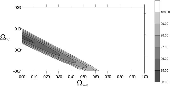
Figure 1: The plot of $\chi^{2}$ levels for flat ($\Omega_{k,0}=0$) brane models with respect to the values of $\Omega_{m,0}$ (horizontal axis) and $\Omega_{\lambda,0}$ (vertical axis).

However, we should note that, in fact, we have an ellipsoid of admissible models in a 3dimensional parameter space $\Omega_{m,0}$, $\Omega_{\lambda,0}$, $\Omega_{\Lambda_{(4)},0}$ at hand. Then, we have more freedom than in the case of analysis of Perlmutter99 where they had only an ellipse in a 2dimensional parameter space $\Omega_{m,0}$, $\Omega_{\Lambda_{(4)},0}$. For a flat model $\Omega_{k,0}=0$ we obtain ”corridors” of possible models (Fig.1). Formally, the best-fit flat model is $\Omega_{m,0}=0.01$, $\Omega_{\lambda,0}=0.09$ $\chi^{2}=94.7$ which is again unrealistic. In the realistic case we obtain for a flat model $\Omega_{m,0}=0.25$, $\Omega_{\lambda,0}=0.02$, $\Omega_{\Lambda_{(4)},0}=0.73$ with $\chi^{2}=95.6$. One should note that all realistic brane models also require the presence of the positive 4-dimensional cosmological constant ($\Omega_{\Lambda_{(4)},0}\sim 0.7$).

There is a question if we could fit a model with negative $\Omega_{\lambda,0}$? For instance, in a flat Universe we could fit the model with $\Omega_{m,0}=0.35$ (too much in comparison with the observational limits on the mass of the cluster of galaxies) $\Omega_{\lambda,0}=-0.01$, $\Omega_{\Lambda,0}=0.66$ ($\chi^{2}=96.3$).

Fig. 2 illustrates the confidence level as a function of ($\Omega_{\mathrm{m},0}$, $\Omega_{\lambda,0}$) for the flat model ($\Omega_{k,0}=0$) minimalized over $\mathcal{M}$ with $\Omega_{\Lambda,0}=1-\Omega_{\mathrm{m},0}-\Omega_{k,0}-\Omega_{\lambda,0}$. In present cases we formally assumed that both positive and negative value of $\Omega_{\lambda,0}$ are mathematically possible. We show that the preferred intervals for $\Omega_{m,0}$ and $\Omega_{\lambda,0}$ are $\Omega_{m,0}<0.4$ and $\Omega_{\lambda,0}>0$.

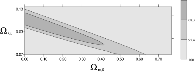
Figure 2: Confidence levels on the plane $(\Omega_{\mathrm{m},0},\Omega_{\lambda,0})$ minimalized over $\mathcal{M}$ for the flat model, and with $\Omega_{\Lambda,0}=1-\Omega_{\mathrm{m},0}-\Omega_{k,0}-\Omega_{\lambda,0}$. The figure shows the ellipses of the preferred value of $\Omega_{\mathrm{m},0}$ and $\Omega_{\Lambda,0}$.

Figure 3: The redshift-magnitude relation for $\gamma=1$ brane universes (dust on the brane). The top line is the best-fit Perlmutter model. with $\Omega_{m,0}=0.28$, $\Omega_{\Lambda_{(4)},0}=0.72$. The bottom line is a flat model with $\Omega_{m,0}=1$. Between these two lines there are brane models with $\Omega_{\lambda,0}\neq 0$: lower–the best-fit nonflat model; higher–the best-fit flat model.

Table 1: Results of the statistical analysis for the dust matter on the brane for Perlmutter Sample A, B, C. Two upper line for each sample are best fit model and best fit flat model for sample. Third line is ”realistic” model with $\Omega_{\text{m},0}\simeq 0.3$. We also include, for sample A the model with $\Omega_{\lambda,0}<0$

Sample	N	$\Omega_{k,0}$	$\Omega_{\lambda,0}$	$\Omega_{m,0}$	$\Omega_{\Lambda,0}$	$\chi^{2}$
A	60	-0.9	0.04	0.59	1.27	94.7
		0.0	0.09	0.01	0.90	94.7
		0.0	0.02	0.25	0.73	95.6
		0.0	-0.01	0.35	0.66	96.3
B	56	-0.1	0.06	0.17	0.87	57.3
		0.0	0.06	0.12	0.82	57.3
		0.0	0.02	0.25	0.73	57.6
C	54	0.0	0.04	0.21	0.73	53.5
		0.0	0.04	0.21	0.73	53.5
		0.0	0.02	0.27	0.71	53.6

In Fig. 3 we present plots of redshift-magnitude relations against the supernovae data. One can observe that in both cases (best-fit and best-fit flat models) the difference between brane models and a pure flat (Einstein-de Sitter) model with $\Omega_{\Lambda_{(4)},0}=0$ is largest for $0.6<z<0.7$ while it significantly decreases for the higher redshifts. It gives us a possibility to discriminate between the Perlmutter model and brane models when the data from high-redshift supernovae is available. On the other hand, the difference between the best-fit Perlmutter model with a $\Lambda$-term Perlmutter99 and the best-fit brane models becomes detectable for redshifts $z>1.2$. It is interesting that brane models predict brighter galaxies for such redshifts which is in agreement with the measurement of the $z=1.7$ supernova Riess01 . In other words, if the farthest $z>1$ supernovae were brighter, the brane universes is allowed.

One should note that we made our analysis without excluding any supernovae from the sample. However, from the formal point of view, when we analyze the full sample A, all models should be rejected even on the confidence level of 0.99. One of the reason could be the fact that the assumed error are too small. However, in majority of papers another solution is suggested. Usually, one excludes 2 supernovae as outliers, and 2 as reddened from the sample of 42 high-redshift supernovae and eventually 2 outliers from the sample of 18 low-redshift supernovae. We decided to use the full sample A as our basic sample because a rejection of any supernovae from the sample can be the source of lack of control for selection effects. However, for completness, we also made our analysis using samples B and C. It emerged that it does not significantly changes our results, though, increases quality of the fit. Formally, the best fit for the sample B (56 supernovae) is ($\chi^{2}=57.3$): $\Omega_{k,0}=-0.1$ $\Omega_{m,0}=0.17$, $\Omega_{\lambda,0}=0.06$, $\Omega_{\Lambda_{(4)},0}=0.87$. For the flat model we obtain ($\chi^{2}=57.3$): $\Omega_{m,0}=0.12$, $\Omega_{\lambda,0}=0.06$, $\Omega_{\Lambda_{(4)},0}=0.82$, while for a ”realistic” model ($\Omega_{m,0}=0.25$, $\Omega_{\lambda,0}=0.02$) $\chi^{2}=57.6$. Formally, the best fit for the sample C (54 supernovae) ($\chi^{2}=53.5$) gives $\Omega_{k,0}=0$ (flat) $\Omega_{m,0}=0.21$, $\Omega_{\lambda,0}=0.04$, $\Omega_{\Lambda_{(4)},0}=0.75$, while for ”realistic” model ($\Omega_{m,0}=0.27$, $\Omega_{\lambda,0}=0.02$) $\chi^{2}=53.6$.

One should note that we have also separately estimated the value of ${\cal M}$ for sample B and C. We obtained ${\cal M}=-3.42$ which is again in a good agreement with the results of Efstathiou99 (for a ”combined” sample one obtains ${\cal M}=-3.45$). However, if we use this value in our analysis it does not change significantly the results ($\chi^{2}$ does not change more than $1$ which is a marginal effect for $\chi^{2}$ distribution for 53 or 55 degrees of freedom).

Figure 4: The redshift-magnitude relation for $\gamma=-1/3$ brane universes (phantom matter on the brane). The top line is the Perlmutter model and the bottom line is the Einstein-de Sitter model. In the middle are two overlapping line for the best-fitted and best-fitted flat brane models.

In Fig. 4 we present a redshift-magnitude relation (II) for brane models with dark energy ($\gamma=-1/3$) and $\Omega_{\cal U}>0$. To obtain an acceptable fit $\Omega_{{\cal U},0}$ should be so large as $\simeq 0.2$. Note that the theoretical curves are very close to that of the Perlmutter model Perlmutter99 which means that the dark energy cancels the positive-pressure influence of the $\varrho^{2}$ term and can simulate the negative-pressure influence of the cosmological constant to cause cosmic acceleration. From the formal point of view the best fit (Tab.II) is ($\chi^{2}=95.4$) for $\Omega_{k,0}=0.2$, $\Omega_{d,0}=0.7$, $\Omega_{\lambda,0}=-0.1$, $\Omega_{{\cal U},0}=0.2$, $\Omega_{\Lambda_{(4)},0}=0$ which means that the cosmological constant must necessarily vanish. From this result we can conclude that the dark energy $p=-(4/3)\varrho$ can mimic the contribution from the $\Lambda_{(4)}$-term in standard models. For the best-fit flat model ($\Omega_{k,0}=0$) we have ($\chi^{2}=95.4$): $\Omega_{d,0}=0.2$, $\Omega_{\lambda,0}=-0.1$, $\Omega_{{\cal U},0}=0.2$, $\Omega_{\Lambda_{(4)},0}=0.7$.

However if we excluded possibility that $\Omega_{\lambda,0}<0$, than for value of the parameter $\Omega_{\lambda,0}=0.01$ we obtain: $\Omega_{k,0}=0.2$, $\Omega_{d,0}=0.5$, $\Omega_{\lambda,0}=0.01$, $\Omega_{{\cal U},0}=0.2$, $\Omega_{\Lambda_{(4)},0}=0,09$ For the best-fit flat model ($\Omega_{k,0}=0$) we have ($\chi^{2}=95.5$): $\Omega_{d,0}=0.05$, $\Omega_{\lambda,0}=0.01$, $\Omega_{{\cal U},0}=0.2$, $\Omega_{\Lambda_{(4)},0}=0,74$ which means that the cosmological constant is not vanish in such type of model.

Table 2: Results of the statistical analysis for the dark energy (phantom matter) on the brane for Perlmutter Sample A with $\Omega_{{\cal U},0}=0.2$ Two upper line are best fit model and best fit flat model for sample. The next two line are the model with $\Omega_{\lambda,0}=0.01$

Sample	N	$\Omega_{k,0}$	$\Omega_{\lambda,0}$	$\Omega_{d,0}$	$\Omega_{\Lambda,0}$	$\chi^{2}$
A	60	0.2	-0.10	0.70	0.00	95.4
		0.0	-0.10	0.20	0.70	95.4
		0.2	0.01	0.50	0.09	95.5
		0.0	0.01	0.05	0.74	96.5

Figure 5: The age of the universe $t_{0}$ in units of $H_{0}^{-1}$ for the brane models with dust ($0\leq\Omega_{m,0}\leq 1$ on the horizontal axis). Here $\Omega_{{\cal U},0}=\Omega_{k,0}=0$, $\Omega_{{\lambda},0}=0,0.05,0.1$ (top, middle, bottom).

III Other tests for brane cosmology

III.1 Brane models and age of the universe

Now let us briefly discuss the effect of brane parameters and dark energy onto the age of the universe which according to (2) is given by

$$H_{0}t_{0}=\int_{0}^{1}\left\{\Omega_{\gamma,0}x^{-3\gamma+4}+\Omega_{{\lambda},0}x^{-6\gamma+4}\right.$$

$$\left.+\Omega_{{\cal U},0}+\Omega_{k,0}x^{2}+\Omega_{\Lambda_{(4)},0}x^{4}\right\}^{-\frac{1}{2}}xdx,$$ (13)

where $x=a/a_{0}$. We made a plot for the dust $\gamma=1$ on the brane in Fig. 5 which shows that the effect of quadratic in energy density term represented by $\Omega_{\lambda}$ is to lower significantly the age of the universe. The problem can be avoided, if we accept the dark energy $\gamma=-1/3$ on the brane darkenergy , since the dark energy has a very strong influence to increase the age. In Fig. 6 we made a plot for this case which shows how the dark energy enlarges the age.

Figure 6: The age of the universe $t_{0}$ in units of $H_{0}^{-1}$ for the brane models with dark energy (phantom matter) on the brane ($0\leq\Omega_{d,0}\leq 1$ on the horizontal axis). Here $\Omega_{{\cal U},0}=0.2$, $\Omega_{{\lambda},0}=0.05,0$ (top, bottom) which shows weaker influence of the brane effects to increase the age.

III.2 Angular diameter versus redshift for brane models

Finally, let us study the angular diameter test for brane universes. The angular diameter of a galaxy is defined by

$$\theta=\frac{d(z+1)^{2}}{d_{L}},$$ (14)

where $d$ is a linear size of the galaxy. In a flat dust ($\gamma=1$) universe the angular diameter $\theta$ has the minimum value $z_{min}=5/4$. It is particularly interesting to notice that for flat brane models with $\Omega_{\lambda,0}\approx 0,\Omega_{\Lambda_{(4)}}\approx 0$ the dark radiation shift the minimum of $\theta(z)$ relation towards to higher $z$ for $\Omega_{{\cal U},0}\leq 0$ while the ordinary radiation shift this minimum towards to lower $z$. It should be also noted that dark radiation decrease the value of $\theta(z_{min})$ for $\Omega_{{\cal U},0}\leq 0$ while the ordinary radiation increase this value. This is a general influence of negative dark radiation onto the angular diameter size for brane models.

Figure 7: The angular diameter $\theta(z)$ for $\Omega_{\lambda,0}=0.1,\Omega_{m,0}=0.3,\Omega_{\Lambda_{(4)}}=0.72$, and the two values of $\Omega_{{\cal U},0}=0.1,-0.1$ (top, middle) in comparison with the model of Perlmutter with $\Omega_{m,0}=0.28,\Omega_{\Lambda_{(4)}}=0.72$ (bottom).

More detailed analytic and numerical studies $\theta(z)$ relation Dabreg02 show that the increase of $z_{min}$ is even more sensitive to negative values of $\Omega_{\lambda,0}$ ($\varrho^{2}$ contribution). Similarly as for the dark radiation $\Omega_{{\cal U},0}$, the minimum disappears for some large negative $\Omega_{{\lambda},0}$. Positive $\Omega_{{\cal U},0}$ and $\Omega_{{\lambda},0}$ make $z_{min}$ decrease. In Fig. 7 we present a plot from which one can see the sensitivity of $z_{min}$ to $\Omega_{{\cal U},0}$. We have also checked Dabreg02 that the dark energy $\Omega_{d,0}$ (phantom matter) has very little influence onto the value of $z_{min}$.

IV Conclusions

We shown that there exists an effective method of constraining exotic physics coming from superstrings M theory from observation of distant supernovae. We obtain the estimated value the density parameters $\Omega_{\lambda,0}$ and $\Omega_{\Lambda,0}$ .

Finally, as a result we also obtain that at high redshifts the expected luminosity of supernovae Ia should be brighter then in the Perlmutter model. For the best fit value we obtain $\Omega_{\lambda,0}\simeq 0.01$ which seems to be unrealistic. It is because if we consider pure Randall-Sundrum models, then there is a constraint on the parameter $\Omega_{\lambda,0}$ from the requirement of not violating the four-dimensional gravity on sufficiently large spatial scale. This constraint is that value of $\lambda$ is to be no less than about $(100\,GeV)^{4}$, which means that during the late epoch the $\rho^{2}$ term in the model should be small.

So, the obtained value of $\Omega_{\lambda,0}\sim 0.01$ is the observational limit which is not based on theoretical model assumptions. The density $\rho_{m,0}$ at the time relevant for supernovae measurements is about $(10^{-3}eV)^{4}$. Thus, the size of the parameter $\Omega_{\lambda,0}$ is on purely theoretical grounds, at most $10^{-56}$. The fits discussed in the paper innvolve $\Omega_{\lambda,0}$ of order $0.01$. Therefore similarly to the cosmological constant problem there is a coincidence problem with brane tension $\lambda$ (it is treated as a constant) namely: why don’t we see the large brane tension expected from the Randall-Sundrum theory which is about $10^{54}$ times larger than the value predicted by the Friedmann equation which fit SNIa data. A phenomenological solution to this problem seems to be dynamically decaying $\lambda$.

V Acknowledgements

The author are very grateful Prof M.Da̧browski for his comments and interesting remarks.

References

- (1) N. Arkani-Hamed, S. Dimopoulos, G. Dvali, Phys. Lett. B (1998) 429, 263
- (2) N. Arkani-Hamed, S. Dimopoulos, G. Dvali, Phys. Rev. D (1999) 59, 086004
- (3) L. Randall and R. Sundrum, Phys. Rev. Lett., 83 (1999), 3370
- (4) L. Randall and R. Sundrum, Phys. Rev. Lett., 83 (1999), 4690.
- (5) P. Hořava and E. Witten, Nucl. Phys. B460 (1996), 506; ibid B475, 94.
- (6) M. Szydłowski, M.P. Da̧browski, and A. Krawiec, Phys. Rev. D66 (2002), 064003 (hep-th/0201066).
- (7) M.P. Da̧browski, Ann. Phys (N. Y.) 248 (1996) 199.
- (8) M.P. Da̧browski and J. Stelmach, Astron. Journ. 92 (1986), 1272; ibid 93 (1987), 1373.
- (9) M.P. Da̧browski and J. Stelmach, Astron. Journ. 97 (1989), 978.
- (10) P. Singh, R.G. Vishwakarma and N. Dadhich, hep-th/0206193.
- (11) R.R. Caldwell, astro-ph/9908168, S. Hannestad and E. Mörstell, astro-ph/0205096, P.H. Frampton, astro-ph/0209037.
- (12) S. Perlmutter et al., Ap. J. 517, (1999) 565.
- (13) A. G. Riess et al. Astron. J. 116 (1998) 1009.
- (14) G. Efstathiou, Mon. Not. R. Astr. Soc. 303 (1999), 147.
- (15) G. R. Vishwakarma, Gen. Rel. Grav. 33 (2001), 1973.
- (16) P. J. E. Peebles, B. Ratra Rev. Mod. Phys 75 (2003), 559 astro-ph/0207347
- (17) O. Lahav 2002 astro-ph/0208297
- (18) A.G. Riess et al., Ap. J. 560 (2001), 49.
- (19) M.P. Da̧browski, W. Godłowski, and M. Szydłowski, in preparation.