Iron abundances from high-resolution spectroscopy of the open clusters NGC 2506, NGC 6134, and IC 4651

This is the first of a series of papers devoted to derive the metallicity of old open clusters in order to study the time evolution of the chemical abundance gradient in the Galactic disk. We present detailed iron abundances from high resolution ($R\;\lower 2.58334pt\hbox{$\sim$}\kern-7.75pt\raise 2.79857pt\hbox{$>$}\;40,000$) spectra of several red clump and bright giant stars in the open clusters IC 4651, NGC 2506 and NGC 6134. We observed 4 stars of NGC 2506, 3 stars of NGC 6134, and 5 stars of IC 4651 with the FEROS spectrograph at the ESO 1.5 m telescope; moreover, 3 other stars of NGC 6134 were observed with the UVES spectrograph on Kueyen (VLT UT2). After excluding the cool giants near the red giant branch tip (one in IC 4651 and one in NGC 2506), we found overall [Fe/H] values of $-0.20\pm 0.01$, $rms$ = 0.02 dex (2 stars) for NGC 2506, $+0.15\pm 0.03$, $rms$ = 0.07 dex (6 stars) for NGC 6134, and $+0.11\pm 0.01$, $rms$ = 0.01 dex (4 stars) for IC 4651. The metal abundances derived from line analysis for each star were extensively checked using spectrum synthesis of about 30 to 40 Fe I lines and 6 Fe II lines. Our spectroscopic temperatures provide reddening values in good agreement with literature data for these clusters, strengthening the reliability of the adopted temperature and metallicity scale. Also, gravities from the Fe equilibrium of ionization agree quite well with expectations based on cluster distance moduli and evolutionary masses.

1 Introduction

Our understanding of the chemical evolution of the Galaxy has tremendously improved in the last decade, thanks to the efforts and the achievements both on the observational and on the theoretical sides. Good chemical evolution models nowadays can satisfactorily reproduce the major observed features in the Milky Way. There are, however, several open questions which still need to be answered.

One of the important longstanding questions concerns the evolution of the chemical abundance gradients in the Galactic disk. The distribution of heavy elements with Galactocentric distance, as derived from young objects like HII regions or B stars, shows a steep negative gradient in the disk of the Galaxy and of other well studied spirals.

Does this slope change with time or not ? And, in case, does it flatten or steepen ?

Galactic chemical evolution models do not provide a consistent answer: even those that are able to reproduce equally well the largest set of observational constraints predict different scenarios for early epochs. By comparing with each other the most representative models of the time, Tosi (1996) showed that the predictions on the gradient evolution range from a slope initially positive which then becomes negative and steepens with time, to a slope initially negative which remains roughly constant, to a slope initially negative and steep which gradually flattens with time (see also Tosi 2000 for updated discussion and references).

From the observational point of view, the situation is not much clearer. Data on field stars are inconclusive, due to the large uncertainties affecting the older, metal poorer ones. Planetary nebulae (PNe) are better indicator, thanks to their brightness. PNe of type II, whose progenitors are on average 2–3 Gyr old, provide information on the Galactic gradient at that epoch and show gradients similar to those derived from HII regions. However, the precise slope of the radial abundance distribution, and therefore its possible variation with time is still subject of debate. In fact, the PNe data of Pasquali & Perinotto (1993), Maciel & Chiappini (1994) and Maciel & Köppen (1994) showed gradient slopes slightly flatter than those derived from HII regions, but Maciel, Costa & Uchida (2003) have recently inferred, from a larger and updated PNe data set, a flattening of the oxygen gradient slope during the last 5–9 Gyr.

Open clusters (OC’s) probably represent the best tool to understand whether and how the gradient slope changes with time, since they have formed at all epochs and their ages, distances and metallicities are more safely derivable than for field stars. However, also the data on open clusters available so far are inconclusive, as shown by Bragaglia et al. (2000) using the compilation of ages, distances and metallicities listed by Friel (1995). By dividing her clusters in four age bins, we find in fact no significant variation in the gradient slope, but we do not know if this reflects the actual situation or the inhomogeneities in the data treatment of clusters taken from different literature sources. Inhomogeneity may lead, indeed, to large uncertainties not only on the derived values of the examined quantities, but also on their ranking. Past efforts to improve the homogeneity in the derivation of abundances, distances or ages of a large sample of OC’s include e.g., the valuable works by Twarog et al. (1997) and Carraro et al. (1998), but in both cases they had to rely on literature data of uneven quality. The next necessary step is to collect data acquired and analyzed in a homogeneous way.

For this reason, we are undertaking a long term project of accurate photometry and high resolution spectroscopy to derive homogeneously ages, distances, reddening and element abundances in open clusters of various ages and galactic locations and eventually infer from them the gradient evolution. Age, distance, and reddening are obtained deriving the colour-magnitude diagrams (CMDs) from deep, accurate photometry and applying to them the synthetic CMD method by Tosi et al. (1991). Accurate chemical abundances are obtained from high resolution spectroscopy, applying to all clusters the same method of analysis and the same metallicity scale.

Up to now we have acquired the photometry of 25 clusters and published the results for 14 of them (see Bragaglia et al. 2004 and references therein, Kalirai & Tosi 2004). We have also obtained spectra for about 15 OC’s, and have already obtained preliminary results for a few of them. Complete spectroscopic abundance analysis has been published so far only for NGC 6819 (Bragaglia et al. 2001).

In this paper we present our results for three OC’s, namely NGC 2506, NGC 6134, and IC 4651. Observational data are presented in Section 2, while Section 3 is devoted to the derivation of atmospheric parameters, equivalent widths and iron abundances. A check of the validity of our temperature scale is derived from comparison with reddening estimates from photometry in Section 4. Spectral synthesis for all stars and its importance to confirm the validity of our findings is discussed in Section 5. Finally, Sections 6 and 7 present a comparison with literature determinations, and a summary.

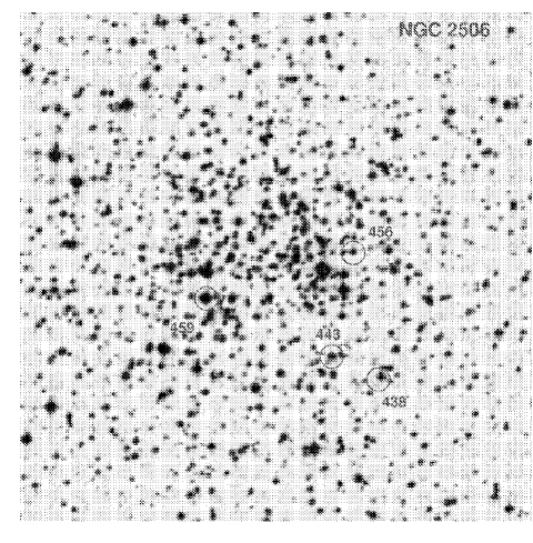
Figure 1: Field of 10 $\times$ 10 arcmin² centered on NGC 2506, with the 4 stars observed with FEROS indicated by their numbers according to Marconi et al. (1997)

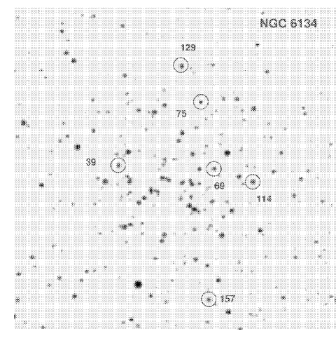
Figure 2: Field of 10 $\times$ 10 arcmin² centered on NGC 6134, with the 6 stars observed with FEROS or UVES indicated by their numbers according to Lindoff (1972).

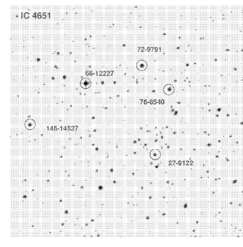
Figure 3: Field of 10 $\times$ 10 arcmin² centered on IC 4651, with the 5 stars observed with FEROS indicated by their numbers according to Lindoff (1972), and Meibom (2000).

2 Observations

Stars were selected on the basis of their evolutionary phases derived from the photometric data. We mainly targeted Red Clump stars (i.e. stars in the core Helium burning phase) because, among the evolved population, they are the most homogeneous group, and their temperatures are in general high enough that, even at the high metallicity expected for open clusters, model atmospheres can well reproduce the real atmospheres (this seems to be not strictly valid for stars near the Red Giant Branch - RGB - tip). We considered only objects for which membership information was available (except for one object in NGC 6134, which however turned out to be member a posteriori), from astrometry (NGC 2506, Chiu & van Altena 1981), and/or radial velocity (NGC 2506: Friel & Janes 1993, Minniti 1995; NGC 6134: Clariá & Mermilliod 1992; IC 4651: Mermilliod et al. 1995).

The three clusters were mainly observed with the spectrograph FEROS (Fiber-fed Extended Range Optical Spectrograph) mounted at the 1.5m telescope in La Silla (Chile) from April 28 to May 1 2000. FEROS is bench mounted, and fed by two fibers (object + sky, entrance aperture of 2.7 arcsec). The resolving power is 48000 and the wavelength range is $\lambda\lambda$ 370-860 nm. There is the possibility of reducing the data at the telescope using the dedicated on-line data reduction package in the MIDAS environment, so we could immediately obtain wavelength calibrated spectra. Multiple exposures for the same star were summed.

Three additional stars in NGC 6134 were observed in July 2000 with UVES (UV-Visual Echelle Spectrograph) on Unit 2 of the VLT ESO-Paranal telescope, as a backup during the execution of another programme (169.D-0473). These data were acquired using the dichroic beamsplitter #2, with the CD2 centered at 420 nm (spectral coverage $\lambda\lambda$ 356-484 nm) and the CD4 centered at 750 nm ($\lambda\lambda$ 555-946 nm). The slit length was 8 arcsec, and the slit width 1 arcsec (resolution of 43000 at the order centers). The UVES data were reduced with the standard pipeline which produces extracted, wavelength calibrated, and merged spectra.

Finding charts for all observed targets are in Figure 1, Figure 2 and Figure 3. The evolutionary status of observed stars is indicated by their position in the CMD, as shown in Figure 4.

Table 1 gives a log of the observations, and more information on the selected stars is listed in Table 2, where values of the S/N are measured at about 670 nm (for multiple exposures, these values refer to the final, co-added spectra).

Table 1: Log of the observations. ID is taken from Marconi et al. (1997) for NGC 2506, from Bruntt et al. (1999) for NGC 6134, and from Lindoff (1972) for IC 4651. ID_BDA is the identification number used in the BDA (Mermilliod 1995). Coordinates are at J2000, and exposure time is in seconds. F indicates FEROS spectra, and U indicates UVES spectra. The P values given for the stars in NGC 2506 are membership probabilities.

ID	IDBDA	Ra	Dec	Date obs.	UT	Exptime	Notes
NGC 2506
459	2122	8:00:05.84	-10:47:13.33	2000-04-28	00:43:04	3600	F, P=0.90
438	3359	7:59:51.79	-10:48:46.51	2000-04-28	01:51:57	3600	F, P=0.94
				2000-04-29	00:02:56	3600	F
443	3231	7:59:55.77	-10:48:22.73	2000-04-29	01:06:30	3600	F, P=0.91
				2000-04-29	02:12:58	3600	F
456	3271	7:59:54.06	-10:46:19.50	2000-04-30	00:56:38	3600	F, P=0.94
				2000-04-30	02:00:05	2400	F
				2000-05-01	01:34:51	2700	F
NGC 6134
404	114	16:27:32.10	-49:09:02.00	2000-04-30	08:04:09	2700	F
				2000-04-30	08:55:42	3229	F
929	39	16:27:57.68	-49:08:36.20	2000-05-01	07:45:47	1800	F
				2000-05-01	08:18:58	1800	F
875	157	16:27:40.05	-49:12:42.20	2000-05-01	08:56:11	2400	F
				2000-05-01	09:39:14	2400	F
428	75	16:27:42.27	-49:06:36.10	2002-07-18	01:25:11	2400	U
421	129	16:27:46.07	-49:05:29.60	2002-07-19	23:36:34	1800	U
527	69	16:27:39.49	-49:08:39.30	2002-07-20	00:09:57	1800	U
IC 4651
27	9122	17:24:50.13	-49:56:55.89	2000-04-28	08:05:27	1800	F
76	8540	17:24:46.78	-49:54:06.94	2000-04-28	08:39:43	1800	F
72	9791	17:24:54.22	-49:53:07.58	2000-04-28	09:15:05	1200	F
56	12227	17:25:09.02	-49:53:57.21	2000-04-28	09:39:59	600	F
146	14527	17:25:23.63	-49:55:47.11	2000-04-29	09:25:29	1500	F
				2000-04-29	09:54:04	1500	F

Table 2: Data for the observed stars in NGC 2506, NGC 6134, and IC 4651. V, B-V are: CCD magnitudes from Marconi et al. (1997) for NGC 2506; photoelectric measurements from Clariá & Mermilliod (1992) for NGC 6134; photoelectric measurements from Eggen (1971), Lindoff (1972), and Jennens & Helfer (1975), as reported in the BDA, for IC 4651. K is taken from 2MASS (Cutri et al. 2003). Stromgren y, b-y are: from Bruntt et al. (1999) for NGC 6134, and Anthony-Twarog & Twarog (2000) for IC 4651. S/N has been measured at about 670 nm. Radial velocities (column 8, in km s^-1), are heliocentric.

ID	V	B-V	K	y	b-y	S/N	RV	Phase
NGC 2506
459	11.696	1.100	9.036	-	-	110	+81.62 $\pm 0.6$	RGBtip
438	13.234	0.944	10.910	-	-	85	+84.64 $\pm 0.3$	clump
443	13.105	0.952	10.791	-	-	77	+84.66 $\pm 0.2$	clump
456	13.977	0.919	11.654	-	-	35	+83.68 $\pm 0.3$	RGB
NGC 6134
404	12.077	1.310	8.819	12.072	0.841	80	$-$24.94 $\pm 0.6$	clump
929	12.202	1.273	9.042	12.197	0.811	56	$-$25.34 $\pm 0.3$	clump
875	12.272	1.268	9.071	12.251	0.820	80	$-$25.26 $\pm 0.2$	clump
428	12.394	1.284	9.208	12.384	0.820	200	$-$26.34 $\pm 0.3$	clump
421	12.269	1.314	8.996	12.245	0.838	200	$-$25.46 $\pm 0.3$	clump
527	-	-	9.189	12.359	0.811	200	$-$25.19 $\pm 0.3$	clump
IC 4651
27	10.91	1.20	-	10.896	0.749	100	$-$30.17 $\pm 0.6$	clump
76	10.91	1.15	-	10.915	0.708	100	$-$29.86 $\pm 0.3$	clump
72	10.44	1.32	-	10.371	0.801	100	$-$30.82 $\pm 0.2$	RGB
56	8.97	1.62	4.660	8.899	1.064	100	$-$29.56 $\pm 0.3$	RGBtip
146	10.94	1.14	8.340	10.923	0.702	100	$-$27.88 $\pm 0.4$	clump

3 Atmospheric parameters and iron abundances

Figure 4: CMD’s for the three clusters, with the stars analyzed here indicated by larger symbols. (a) NGC 2506: B and V taken from Marconi et al. (1997); only stars with membership probability greater than 0.7 (Chiu & van Altena 1981), are shown. (b) NGC 6134: V, b-y taken from Bruntt et al. (1999). (c) IC 4651: V, b-y taken from Anthony-Twarog & Twarog (2000).

3.1 Atmospheric parameters

We derived effective temperatures from our spectra, by minimizing the slope of the abundances from neutral Fe I lines with respect to the excitation potential. The gravities ($\log g$) were derived from the iron ionization equilibrium; to this purpose, we adjusted the gravity value for each star in order to obtain an abundance from singly ionized lines of iron 0.05 dex lower than the abundance from neutral lines. This was done to take into account the same difference between Fe II and F I in the reference analysis made using the solar model from the Kurucz (1995) grid, with overshooting: the present adopted values are $\log n$(Fe)=7.54 for neutral iron and 7.49 for singly ionized iron.

As usual, the overall model metallicity [A/H] was chosen as that of the model atmosphere (extracted from the grid of ATLAS models with the overshooting option switched on) that best reproduces the measured equivalent widths ($EW$’s).

Finally, we determined the microturbulent velocities assuming a relation between $\log g$ and $v_{t}$. This was found to give more stable values than simply adopting individual values of $v_{t}$ by eliminating trends in the abundances of Fe I with expected line strengths. In fact, we found that the star-to-star scatter in Fe abundances was reduced by adopting such a relationship.

Our adopted atmospheric parameters for the three clusters are listed in Table 3.

Table 3: Adopted atmospheric parameters and derived Iron abundances for observed stars in NGC 2506, NGC 6134, and IC 4651; n indicated the number of lines retained in the analysis. In the last column we give for comparison the value of gravity derived from photometric information.

Star	Teff	$\log$ $g$	[A/H]	$v_{t}$	n	[Fe/H]I	$rms$	n	[Fe/H]II	$rms$	$\log\leavevmode\nobreak\ g$
	(K)	(dex)	(dex)	(km s-1)							(phot.)
NGC 2506
459	4450	1.06	$-$0.37	1.36	137	$-$0.37	0.16	10	$-$0.37	0.17	1.74
438	5030	2.53	$-$0.19	1.17	109	$-$0.18	0.11	13	$-$0.18	0.15	2.68
443	4980	2.32	$-$0.21	1.20	102	$-$0.21	0.12	13	$-$0.21	0.09	2.60
456	4970	2.54	$-$0.21	1.17	83	$-$0.21	0.19	10	$-$0.21	0.14	2.95
NGC 6134
404	4940	2.74	+0.11	1.14	128	+0.11	0.16	12	+0.11	0.12	2.60
929	4980	2.52	+0.24	1.17	117	+0.24	0.16	11	+0.24	0.19	2.67
875	5050	2.92	+0.16	1.12	126	+0.16	0.14	13	+0.16	0.15	2.73
428	5000	3.10	+0.22	1.10	82	+0.22	0.16	9	+0.23	0.14	2.76
421	4950	2.83	+0.11	1.13	81	+0.11	0.12	9	+0.11	0.13	2.68
527	5000	2.98	+0.05	1.11	83	+0.05	0.11	8	+0.05	0.12	2.71
IC 4651
27	4610	2.52	+0.10	1.17	128	+0.10	0.15	10	+0.10	0.17	2.51
76	4620	2.26	+0.11	1.21	129	+0.10	0.17	11	+0.10	0.17	2.51
72	4500	2.23	+0.13	1.21	120	+0.13	0.13	9	+0.13	0.21	2.25
56	3950	0.29	$-$0.34	1.46	89	$-$0.34	0.17	6	$-$0.35	0.15	1.23
146	4730	2.14	+0.10	1.21	125	+0.11	0.16	11	+0.11	0.16	2.59

3.2 Equivalent widths

We measured the $EW$’s on the spectra employing an updated version of the spectrum analysis package developed in Padova and partially described in Bragaglia et al. (2001) and Carretta et al. (2002). Measurements of Fe lines were restricted to the spectral range 5500-7000 Å to minimize problems of line crowding and difficult continuum tracing blueward of this region, and of contamination by telluric lines and possible fringing effects redward.

At these high metallicities and cool temperatures, continuum tracing is a major source of uncertainty at the resolution of our spectra, hence we chose to use an iterative procedure. For all clusters, the fraction of the 200 spectral points centered on each line to be measured and used to derive the local continuum level was first set to $1/4$. Following an extensive comparison with spectrum synthesis of Fe I and Fe II lines (see below), we found that the abundances for the stars in NGC 2506 and NGC 6134 (from FEROS spectra) were much too large. This was explained by a too high continuum tracing in these spectra; for these two sets of data we finally adopted $1/2$ as the fraction of spectral points to be used in the estimate of the local continuum. With this new parameters, we performed again the automatic measurements of $EW$’s. Then, the procedure strictly followed that described in Bragaglia et al. (2001).

We used stars in the same evolutionary phase (in this case, clump stars) to obtain an empirical estimate of internal errors in the $EW$’s. We performed the cross-comparisons of the sets of $EW$’s measured for clump stars: 3 stars in IC 4651, 2 in NGC 2506 and 6 in NGC 6134 (in the latter case we treated separately the 3 stars observed with FEROS and the 3 from UVES). Assuming that errors can be equally attributed to both stars in the couple under consideration, we obtain typical errors in $EW$’s of 2.5 mÅ for clump stars in IC 4651, 2.7 mÅ in NGC 2506, 3.6 mÅ and 3.1 mÅ in NGC 6134 (FEROS and UVES spectra, respectively).

The classical formula by Cayrel (1989) predicts that, given the full width half-maximum and the typical $S/N$ ratios (see Table 2) of our spectra, the expected errors are 1.5, 1.8, 2.1 and 0.8 mÅ, respectively, in the four cases.

The comparison with the observed errors shows that another source of error (quadratic sum) has to be taken into account. This is likely to be uncertainties in the positioning of the continuum, an ingredient neglected in Cayrel’s formula. If we consider for simplicity’s sake lines of triangular shape and the relationship between FWHM and central depth used by our automatic procedure, we can estimate that the residual discrepancy can be well explained by errors in the automatic continuum tracing at a level of 1% for clump stars in all clusters.

Sources of oscillator strengths and atomic parameters are the same of Gratton et al. (2003) and discussion and references are given in that paper.

3.2.1 Estimate of errors in atmospheric parameters

Errors in effective temperatures:

Uncertainties in the adopted spectroscopic temperatures can be evaluated from the errors in the slope of the relationship between abundances of Fe I and excitation potentials of the lines. Varying by a given amount the effective temperature, these errors allow us to estimate a standard error of $88\pm 9$, $rms=29$ K (from 11 stars, excluding stars at the RGB tip). Hence, we adopt a standard error of about 90 K, corresponding to an average $rms$ of 0.018 dex/eV in the slope.

This error ($\sigma^{2}_{\rm tot}=\sigma^{2}_{\rm rand.}+\sigma^{2}_{\rm syst.}$) for each individual star includes two contributions:

• a random term $\sigma^{2}_{\rm rand.}$, reflecting the various sources of errors (Poisson statistics, read-out noise, dark current) of spectra, that affects the measurements of the $EW$

• a term $\sigma^{2}_{\rm syst.}$ due to a number of effects that are systematic for each given line (e.g. the presence of blends, of possible features not well accounted for in the spectral regions used to determine the continuum level, the line oscillator strength, etc.)

The first appears as a star-to-star scatter both in the slope abundance/excitation potential and in the error associated to this slope. Analogously, the second contribution shows up as a systematic uncertainty both in the slope and in the associated error. In order to estimate the true random internal error in the derived temperatures, this systematic contribution has to be estimated and subtracted.

We proceed in the following way. Let $j$ be the index associated to the stars and N the number of stars; let $i$ be the index associated to the lines and $M_{j}$ the total number of lines of neutral iron used in the $j-$th star. We then have that the average variance of the distribution of the abundances from individual lines for each star is:

$$\sigma^{2}_{\rm tot}=\frac{\sum_{j}{\left[\frac{\sum_{i}{(x_{ij}-\bar{x}_{j})^{2}}}{M_{j}-1}\right]}}{N}$$

and as an estimate of the systematic contribution we may take:

$$\sigma^{2}_{\rm syst}=\frac{\sum_{i}{\left[\frac{\sum_{j}{(x_{ij}-\bar{x}_{j})^{2}}}{Nj-1}\right]}}{M}$$

In our case, if we exclude from the computations the two tip stars and star 456 in NGC 2506 (the one with lower S/N), we obtain that $\sigma_{\rm tot}=0.141$ dex and $\sigma_{\rm syst.}=0.110$ dex. Thus the truly random contribution to the standard deviation is (quadratic sum) 0.088 dex, hence the fraction of the standard deviation due to star-to-star errors is 0.088/0.141= 0.624. Hence, we may expect that the internal, random error in the temperatures is actually $\sim 55$ K, to be compared with the observed value as derived from independent methods (see below).

Errors in surface gravities:

Since our derivation of atmospheric parameters is fully spectroscopic, a source of internal error in the adopted gravity comes from the total uncertainty in T_eff.

To evaluate the sensitivity of the derived abundances to variations in the adopted atmospheric parameters for Fe (reported in Table 4), we re-iterated the analysis of the clump star 146 of IC 4651 while varying each time only one of the parameters of the amount corresponding to the typical error, as estimated above. Considering the variation in the ionization equilibrium given by a change of 90 K, $\partial$A/$\partial$T${}_{\rm eff}=0.143$ dex, and by a change of 0.2 dex, $\partial$A/$\partial g=0.096$ dex, an error of 90 K in temperatures translates into a contribution of 0.298 dex of error in gravity.

From the above discussion, the contribution due to the random error in temperature and to the error in gravities is then of 0.18 dex.

A second contribution is due to the errors in the measurements of individual lines. If we assume as the error from a single line the average $rms$ of the abundances from Fe I lines (0.14 dex, considering the same stars as above), again we must take into account only the random contribution, 0.088 dex, as estimated above. Weighting this contribution by the average number of measured line (n=111 for Fe I and 12 for Fe II) we obtain a random error of 0.03 dex for the difference between the abundance from Fe II and Fe I lines. This corresponds to another 0.06 dex of uncertainty in $\log g$, to be added in quadrature to the previous 0.18 dex. The total random internal uncertainty in the adopted gravity (quadratic sum) is then 0.20 dex that compares well with the estimate derived from the method described in the following.

Errors in microturbulent velocities:

To estimate the proper error bars in the microturbulent velocity values, we started from the original atmospheric parameters adopted for the clump star 146 in IC 4651. In this star the slope of the line strength $vs$ abundance relation has the same value of the quadratic mean of errors in the slope of all stars, Hence it may be considered as a typical error. The same set of Fe lines was used to repeat the analysis changing $v_{t}$  until the 1$\sigma$ value from the slope of the abundance/line strength relation was reached. A simple comparison allows us to give an estimate of 1$\sigma$ errors associated to $v_{t}$: they are about 0.1 km s^-1, thanks to the large number of used lines of different strengths. Since we estimated that random errors are about 62% of the error budget, the random internal error is then 0.06 km s^-1.

In order to estimate the total error, we have to recall that our final $v_{t}$ values are derived using a relationship between gravities and microturbulent velocities from the former full spectroscopic analysis: $v_{t}=1.5-0.13\times\log g$. The $rms$ scatter around this relationship is 0.17 km s^-1, so that the final error bar in microturbulent velocities derived through the relation is 0.16 km s^-1, which includes a (small) component due to errors in gravity and another component of physical scatter intrinsic to the different stars.

Col. 7 of Table 4 allows to estimate the effect of errors in the $EW$; this was obtained by weighting the average error from a single line with the square root of the mean number of lines (listed in Col. 6 of the Table) measured for each element.

Notice that Cols. 2 to 5 in Table 4 are only meant to evaluate the sensitivity of the abundances to changes in the adopted atmospheric parameters. As discussed above, the actual random errors involved in the present analysis are, more reasonably, 50 K in T_eff, 0.2 dex in $\log g$, 0.05 dex in [A/H] and 0.16 km s^-1 in the microturbulent velocity. Moreover, the sensitivities in Cols. 2 to 5 of this Table are computed assuming a zero covariance between the effects of errors in the atmospheric parameters. In principle, this assumption is not strictly valid, since there are correlations between different parameters: (i) effective temperature and gravities are strictly correlated, so that for each 90 K change in T_eff there is a corresponding change of $\sim 0.3$ dex in $\log g$, since gravities are derived from the ionization equilibrium of Fe; (ii) there is a correlation between $v_{t}$ and T_eff, since lines of low excitation potential tend to be systematically stronger than lines with high E.P. Thus, a change in $v_{t}$ gives a change in effective temperatures as derived from the excitation equilibrium. The sensitivity of this effect is not very large, anyway, and it is about 20 K for each 0.1 km s^-1 change in $v_{t}$.

Taking into account these correlations in the computation of the total uncertainty in the abundances, we have an error of 0.040 dex due to the uncertainty of 0.16 km s^-1 in the $v_{t}$ value; moreover, another uncertainty of 0.032 dex comes from the uncertainty in temperature. If we neglect the other contributions (that are small, anyway) from the quadratic sum we derive that the abundance of an individual star bears a random error of 0.051 dex (listed in the last Col. of Table 4) that compares very well with the observed scatter (0.053 dex) of individual stars around the mean value observed for each single cluster.

In the Table we omit in the last Column the total random error in the Fe II abundance, since we force it to be identical to that of Fe I.

Table 4: Sensitivities of abundance ratios to errors in the atmospheric parameters and in the equivalent widths

Ratio	$\Delta T_{eff}$	$\Delta$ $\log g$	$\Delta$ [A/H]	$\Delta v_{t}$	$<N>$	$\Delta$ $EW$	tot.
	(+90 K)	(+0.2 dex)	(+0.1 dex)	(+0.1 km s${-1}$)			(dex)
	Star IC4651-146 (Clump)
$[$Fe/H$]$I	+0.057	+0.011	+0.010	$-$0.044	111	+0.013	0.051
$[$Fe/H$]$II	$-$0.086	+0.107	+0.035	$-$0.043	12	+0.040

3.2.2 Gravities from stellar models

We can compare the gravities derived solely from the spectroscopic analysis with what we obtain from the photometric information. We can compute gravities using the relation: $\log\leavevmode\nobreak\ g=-10.607+Log(M/M_{\odot})-Log(L/L_{\odot})+4\times Log({\rm T_{eff}})$. For the temperatures, that enter the relation both directly and indirectly through the bolometric correction (BC), we use our derived ones, since they are on the Alonso et al. (1996) scale, and are therefore very close to what would be obtained from dereddened colours (see next section). Values for masses are obtained reading the Turn-Off values on the Girardi et al. (2000) isochrones for solar metallicity at the generally accepted ages for these clusters (1.7 Gyr and M=1.69 M_⊙ for NGC 2506 and IC 4651, 0.7 Gyr and M=2.34 M_⊙ for NGC 6134). Adoption of any reasonable different age or isochrone, and the fact that we are dealing with (slightly) more massive stars, since they have already evolved from the main sequence, would have a negligible impact on the final gravity. Absolute magnitudes are computed using the literature distance moduli and reddenings: (m-M)₀ = 12.6 (Marconi et al. 1997), 9.62 (Bruntt et al. 1999), and 10.15 (Anthony-Twarog & Twarog 2000) for NGC 2506, NGC 6134, and IC 4651 respectively. The BC is derived from eqs. 17 and 18 in Alonso et al. (1999), and we assume M_bol,⊙ = 4.75. Results of these computations are presented in last column of Table 3.

If we consider only the red clump stars, the average difference between the gravities derived from photometry and spectroscopy for the whole sample is 0.02 $\pm 0.07$ ($rms$ = 0.24, 12 stars). When we do the same for each cluster, we find instead: +0.21 $\pm 0.07$ (rms = 0.09, 2 stars) for NGC 2506, $-$0.16 $\pm 0.07$ ($rms$ = 0.17, 6 stars) for NGC 6134, and +0.18 $\pm 0.11$ ($rms$ = 0.22, 4 stars) for IC 4651. The internal error for each cluster ($\sim$ 0.09 dex) is perfectly compatible with the internal errors in temperature and Fe abundances. Instead, the cluster to cluster dispersion (0.21 dex) appears larger. Many factors - and their combinations - could contribute to this dispersion, among these: internal errors (0.09 dex), errors in distance moduli (a conservative estimate of about 0.2 mag translates into about 0.08 dex) and reddenings (almost negligible, since the values tied to the adopted distance moduli are very similar to ours), in ages (hence masses, giving a small contribution of less than about 0.03 dex even for a 20 % age error), non homogeneity of the data sources, small differences in the helium content of these clusters not taken into account in the distance/age derivation (responsible for less than about 0.05 dex in $\log g$), systematic effects somewhat tied to age (the two clusters with similar ages have also similar differences in gravities, and opposite in sign to the younger one), etc. Moreover, plotting the derived values of photometric gravities $vs$ our spectroscopic ones (Fig. 5), we see a trend with temperature: clump stars of different clusters are segregated due to differences in metallicities and ages. There is then a hint that the systematic effect affecting the spectroscopic gravities depends on the clump temperature. What is the real physical effect is not clear: it might be due to some Fe II lines blended at lower temperature but clean at higher temperatures, or to the atmospheric structure of stars systematically varying with temperature. Recently, various authors (see e.g. Allende-Prieto et al. 2004, and references therein) showed that similar problems are also present in the analysis of dwarfs; however, in our program stars the effect is much more smaller and it does not significantly affect our conclusions on reddening, temperature and metallicity scales.

Given the small size of our sample, we cannot disentangle the above possibilities, and we postpone a more in depth discussion until we have examined more clusters in our sample.

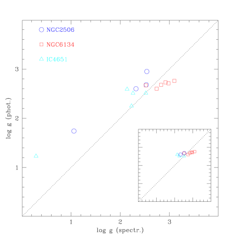
Figure 5: Spectroscopic gravities as a function of the derived photometric gravities. Different symbols are used for the 3 clusters. In the inset, only the clump stars and red giant stars are plotted, excluding the stars near the RGB-tip.

On the other hand, for stars at the RGB tip the agreement between the gravities computed with the two methods is much worse, with gravities derived from spectroscopy lower than those obtained from evolutionary masses.

In summary, when considering only clump stars, the agreement between spectroscopic gravities (i.e. obtained through the ionization equilibrium) and evolutionary gravities is on average good. This result leads to two relevant conclusions: (i) if our gravity values are correct, also our temperatures must be correct, hence our findings strongly support our temperature scale, which in turn translates in a reliable $metallicity$ scale; (ii) the small differences in gravity found with the two methods seem to hint convincingly against the existence of large departures from the LTE assumption (see Gratton et al. 1999): high quality spectra coupled with reliable oscillator strengths from laboratory experiments are able to provide solid Fe abundances for moderately warm stars.

As far as the cooler RGB tip stars are concerned, the situation is clearly more complex and less stable. In this case, we cannot exclude departures (even relevant) from LTE, since the lower atmospheric densities do favour non-local effects. Moreover, it is possible that the atmospheric structure of giant stars near the RGB tip is not well reproduced by presently existing model atmospheres of the Kurucz grid (see Dalle Ore 1993). For these reasons we believe it is safer to concentrate on warmer objects for this kind of analysis, in order to obtain more reliable results. In old OC’s the red clump stars are the best choice, given their temperatures and luminosities.

4 Reddening estimates from spectroscopy

Our effective temperatures are derived entirely from our spectra. As such, they are reddening-free and this approach allows us to give an estimate of the reddening toward the clusters which is independent of the photometric determinations. For this exercise, we used only the stars with T${}_{\rm eff}\leq$ 4400 K, i.e. on the clump or near it.

First we collected all the available broad and intermediate-band photometry for the analyzed stars. Johnson and Strömgren photometry was taken from the references indicated in Table 2, while JHK photometry was obtained from the 2MASS survey (from the Point Source Catalogue of the All-Sky Data Release, found at http://www.ipac.caltech.edu/2mass/) and transformed to the TCS system.

We then adopted the colour-temperature transformations by Alonso et al. (1996) and we entered our spectroscopic T_eff values in these relations to obtain de-reddened colours. Comparison with the observed colours provides an estimate of the $E(B-V)$ value.

Our final reddening values are derived as the weighted average of the reddening values as given from individual colours (adopting $E(b-y)=0.72E(B-V)$ and $E(V-K)=2.75E(B-V)$: Cardelli et al. 1989). As resulting errors, we adopted the larger between the internal error and the spread in the values obtained from individual colours.

Table 5: Values for the reddening as determined in the present paper; the three E(B-V) values for each cluster derived from individual colours, i.e. from (B-V), (b-y), and (V-K) respectively, are also given. The last line gives the adopted reddening.

	NGC 2506	NGC 6134	IC 4651
${\rm[Fe/H]}$	$-$0.20	+0.15	+0.11
Teff(ref.)	5000 K	5000 K	4500 K
E(B-V)BV	0.058$\pm$0.016	0.355$\pm$0.005	0.087$\pm$0.022
E(B-V)by		0.340$\pm$0.006	0.082$\pm$0.015
E(B-V)VK	0.076$\pm$0.007	0.388$\pm$0.005	0.080
E(B-V) adop.	0.073$\pm$0.009	0.363$\pm$0.014	0.083$\pm$0.011

Our results for the three clusters are listed in Table 5. The agreement with previous literature data is quite good (see Table 6). Overall, the differences are about 0.01 mag, with our values being slightly lower, on average by 0.008 mag. This implies that our temperatures might be a little too low: 0.01 mag in $B-V$ translates into an offset of about 20 K in the derived temperatures.

Table 6: Literature values for E(B-V) and E(b-y). SFD98=Schlegel et al. 1998; M+97=Marconi et al. 1997; K+01=Kim et al. 2001; D+02=Dias et al. 2002 (catalogue); KF91=Kjeldsen & Frandsen 1991; CM92=Clariá & Mermilliod 1992; B+99=Bruntt et al. 1999; AT+88=Anthony-Twarog et al. 1988; ATT00=Anthony-Twarog & Twarog 2000; M+02=Meibom et al. 2002

E(B-V)	E(b-y)	Reference & notes
NGC 2506
0.087		SFD98
0-0.07		M+97 ${\rm[Fe/H]}\simeq 0\leavevmode\nobreak\ {\rm to}\leavevmode\nobreak\ -0.4$
0.04$\pm$0.03		K+01
0.081		D+02 ${\rm[Fe/H]}$ = $-$0.37
NGC 6134
0.46$\pm$0.03		KF91
0.35$\pm$0.02		CM92 ${\rm[Fe/H]}$ = $-$0.05
0.365$\pm$0.006	0.263$\pm$0.004	B+99 ${\rm[Fe/H]}$ = +0.28
0.395		D+02 ${\rm[Fe/H]}$ = +0.18
IC 4651
0.086		AT+88
0.241		SFD98
0.086	0.062	ATT00 ${\rm[Fe/H]}$ = +0.08
0.099	0.071	ATT00 ${\rm[Fe/H]}$ = +0.12
	0.071	M+02 ${\rm[Fe/H]}\simeq+0.12$

Our temperatures for individual stars have attached random errors of about 40-50 K; since we use from 3 to 6 stars in each cluster, we expect errors of about 20-30 K per cluster, on average, hence 0.010-0.015 mag in the $E(B-V)$ value. Notice that the $\sim 90$ K estimated as the total internal error in temperature (see above, Sect. 3.2.1) do include not only a random component due to measurement errors, but also a systematic component due to the set of lines used (e.g. some lines always giving too high or too low abundances).

On the other hand, such a good agreement with literature data strengthens the reliability of our temperature scale, which is only 15 K (with 10-15 K of uncertainty) too low with respect to that by Alonso et al. (1996) from IRFM. This, in turn, might translate in our abundances being underestimated by (only) 0.01 dex.

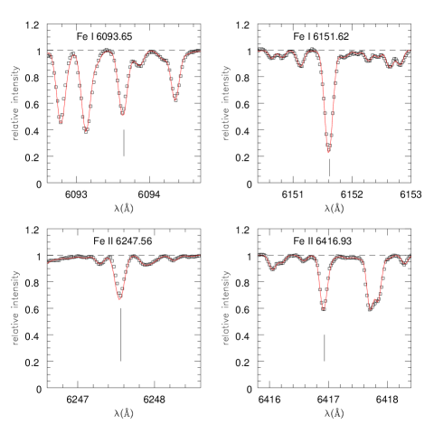
Figure 6: Comparison between the observed spectrum of the field metal-rich giant star HR 3627 (open squares) and the synthetic spectrum computed by optimizing the Kurucz line lists (solid lines). Small regions around 2 Fe I and 2 Fe II lines are shown.

5 Analysis with synthetic spectra: a check

When dealing with high-metallicity, rather cool stars, the line crowding might become rather difficult to treat simply with the standard method of line analysis. In order to check our results, we devised a new procedure based on an extensive comparison with spectrum synthesis:

• as a first step, line lists were prepared for selected regions of 2 Å centered on 44 Fe I lines and 9 Fe II lines chosen among those employed in our $EW$ analysis. These lines are in the wavelength range between 5500 and 7000 Å, and were selected because they have very precise $\log gf$’s, and are in comparatively less crowded spectral regions.

• For each region around Fe lines we computed a synthetic spectrum, starting from the Kurucz line list. Our list was then optimized by comparing it with the very high resolution ($R\sim 140,000$), high signal-to-noise spectrum of star HR 3627, a metal rich ([Fe/H]=+0.35) field giant. This star was selected because its spectrum is very line rich, due to the combination of low temperature and high metal abundance. Hence we expect that a line list compiled from this spectrum would be adequate to discuss even the most difficult cases among the stars in our sample. HR 3627 was observed with the SARG spectrograph mounted at the TNG, and its atmospheric parameters were derived from a full spectroscopic analysis and are: 4260/1.95/+0.35/1.20 (effective temperature, gravity, metal abundance and microturbulent velocity, respectively). An example of the optimized synthetic spectra for star HR 3627 is given in Figure 6, where two Fe I lines and two Fe II lines are showed, with the corresponding synthetic spectrum overimposed.

• After the line lists were optimized to well reproduce the spectrum of star HR 3627 (in particular for contaminants like CN, with large contribution in cool, metal-rich stars), we ran an automatic procedure that allows a line-by-line comparison of the observed spectrum and the synthetic spectra of the Fe lines.

• For each program star, 7 synthetic spectra were computed for each Fe line, varying the [Fe/H] ratios from $-$0.6 to +0.6 dex, in step of 0.2 dex.

• The $EW$’s of these synthetic spectra were measured by using a local pseudo-continuum that considers 2 small regions 0.8 Å wide on each side of the line. The measurements are then saved.

• The same lines are measured exactly in the same way on the observed spectra of the program stars.

• A line-to-line comparison is made between the observed $EW$’s and those measured on the synthetic spectra; the synthetic $EW$ that best matches the observed one is then adopted as the one giving the right abundance; examples of the matches obtained for star 421 in NGC 6134 are shown in Figure 7 .

• Finally, the resulting set of abundances are treated analogously to the traditional line analysis, temperatures and microturbulent velocities are derived by minimizing trends of abundances as a function of the excitation potential and line strengths and so on.

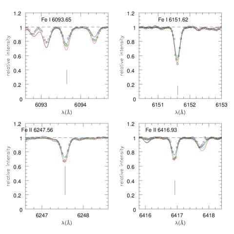
Figure 7: Comparison between the observed UVES spectrum of star 421 in NGC 6134 (open squares) with synthetic spectra of two Fe I and two Fe II lines (solid lines). The spectral synthesis was computed by using the atmospheric parameters appropriate to the star and 3 Fe abundances: [Fe/H]=-0.2, 0.0 and +0.2 dex from top to bottom, respectively.

As mentioned above, the first iteration using this technique showed a discrepancy with the values derived by line analysis for the NGC 2506 stars. For stars in NGC 6134 the disagreement was found for stars with FEROS, but not with UVES spectra, where the adopted fraction of high spectral points around the lines used for the local continuum tracing was higher ($1/2$ rather than $1/4$). This result leads us to conclude that the culprit was the location of the continuum, traced too high in the FEROS spectra of NGC 6134 and NGC 2506. We then repeated the $EW$ measurements by adopting $1/2$ as the fraction in the routine. This time, the improvement was significant and the agreement is fairly good, as shown in Table 7.

Table 7: Comparison between Fe I abundances from spectrum synthesis and $EW$ analysis for observed stars in NGC 2506, NGC 6134, and IC 4651.

Star	[Fe/H]I	$rms$	n	[Fe/H]I	Phase
	SS			$EW$
NGC 2506
459	$-$0.42	0.264	30	$-$0.37	RGBtip
438	$-$0.21	0.144	26	$-$0.18	clump
443	$-$0.15	0.079	19	$-$0.21	clump
456	$-$0.31	0.206	27	$-$0.21	RGB
NGC 6134
404	+0.12	0.145	22	+0.11	clump
929	+0.20	0.224	23	+0.24	clump
875	+0.10	0.253	29	+0.16	clump
428	+0.19	0.049	11	+0.22	clump
421	+0.09	0.148	16	+0.11	clump
527	+0.09	0.218	21	+0.05	clump
IC 4651
27	+0.16	0.200	25	+0.10	clump
76	+0.07	0.141	19	+0.10	clump
72	+0.18	0.172	21	+0.13	RGB
56	$-$0.68	0.238	24	$-$0.34	RGBtip
146	+0.18	0.198	23	+0.10	clump

The larger scatter in the Fe I abundances as obtained from spectrum synthesis is likely due to the method used to measure the local pseudo continuum around the Fe lines.

6 Results and discussion

Using the values derived for [Fe/H] only for the clump stars (Table 3) we have the following iron abundances: [Fe/H] = $-0.20$ ($\sigma$= 0.02, 2 stars) for NGC 2506, +0.15 ($\sigma$= 0.07, 6 stars) for NGC 6134, and +0.11 ($\sigma$= 0.01, 3 stars) for IC 4651.

Table 8: Literature values for metallicity, and methods used. The two values given for NGC 2506 by Marconi et al. correspond to the best reproductions of the observed CMDs with synthetic ones based on the Padova tracks (Bressan et al. 1993) at Z=0.008 and 0.02; note that further unpublished analyses with updated evolutionary tracks have shown that the solar solution should be excluded. The two solutions for IC 4651 given by Anthony-Twarog & Twarog correspond to two different calibrations of the intrinsic b-y colour versus metallicity.

Reference	${\rm[Fe/H]}$	E(B-V)	method
NGC 2506
this paper	$-$0.20	0.073	high-res sp.
Geisler et al. 1992	$-$0.58		Washington ph.
Friel & Janes 1993	$-$0.52	0.05	low-res sp.
Marconi et al. 1997	$\sim-$0.4 to 0.0	0.05 to 0	synthetic CMD
Twarog et al. 1997	$-$0.38	0.05	low-res sp.+ DDO
Friel et al. 2002	$-$0.44	0.05	low-res sp.
NGC 6134
this paper	+0.15	0.363	high-res sp.
Clariá & Mermilliod 1992	$-$0.05	0.35	Wash. + DDO
Twarog et al. 1997	+0.18	0.35 -0.39	DDO
Bruntt et al. 1999	+0.28	0.365	Strömgren
IC 4651
this paper	+0.11	0.083	high-res sp.
Twarog et al. 1997	+0.09	0.11 - 0.12	DDO
Anthony-Twarog & Twarog 2000	+0.077	0.086	Strömgren
	+0.115	0.099	Strömgren
Meibom et al. 2002	$\sim$ +0.12	0.10	CMD (Yale)

6.1 Comparison with other determinations

None of these clusters has a previous metallicity measure based on high resolution spectroscopy, but they have been the subject of many studies; we present in Table 8 literature metal abundance, based on low resolution spectroscopy, or photometric metallicity indicators (in DDO, Washington and Strömgren filters), or comparison of observed CMDs with theoretical isochrones/tracks. The reader is referred to the original papers for detailed explanations, and we give here only a few notes on some of the works.

Twarog et al. (1997) tried to derive in a homogeneous way the properties of a large sample of OC’s, and re-examined literature data to find distances, reddenings and metallicities; for these they selected two methods, DDO photometry and the low resolution spectroscopy of Friel & Janes (1993), putting the two systems on the same scale. Values cited in Table 8 come from their Tables 1 and 2.

Friel & Janes (1993) collected low resolution spectra of giants of a quite large sample of OC’s; for an update, see Friel et al. (2002).

Marconi et al. (1997) used the synthetic CMD technique to determine at the same time distance, reddening, age, and approximate metallicity of NGC 2506; they employed three different sets of evolutionary tracks (Padova, Geneva, and FRANEC) finding that, for Z = 0.008 and 0.01 ([Fe/H] $\simeq-0.4$ and $-$0.3), they were able to reproduce the observed CMD, although the metal-poor solutions were preferred. A similar method was employed by Meibom et al. (2002) for IC 4651, but they only considered the Yale isochrones.

Finally, Anthony-Twarog & Twarog (2000) give two alternative solutions for IC 4651, based on different relations for the intrinsic Strömgren colours.

When we compare our findings with literature values, we find i) that our abundance for NGC 2506 is generally much higher, ii) that NGC 6134 has strongly discrepant determinations, and iii) that IC 4651 is in much better agreement with past works. We emphasize, though, that fine abundance analysis of high resolution, high signal to noise spectra is the most precise method to measure the elemental composition. Given also the tests done on our temperature and gravity scale, we feel confident about the derived metallicities.

Finally, note that, adopting our metallicity ([Fe/H] = +0.15), and the age derived by Bruntt et al. (1999: 0.69 $\pm$ 0.10 Gyr), NGC 6134 appears almost a twin of the Hyades for which Perryman et al. (1998) give [Fe/H]=+0.14 $\pm$ 0.05, age 0.625 $\pm$ 0.05 Gyr, and distance modulus (m-M)₀ = 3.33 $\pm$ 0.01. The similarity (although the clump stars in NGC 6134 are more numerous) is confirmed by the absolute magnitude of the clump stars, which span a similar range (M_V $\sim$ 0.2 - 0.5) in the two OC’s.

7 Summary

We derived precise metallicities for 3 open clusters (NGC 2506, NGC 6135 and IC 4651) from high resolution spectroscopy, using both the traditional line analysis and extensive comparison with synthetic spectra. Our adopted temperature scale from excitation equilibrium gives consistent values of reddenings in very good agreement with previous, independent estimates of $E(B-V)$ for the three clusters. This finding strongly supports the adopted temperature scale and, in turn, the derived metallicity scale. The nice agreement between spectroscopic and evolutionary gravities also indicates the goodness of the adopted temperatures and leaves little space for the effect of possible departures from the LTE assumption. Our approach is then well suited to derive metal abundances of stellar populations with a [Fe/H] ratio around solar.

- (1) Allende Prieto, C., Barklem, P.S., Lambert, D.L., V Cunha, C. 2004, A&A, in press (astro-ph/0403108)
- (2) Alonso, A., Arribas, S. & Martinez-Roger, C. 1996, A&A, 313, 873
- (3) Alonso, A., Arribas, S. & Martinez-Roger, C. 1999, A&AS, 140, 261
- (4) Anthony-Twarog, B.J., Mukherjee, K., Twarog. B.A., & Caldwell, N. 1988, AJ, 95, 1453
- (5) Anthony-Twarog, B.J., & Twarog, B.A. 2000, 119, 2282
- (6) Bragaglia, A., et al. 2001, AJ, 121, 327
- (7) Bragaglia, A., Tosi, M., Marconi, G., & Carretta, E.: 2000, in ’The Evolution of the Milky Way. Stars vs Clusters’, F.Giovannelli & F.Matteucci eds (Kluwer, Dordrecht), 255, 281
- (8) Bragaglia, A., Tosi, M., Carretta, E., & Marconi, G. 2004, in Stellar Populations 2003, http://www.mpa-garching.mpg.de/stelpops/
- (9) Bressan, A., Fagotto, F., Bertelli, G., & Chiosi, C. 1993, A&AS, 100, 647
- (10) Bruntt, H., Frandsen, S., Kjeldsen, H., & Andersen, M.I. 1999, A&AS, 140, 135
- (11) Cardelli, J.A., Clayton, G.C., & Mathis, J.S. 1989, ApJ, 345, 245
- (12) Carraro, G., Ng, Y.K., & Portinari, L. 1998, MNRAS, 296, 1045
- (13) Carretta, E., Gratton, R.G., Cohen, J.G., Beers, T.C., & Christlieb, N. 2002, AJ, 124, 481
- (14) Cayrel, R. 1989 in The Impact of Very High S/N Spectroscopy on Stellar Physics, eds. G. Cayrel de Strobel and M. Spite (Dordrecht:Kluwer), 345
- (15) Chiu, L.-T. & Van Altena, W.F. 1981, ApJ, 243, 827
- (16) Cutri, R.M., et al. 2003, VizieR On-line Data Catalog: II/246, Originally published in: University of Massachusetts and Infrared Processing and Analysis Center, (IPAC/California Institute of Technology)
- (17) Clariá, J.J., & Mermilliod, J.-C. 1992, A&AS, 95, 429
- (18) Dalle Ore, C. 1993, Ph.D. thesis
- (19) Dias, W.S., Alessi, B.S., Moitinho, A.,& Lépine, J.R.D. 2002, A&A, 389, 871
- (20) Eggen, O.J. 1971, ApJ, 266, 87
- (21) Friel, E.D. 1995, ARA&A, 33, 381
- (22) Friel, E.D.& Janes K.A 1993, A&A, 267, 75
- (23) Friel, E.D., et al. 2002, AJ, 124, 2693
- (24) Geisler, D., Clariá, J.J., & Minniti, D. 1992, AJ, 104, 1992
- (25) Girardi, L., Bressan, A., Bertelli, G., & Chiosi, C. 2000, A&AS, 141, 371
- (26) Gratton, R.G., Carretta, E., Eriksson, K., & Gustafsson, B. 1999, A&A, 350, 955
- (27) Gratton, R.G., Carretta, E., Claudi, R.., Lucatello, S., & Barbieri, M. 2003, A&A, 404, 187
- (28) Jennens, P.A., & Helfer, H.L. 1975, MNRAS, 172, 681
- (29) Kalirai, J.S. & Tosi, M. 2004, MNRAS, in press
- (30) Kim S.L., et al. 2001, AcA, 51, 49
- (31) Kjeldsen, H., & Frandsen, S. 1991, A&AS, 87, 119
- (32) Kurucz, R.L. 1995, CD-ROM 13, Smithsonian Astrophysical Observatory, Cambridge
- (33) Lindoff, U. 1972, A&AS, 7, 231
- (34) Maciel, W.J., & Chiappini, C., 1994, Astrophys.& Sp.Sc., 219, 231
- (35) Maciel, W.J., Costa, R.D.D., & Uchida, M.M.M. 2003, A&A, 397, 667
- (36) Maciel, W.J., & Köppen, J., 1993, A&A, 282, 436
- (37) Marconi, G., Hamilton, D., Tosi, M., & Bragaglia, A. 1997, MNRAS, 291, 763
- (38) Meibom, S. 2000, A&A, 361, 929
- (39) Meibom S., Andersen J., & Nordstrom B. 2002, A&A, 386, 187
- (40) Mermilliod, J.-C. 1995, in Information and On-Line Data in Astronomy, D. Egret, M.A. Albrecht eds, Kluwer Academic Press (Dordrecht), p. 127
- (41) Mermilliod, J.-C., Andersen, J., Nordstroem, B., & Mayor M. 1995, A&AS, 229, 53
- (42) Minniti, D. 1995, A&AS, 113, 299
- (43) Pasquali, A., & Perinotto, M., 1993, A&A, 280, 581
- (44) Perryman, M.A.C., et al. 1998, A&A, 331, 81
- (45) Schlegel, D.J., Finkbeiner, D.P., & Davis, M. 1998, ApJ, 500, 525
- (46) Tosi, M.: 1996, ’Comparison of chemical evolution models for the galactic disk’ in ’From stars to galaxies’, C.Leitherer, U.Fritze-von Alvensleben, J.Huchra eds, ASP Conf.Ser., 98, 299
- (47) Tosi, M. 2000, ’The chemical evolution of the Galaxy’, in ’The Evolution of the Milky Way. Stars vs Clusters’, F.Giovannelli & F.Matteucci eds (Kluwer, Dordrecht ), 505
- (48) Tosi, M., Greggio, L., Marconi, G., & Focardi, P. 1991, AJ, 102, 951
- (49) Twarog, B.A., Ashman, K.M., & Anthony-Twarog, B.J. 1997, AJ 114, 2556