High mass X-ray binaries in the LMC: dependence on the stellar population age and the “propeller” effect

We study the population of compact X-ray sources in the Large Magellanic Cloud using the archival data of the XMM-Newton observatory. The total area of the survey is $\approx 3.8$ square degrees with a limiting sensitivity of $\approx 10^{-14}$ erg/s/cm², corresponding to a luminosity of $\approx 3\cdot 10^{33}$ erg/s at the LMC distance. Out of $\sim 460$ point sources detected in the 2–8 keV energy band, the vast majority are background CXB sources, observed through the LMC. Based on the properties of the optical and near-infrared counterparts of the detected sources we identified 9 likely HMXB candidates and 19 sources, whose nature is uncertain, thus providing lower and upper limits on the luminosity distribution of HMXBs in the observed part of LMC. When considered globally, the bright end of this distribution is consistent within statistical and systematic uncertainties with extrapolation of the universal luminosity function of HMXBs. However, there seems to be fewer low luminosity sources, $\log(L_{X})\la 35.5$, than predicted. We consider the impact of the “propeller effect” on the HMXB luminosity distribution and show that it can qualitatively explain the observed deficit of low luminosity sources.

We found significant field-to-field variations in the number of HMXBs across the LMC, which appear to be uncorrelated with the star formation rates inferred by the FIR and $H_{\alpha}$ emission. We suggest that these variations are caused by the dependence of the HMXB number on the age of the underlying stellar population. Using the existence of large coeval stellar aggregates in the LMC, we constrain the number of HMXBs as a function of time $\tau$ elapsed since the star formation event in the range of $\tau$ from $\sim 1-2$ Myr to $\sim 10-12$ Myr.

1 Introduction.

First imaging X-ray observations of the Large Magellanic Cloud with Einstein (Wang et al., 1991) and ROSAT (Haberl & Pietsch, 1999) observatories revealed a moderate population of several tens of X-ray sources associated with this closest neighbor of the Milky Way. While in the soft X-ray band a large fraction of these sources are supernovae remnants, at higher energies, above $\sim$ few keV, X-ray binaries provide the dominant contribution. For example, based on the spectral hardness of bright ROSAT sources, Kahabka (2002) identified in the entire LMC $\sim 20-30$ probable X-ray binary candidates with luminosity exceeding $L_{X}\ga{\rm few}\times 10^{35}$ erg/s.

The relative numbers of high and low mass X-ray binaries (H or LMXBs) are defined by the specific star formation rate SFR/$M_{*}$ of the host galaxy (Grimm et al., 2003; Gilfanov, 2004). Owing to rather low mass, $M_{*}\sim 2\cdot 10^{9}$ M_☉ (section 3.2), and moderate star formation rate (SFR) of $\sim 0.5\leavevmode\nobreak\ M_{\sun}$ yr^-1 (section 3.3), this quantity is rather high for the LMC, with a SFR/$M_{*}\sim(2-3)\cdot 10^{-10}{\rm\leavevmode\nobreak\ yr}^{-1}$, exceeding by a factor of $\sim 5-10$ that of our Galaxy. Correspondingly, the ratio of the expected numbers of bright, $\log(L_{X})\ga 35$, X-ray binaries in the LMC equals $N_{LMXB}:N_{HMXB}\sim 1:7$ (Gilfanov, 2004), i.e. is nearly opposite to that observed in the Milky Way (Grimm et al., 2002). The absolute number of HMXBs in the LMC is expected to be $\sim 1/4$ of the number observed in our Galaxy, corresponding to the ratio of star formation rates in these two galaxies.

As has been shown by Grimm et al. (2003), the X-ray luminosity function (XLF) of HMXBs obeys, to the first approximation, a universal power law distribution with a differential slope of $\approx 1.6$, whose normalization is proportional to the star formation rate of the host galaxy. The validity of this universal HMXB XLF has been established in a broad range of the star formation rates and regimes and in the luminosity range $\log(L_{X})\ga 35.5-36$. Based on the ASCA observations of the Small Magellanic Cloud and on the behavior of the integrated X-ray luminosity of distant galaxies located at redshifts $z\sim 0.3-1.3$ observed by Chandra in the Hubble Deep Field North, Grimm et al. (2003) tentatively suggested that the HMXB XLF is not dramatically affected by metallicity variations.

Study of the population of high mass X-ray binaries in the LMC is of importance for several reasons:

1. The Magellanic Clouds are known to have a significant under-abundance of metals (Westerlund, 1997). For the interstellar medium and young stellar population in the LMC the metal abundance is approximately $\sim 1/3$ of the solar value (Westerlund, 1997; Garnett, 1999; Korn et al., 2002). The effects of the metallicity variations on the population of X-ray binaries are poorly understood. Study of the LMC, a galaxy with a relatively well-known chemical composition gives a unique opportunity to investigate such effects observationally.

2. Owing to the proximity of the LMC, the weakest sources become reachable with a moderate observing time. Indeed, the sensitivity of a typical Chandra or XMM-Newton observation, $\sim 10^{-14}$ erg/s/cm², corresponds to the luminosity of $\sim 3\cdot 10^{33}$ erg/s at the LMC distance. This opens the possibility to study the low luminosity end of the HMXB XLF, extending by $\sim 2-3$ orders of magnitude towards low luminosities the luminosity range studied by Grimm et al. (2003). Among other applications, this will allow study of the impact of propeller effect (Illarionov & Sunyaev, 1975) on the luminosity distribution of HMXBs.

3. The proximity and moderate inclination angle of the Magellanic Clouds (especially that of the LMC) allows one to construct Herzsprung-Russel diagrams and accurately determine ages, star formation history and initial mass function of various components of the stellar population. In particular, large aggregates of young and coeval stellar populations of ages ranging from $\la 1-2$ Myr to $\ga 50-100$ Myr were discovered in the LMC. The most extreme examples of these are the LMC 4 supergiant shell (Braun et al., 1997) and R136 (HD 38268) stellar cluster near the center of the nebula 30 Dor (Massey & Hunter, 1998). Combined with HMXB number counts in the optically studied regions, these results provide a unique possibility to directly determine the efficiency of HMXB formation as a function of time elapsed since the star formation event.

The proximity of the LMC, on the other hand, creates several difficulties in its studies. Due to its large angular extent on the sky, $\sim 10\degr\times 10\degr$, multiple mosaiced observations are required to achieve a meaningful coverage of the galaxy. The low surface density of X-ray binaries results in a large fraction of foreground stars and background AGNs among the detected sources, thus creating the problem of separating true galactic members from interlopers. This was one of the main obstacles in the earlier studies of X-ray binaries in the LMC with moderate angular resolution, insufficient for reliable identification of X-ray sources with optical catalogs. With the advent of Chandra and XMM-Newton observatories, the latter problem is to a large extent alleviated.

Table 1: List of XMM-Newton observations used for analysis

Obs. ID	Target	R.A.	Dec.	Instrument	Exposure	SFR(1)
		J2000	J2000		ksec	$M_{\sun}$/yr
0113000501	0519-69.0	05 19 23	-69 00 52	MOS1+MOS2	25+47	$4.13\cdot 10^{-3}$
0111130201	2E 0509.5–6734	05 09 16	-67 31 41	MOS1+MOS2	34+34	$7.77\cdot 10^{-4}$
0062340101	2E 0453.8–6834	04 53 41	-68 31 07	MOS1+MOS2	16+16	$1.49\cdot 10^{-3}$
0111130301	2E 0525.3–6601	05 25 13	-65 59 38	MOS1+MOS2	9.5+9.5	$1.83\cdot 10^{-3}$
0134520701	AB Dor	05 28 35	-65 28 30	MOS1+MOS2	48+48	$2.92\cdot 10^{-4}$
0123510101	CAL 83	05 43 33	-68 24 07	MOS1+MOS2	10+10	$1.37\cdot 10^{-3}$
0104060101	LMC Deep field	05 31 17	-65 55 58	MOS1+MOS2	38+38	$6.35\cdot 10^{-4}$
0109990201	DEM L71	05 05 49	-67 54 11	MOS1+MOS2	22+23	$1.30\cdot 10^{-3}$
0109990101	LHA 120–N63A	05 35 51	-66 00 32	MOS1+MOS2	9.6+9.6	$1.38\cdot 10^{-3}$
0094410101	LMC-2(f1)	05 42 35	-69 03 20	PN	8.8	$9.74\cdot 10^{-3}$
0094410201	LMC-2(f2)	05 42 58	-69 28 22	PN	8.8	$5.51\cdot 10^{-3}$
0094410401	LMC-2(f4)	05 46 48	-69 33 39	MOS1+MOS2	5.2+5.2	$4.60\cdot 10^{-3}$
0126500101	LMC X-3	05 38 44	-64 06 11	MOS1+MOS2	20+20	$7.82\cdot 10^{-5}$
0113000301	N103B	05 08 41	-68 43 53	MOS2	23ks	$4.52\cdot 10^{-3}$
0089210701	N120	05 18 37	-69 37 56	MOS1+MOS2	36+36	$5.76\cdot 10^{-3}$
0089210901	N206	05 31 51	-70 58 39	MOS1+MOS2	24+24	$3.35\cdot 10^{-3}$
0071940101	N51D	05 26 05	-67 27 21	MOS1+MOS2	32+32	$3.37\cdot 10^{-3}$
0127720201	Nova LMC 2000	05 24 41	-70 14 00	MOS1+MOS2	22+22	$1.34\cdot 10^{-3}$
0113000401	PSR 0540–69.3	05 40 02	-69 21 19	MOS2	35	$2.29\cdot 10^{-2}$
0113020201	PSR J0537–6909	05 37 57	-69 08 52	MOS1	37	$5.08\cdot 10^{-2}$
0008020101	RXJ0439.8–6809	04 39 57	-68 07 27	MOS1+MOS2	15+15	$1.83\cdot 10^{-4}$
0089210601	SNR0450-709	04 50 26	-70 48 48	MOS1+MOS2	56+57	$6.19\cdot 10^{-4}$
0137160201	YYMen	04 58 12	-75 15 01	MOS1+MOS2	87+87	$3.50\cdot 10^{-4}$

1 – star formation rate within the XMM-Newton FOV determined form the FIR flux as described in sections 3.3 and 3.4.

In the present paper we study the population of X-ray binaries in the LMC based on archival XMM-Newton data. The distance modulus of the LMC is $m-M=18.45\pm 0.10$ (Westerlund, 1997), corresponding to the distance of $D\approx 50$ kpc. The interstellar reddening varies across the LMC, with typical values in the range $E_{B-V}\approx 0.05-0.2$ (Westerlund, 1997). A value of $E_{B-V}=0.075$ corresponding to the direction towards the nominal center of the LMC is used throughout the paper.

The paper is structured as follows. XMM-Newton observations and data analysis are described in section  2. In section  3 we discuss the nature of detected X-ray sources. In section  4 we describe the HMXB search procedure and its results. Resulting HMXB luminosity function and the CXB log(N)–log(S) are presented in section  5. The impact of the propeller effect on the HMXB luminosity function is considered in section  6. In section  7 we discuss observed spatial non-uniformity of the $N_{HMXB}/SFR$ ratio and its dependence on the age of the underlying stellar population. Our results are summarized in section 8.

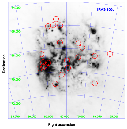
Figure 1: Far-infrared (IRAS, $100\mu$) map of the $10\degr\times 10\degr$ region around the Large Magellanic Cloud. Circles show fields of view of the XMM–Newton observations used for the analysis.

2 Observations and data analysis.

We have selected 23 XMM-Newton archival observations with the pointing direction towards the LMC and with a sensitivity better than $\sim{\rm few}\times 10^{-14}$ erg/s/cm² in the 2–10 keV energy band. These observations are listed in Table 1. Fig.1 shows their fields of view, overlayed on the far-infrared map (IRAS, $100\mu$) of the Large Magellanic Cloud.

The observations were processed with the standard SAS task chain. After filtering out high background intervals we extracted images in the 2–8 keV energy band. This energy range was chosen to minimize the fraction of supernovae remnants, cataclysmic variables and foreground stars among detected sources, generally having softer spectra than high mass X-ray binaries. To improve the sensitivity of the survey, images from MOS1 and MOS2 detectors were merged. If both MOS and PN data were available, we used the data having higher sensitivity and smaller number of spurious sources.

2.1 Source detection.

The source detection on the extracted images was performed with standard SAS tasks eboxdetect and emldetect. The value of the threshold likelihood $L$ used in the emldetect task to accept or reject detected source was chosen as follows. We simulated a number of images with Poisson background counts (without sources). Each of the generated images was analyzed with the full sequence of source detection procedures using different values of the emldetect threshold likelihood $L$ and for each trial value of $L$ the number of detected “sources” was counted. The final value of the threshold likelihood, $L=22$, was chosen such that the total number of spurious detections was $\la 3$ per 23 images. Note that due to the definition of the threshold likelihood in the emldetect task, this value should not be interpreted as $L=-\ln(p)$, with $p$ equal to the probability of detecting a given number of counts due to the statistical fluctuation of the Poisson noise.

The obtained images were visually inspected and the source lists were manually filtered of spurious sources near bright sources and arcs caused by a single reflection. All extended sources were removed from the lists. The 2–8 keV source counts were converted to the 2–10 keV energy flux assuming a power law spectrum with photon index 1.7 and N_H=6$\cdot 10^{20}$cm^-2. The energy conversion factors are ecf_MOS=2.27$\cdot 10^{-11}$ erg/cm² and ecf_PN=8.0$\cdot 10^{-12}$ erg/cm². The final merged source list contains $\approx 460$ sources. Their flux distribution is plotted in Fig.3. The sources with flux $\geq 10^{-13}$ erg/s/cm² are listed in Table 2.

2.2 Boresight correction

For several XMM observations we performed boresight correction using the SAS task eposcorr and optical sources from the USNO-B catalogue (Monet et al., 2003). The correction was applied if any of the following conditions was satisfied:

1. Optical counterparts for 2 or more well-known sufficiently bright X-ray sources were found.

2. Only one well-known X-ray source with an optical counterpart in USNO is present. Offsets calculated by the eposcorr task statistically significantly reduce its displacement from the optical counterpart.

3. The offsets calculated by the eposcorr task using optical data in different non-overlapping magnitude ranges were consistent with each other.

2.3 Correction for incompleteness

To compute the flux-dependent survey area, we reproduced the likelihood calculation procedure used in the emldetect task and computed the point source detection sensitivity map for each observation. The sensitivity in a given pixel of the image was defined as the count rate of the source located in this pixel, whose likelihood of detection was equal to the threshold value used in the emldetect task. Combining sensitivity maps of all observations we calculated the survey area as a function of flux (Fig. 2). From Fig. 2 one can see that the incompleteness effects become important at fluxes $\la 10^{-13}$erg/s/cm². In the high flux limit, the total area of the survey equals $A_{\rm tot}\approx 3.77$ deg².

The inverse area of the survey can be used to correct the observed differential log(N)–log(S) distribution:

$$\left(\frac{dN}{dS}\right)_{corrected}=\frac{1}{A(S)}\cdot\left(\frac{dN}{dS}\right)_{observed}$$ (1)

where A(S) is the survey area at flux S. The corrected cumulative log(N)–log(S) distribution can be obtained as follows:

$$N(>S)=\sum_{S_{j}>S}{\frac{1}{A(S_{j})}},$$ (2)

where $S_{j}$ is the flux of the j-th source. With these corrections, the flux distributions are normalized per deg². The flux distribution, corrected for incompleteness effects, is plotted as the thick histogram in Fig.3.

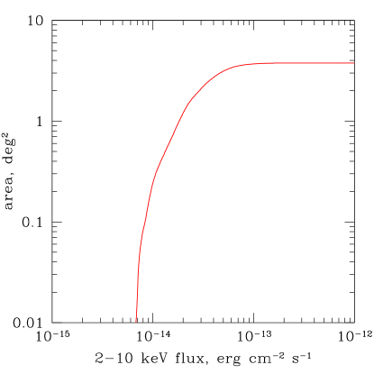
Figure 2: The survey area as a function of 2–10 keV flux, calculated as described in section 2.3.

Table 2: List of detected sources with 2–10 keV flux $F_{X}\geq 10^{-13}$ erg/s/cm²

Source ID	$F_{X}$[2–10 keV]	$L_{X}$[2–10 keV]1	Rmag2	Fx/Fopt	Comments
	erg/s/cm2	erg/s
XMMUJ053856.7–640503	$2.67\cdot 10^{-11}$	$8.0\cdot 10^{36}$	16.7	33	HMXB LMC X-3
XMMUJ054011.5–691953	$2.45\cdot 10^{-11}$	$7.4\cdot 10^{36}$			Crab-like pulsar PSR B0540–69
XMMUJ052844.9–652656	$1.30\cdot 10^{-11}$		6.4∗	0.0012	foreground star ABDor
XMMUJ045818.0–751637	$6.06\cdot 10^{-12}$		7.5∗	0.0016	foreground star YYMen
XMMUJ053747.4–691020	$5.39\cdot 10^{-12}$	$1.6\cdot 10^{36}$			Crab-like pulsar PSRJ0537–6910
XMMUJ053113.1–660707	$3.01\cdot 10^{-12}$	$9.0\cdot 10^{35}$	14.0	0.31	HMXB Be EXO053109–6609
XMMUJ052402.1–701108	$2.08\cdot 10^{-12}$				AGN RXJ0524.0-7011
XMMUJ043831.4–681203	$8.88\cdot 10^{-13}$	$2.7\cdot 10^{35}$
XMMUJ053844.2–690608	$8.35\cdot 10^{-13}$	$2.5\cdot 10^{35}$			W–R stars (?) in R136
XMMUJ053011.3–655123	$6.59\cdot 10^{-13}$	$2.0\cdot 10^{35}$	14.7	0.13	HMXB Be (?) 272s pulsar3
XMMUJ050550.2–675018	$5.80\cdot 10^{-13}$	$1.7\cdot 10^{35}$	17.6	1.5
XMMUJ053115.4–705350	$5.25\cdot 10^{-13}$	$1.6\cdot 10^{35}$	13.8	0.043
XMMUJ053218.6–710746	$4.28\cdot 10^{-13}$	$1.3\cdot 10^{35}$	17.9	1.6
XMMUJ053833.9–691157	$3.65\cdot 10^{-13}$	$1.1\cdot 10^{35}$	17.8	1.3
XMMUJ050026.6–750449	$3.50\cdot 10^{-13}$	$1.1\cdot 10^{35}$	18.2	1.7
XMMUJ052847.3–653956	$2.70\cdot 10^{-13}$	$8.1\cdot 10^{34}$
XMMUJ045208.7–705652	$2.33\cdot 10^{-13}$	$7.0\cdot 10^{34}$
XMMUJ045637.9–751015	$2.06\cdot 10^{-13}$	$6.2\cdot 10^{34}$	18.3	1.1
XMMUJ054134.7–682550	$2.04\cdot 10^{-13}$	$6.1\cdot 10^{34}$	14.0	$0.020$
XMMUJ052312.9–701531	$1.94\cdot 10^{-13}$	$5.8\cdot 10^{34}$
XMMUJ050526.6–674313	$1.91\cdot 10^{-13}$		10.84	0.0011	foreground star GSC 9161.1103
XMMUJ053528.5–691614	$1.89\cdot 10^{-13}$	$5.7\cdot 10^{34}$			SNR SN1987A
XMMUJ054151.2–682609	$1.75\cdot 10^{-13}$	$5.3\cdot 10^{34}$
XMMUJ045244.2–704821	$1.71\cdot 10^{-13}$	$5.1\cdot 10^{34}$
XMMUJ050833.2–685427	$1.70\cdot 10^{-13}$	$5.1\cdot 10^{34}$
XMMUJ052403.1–673606	$1.67\cdot 10^{-13}$	$5.0\cdot 10^{34}$	18.3	0.91
XMMUJ053041.1–660535	$1.66\cdot 10^{-13}$	$5.0\cdot 10^{34}$	18.2	0.83
XMMUJ053810.0–685658	$1.58\cdot 10^{-13}$	$4.7\cdot 10^{34}$
XMMUJ052947.7–655643	$1.51\cdot 10^{-13}$	$4.5\cdot 10^{34}$	14.8	0.033	HMXB Be/X transient RXJ0529.8–6556
XMMUJ045219.8–684151	$1.49\cdot 10^{-13}$	$4.5\cdot 10^{34}$
XMMUJ053734.9–641012	$1.46\cdot 10^{-13}$	$4.4\cdot 10^{34}$
XMMUJ053909.8–640310	$1.33\cdot 10^{-13}$	$4.0\cdot 10^{34}$
XMMUJ051832.5–693521	$1.32\cdot 10^{-13}$	$4.0\cdot 10^{34}$
XMMUJ051747.0–685458	$1.32\cdot 10^{-13}$	$4.0\cdot 10^{34}$
XMMUJ051003.9–671858	$1.31\cdot 10^{-13}$	$3.9\cdot 10^{34}$
XMMUJ054237.8–683205	$1.29\cdot 10^{-13}$	$3.9\cdot 10^{34}$
XMMUJ050736.6–684752	$1.23\cdot 10^{-13}$	$3.7\cdot 10^{34}$
XMMUJ053257.7–705113	$1.23\cdot 10^{-13}$	$3.7\cdot 10^{34}$	19.0∗	1.3
XMMUJ052422.4–672020	$1.22\cdot 10^{-13}$	$3.7\cdot 10^{34}$
XMMUJ052353.7–672824	$1.21\cdot 10^{-13}$	$3.6\cdot 10^{34}$
XMMUJ054212.6–692442	$1.19\cdot 10^{-13}$	$3.6\cdot 10^{34}$	19.3∗	1.6
XMMUJ054543.2–682528	$1.17\cdot 10^{-13}$	$3.5\cdot 10^{34}$
XMMUJ050048.6–750653	$1.15\cdot 10^{-13}$	$3.5\cdot 10^{34}$
XMMUJ053632.6–655644	$1.14\cdot 10^{-13}$	$3.4\cdot 10^{34}$
XMMUJ045137.0–710210	$1.14\cdot 10^{-13}$	$3.4\cdot 10^{34}$
XMMUJ053841.7–690514	$1.03\cdot 10^{-13}$	$3.1\cdot 10^{34}$			W–R stars (?) in R140
XMMUJ052558.0–701107	$1.03\cdot 10^{-13}$		11.0	0.00068	foreground star, K2IV-Vp, RS CVn
XMMUJ052952.9–705850	$1.02\cdot 10^{-13}$	$3.1\cdot 10^{34}$

1 – calculated assuming distance to LMC 50 kpc.
2 – apparent magnitude in the R-band of the optical counterpart from GSC2.2.1 catalogue (Morrison & McLean, 2001), located within 3.6 arcsec from the X-ray source.
3 – Haberl et al. (2003)
4 – apparent R-band magnitude from the USNO-B catalogue (Monet et al., 2003).

3 Nature of X-ray sources in the field of LMC

3.1 Background and foreground sources

The total number of sources with the flux $F_{X}[2-10{\rm\leavevmode\nobreak\ kev}]>3.34\cdot 10^{-14}$ erg/s/cm² is 181. After correction for the survey incompleteness (eq.2) this number becomes $N_{\rm obs}(>3.3\cdot 10^{-14})\approx 214$. According to the CXB $\log(N)-\log(S)$ determined by Moretti et al. (2003), the total number of CXB sources expected in the field of 3.77 deg² is $N_{CXB}\approx 218_{-58}^{+117}$. The errors in this estimate were computed from the uncertainty of the normalization of the CXB $\log(N)-\log(S)$ relation, as given by Moretti et al. (2003). From the comparison of these numbers it is obvious that the majority of the detected sources are background AGNs.

A significantly less important source of contamination are X-ray sources associated with foreground stars in the Galaxy (no known Galactic X-ray binaries were located in the field of view of XMM observations). There were seven well-known bright nearby stars with 2–10 keV flux exceeding $10^{-14}$ erg/s/cm². All these were excluded from the final source list.

3.2 Low mass X-ray binaries

Given the limiting sensitivity of the survey, $F_{X}\sim(1-3)\cdot 10^{-14}$ erg/s/cm², corresponding to the luminosity $L_{X}\sim 3\cdot 10^{33}-10^{34}$ erg/s at the LMC distance, the intrinsic LMC sources are dominated by X-ray binaries. Their total number is proportional to the stellar mass (LMXB) and star formation rate (HMXB) of the galaxy.

The total stellar mass of the LMC can be estimated from the integrated optical luminosity. According to the RC3 catalog (de Vaucouleurs et al., 1991), the reddening-corrected V-band magnitude of the LMC equals $V_{To}\approx 0.13$, corresponding to the total V-band luminosity of $L_{V}\approx 1.9\cdot 10^{9}$ $L_{\sun}$. From the dereddened optical color $(B-V)_{To}\approx 0.44$ (de Vaucouleurs et al., 1991) and using results of Bell & de Jong (2001), the V-band mass-to-light ratio is $(M/L)_{V}\approx 0.77$ in solar units, giving the total stellar mass of the LMC $M_{*}\approx 1.5\cdot 10^{9}\leavevmode\nobreak\ M_{\sun}$. Using more recent determination of the $(B-V)_{To}\approx 0.54$ (Bothun & Thompson, 1988), the V-band mass-to-light ratio is $(M/L)_{V}\approx 1.0$, increasing the total stellar mass estimate to $M_{*}\approx 2.0\cdot 10^{9}\leavevmode\nobreak\ M_{\sun}$. For the stellar mass of $\approx(1.5-2.0)\cdot 10^{9}$ M_☉, using results of Gilfanov (2004), $\sim 8-10$ LMXBs with luminosity $L_{X}\ga 10^{35}$ erg/s are expected in the entire galaxy.

3.3 Star formation rate in the LMC

Below we compare the estimates of the star formation rate in the LMC, obtained from different SFR indicators. As is commonly used, the SFR values quoted below refer to the formation rate of stars in the $0.1-100$ M_⊙ range, assuming Salpeter’s initial mass function (IMF).

Based on the total $H_{\alpha}$ luminosity of the LMC and applying an extinction correction of $A(H_{\alpha})\approx 0.3$ Kennicutt et al. (1995) estimated the star formation rate of

$${\rm SFR}(H_{\alpha})=0.26\leavevmode\nobreak\ M_{\odot}/{\rm yr}$$ (3)

As was discussed by Kennicutt (1991), $H_{\alpha}$-based SFR indicators can underestimate the total star formation rate in the Magellanic Clouds, due to uncertainty of the escaping fraction of the ionizing radiation and an unaccounted for contribution of the diffuse ionized gas. Kennicutt (1991) gave an upper limit of SFR$\la 0.6\leavevmode\nobreak\ M_{\odot}$/yr.

According to the Catalog of IRAS observations of large optical galaxies (Rice et al., 1988), the total infra-red luminosity of the LMC is $L_{\rm IR}\approx 2.54\cdot 10^{42}$ erg/s. With the IR–based SFR calibration of Kennicutt (1998), this corresponds to the star formation rate of

$${\rm SFR(IR)}=0.23\leavevmode\nobreak\ M_{\odot}/{\rm yr}$$ (4)

i.e. it appears to be consistent with the $H_{\alpha}$-based estimate. However, similarly to $H_{\alpha}$, the IR luminosity luminosity can also underestimate the star formation rate in the low–SFR galaxies, such as the Magellanic Clouds, due to uncertain and, possibly, the large value of the photon escape fraction (e.g. Bell, 2003). An SFR estimator relatively free of this uncertainty is the one based on combined IR and UV emission. The total integrated UV flux of the LMC was measured by the D 2 B-Aura satellite (Vangioni-Flam et al., 1980), $F_{\lambda}=3.36\cdot 10^{-9}$ and $1.95\cdot 10^{-9}$ erg/s/cm²/Å  at $\lambda=$ 1690Å  and 2200Å  respectively. Correcting these value for the foreground Galactic extinction, (E(B–V)=0.075, $A_{1690}=0.59$ and $A_{2200}=0.72$) and following Bell (2003), we obtain, with the Kennicutt (1998) calibrations,

$${\rm SFR(UV)+SFR(IR)}=0.46{\rm\leavevmode\nobreak\ and\leavevmode\nobreak\ }0.49\leavevmode\nobreak\ M_{\odot}/{\rm yr}$$ (5)

respectively. These values are consistent with the SFR(UV) derived from the fluxes corrected for both foreground and internal extinction (Vangioni-Flam et al., 1980):

$${\rm SFR(UV,\leavevmode\nobreak\ ext.corr.)}=0.40-0.65\leavevmode\nobreak\ M_{\odot}/{yr}$$ (6)

where the lower and upper limits correspond to the range of the absorption corrected fluxes in Vangioni-Flam et al. (1980).

Filipovic et al. (1998), from comparison of discrete radio (Parkes telescope) and X-ray (ROSAT) sources, estimate a number of SNRs in the LMC (36). From the age – radio flux density relation they estimate an SNR birth rate of one SNR in $100\pm 20$ yrs, corresponding to the star formation rate of:

$${\rm SFR(SNR\leavevmode\nobreak\ birth\leavevmode\nobreak\ rate)}\approx 0.7\pm 0.2\leavevmode\nobreak\ M_{\odot}/{\rm yr}$$ (7)

The SFR values from eq.(5–7) seem to be more appropriate for the physical conditions in the Magellanic Clouds and qualitatively agree with each other. In the following, we assume:

$${\rm SFR(LMC)}\approx 0.5\pm 0.25\leavevmode\nobreak\ M_{\odot}/{\rm yr}$$ (8)

The SFR value derived above can be used to predict the expected number of high mass X-ray binaries from HMXB–SFR calibration of Grimm et al. (2003). In applying the HMXB–SFR relation we note that SFR values in the Grimm et al. (2003) sample are predominantly defined by the FIR and radio-based estimators. The recent re-calibration of these SFR indicators by Bell (2003) restored the consistency with other SFR indicators and with the observed normalization of IR–radio correlation, but resulted in the SFR-radio and SFR-IR relation being by a factor of $\sim 2.2$ and $\sim 0.7$ different from the commonly used ones (Condon, 1992; Kennicutt, 1998). With this new calibration, the SFR values in Grimm et al. (2003) should effectively correspond to $\sim 1/3-1/2$ of the total formation rate of stars in the $0.1-100\leavevmode\nobreak\ M_{\odot}$ mass range. With this in mind, we change the coefficients in the equations (6) and (7) in Grimm et al. (2003) to 1.1 and 1.8 respectively and use the SFR corresponding to the total mass range, Salpeter IMF, as it is commonly assumed.

3.4 High mass X-ray binaries

For the star formation rate of SFR=$0.5\pm 0.25\leavevmode\nobreak\ M_{\sun}$ yr^-1, we predict $\sim 60\pm 30$ HMXBs with luminosities $\geq 10^{35}$erg s^-1 in the whole LMC. This confirms that the population of X-ray binaries in the LMC is dominated by HMXBs.

To predict the number of HMXBs in our sample of X-ray sources we estimate the star formation rate in the part of the LMC covered by XMM pointings from IRAS infrared maps provided by SkyView (McGlynn et al., 1996). Calculating the far infrared flux according to the formula FIR$=1.26\cdot 10^{-11}(2.58S_{60\mu}+S_{100\mu})$, where FIR is flux in erg/s/cm² and $S_{\lambda}$ is flux in Jy (Helou et al., 1985), and integrating the IRAS maps, we obtained the total SFR$=0.11\leavevmode\nobreak\ M_{\sun}$/yr. This number is a factor of $\sim 2$ smaller than eq.(4), because it was derived from the FIR flux instead of total infrared flux. To make it consistent with our determination of the SFR in LMC (eq.8), we simply multiply the FIR-based values by the correction factor of $\approx 4.5$. The thus calculated star formation rate of the part of LMC covered by XMM observations, excluding $r<4\arcmin$ circle centered on R136 (see section 4.5), is:

$${\rm SFR(XMM)}\approx 0.089\pm 0.045\leavevmode\nobreak\ M_{\odot}/{\rm yr}$$ (9)

Approximately $\sim 50\%$ of this value is due to three observations whose fields of view included the 30 Doradus giant HII region.

With the above value of SFR we predict about $\sim 11\pm 5$ HMXBs with luminosities $\geq 10^{35}$ erg s^-1 in the observed part of the LMC. The error in this number accounts for the uncertainty in the SFR estimate and does not include the Poisson fluctuations. We note that there already are 5 well-known high mass X-ray binaries in our sample: LMC X–3, EXO053109–6609, RXJ0529.8–6556, RXJ0532.5–6551 and RXJ0520.5–6932 (Table 2). For comparison, the expected number of CXB sources with flux $F_{X}\ga 3.34\cdot 10^{-13}$ erg/s/cm² corresponding to luminosity $L_{X}\geq 10^{35}$ erg/s, equals $N_{\rm CXB}(F_{X}\ga 3.34\cdot 10^{-13})\approx 6.4$.

There are three “historical” bright high mass X-ray binaries in the Large Magellanic Cloud, LMC X-1 ($L_{X}\sim 1.5\cdot 10^{38}$ erg/s), LMC X-3 ($L_{X}\sim 1.5\cdot 10^{38}$ erg/s) and LMC X-4 ($L_{X}\sim 0.4\cdot 10^{38}$ erg/s). Their number is consistent with the expected value, $N_{\rm HMXB}(L_{X}\geq 0.4\cdot 10^{38})\sim 1.5\pm 0.6$. Similarly, there is one bright LMXB, LMC X-2 with the average luminosity of $L_{X}\sim 1.5\cdot 10^{38}$ erg/s, which is also consistent with the expected number $N_{\rm LMXB}(L_{X}\geq 1.5\cdot 10^{38})\sim 0.23$.

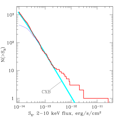
Figure 3: Cumulative log(N)–log(S) distribution of detected point-like sources, excluding several known foreground stars and rotation powered pulsars (section 3). The thin and thick histograms show, respectively, the observed distribution and the distribution corrected for the incompleteness effects, as described in section 2.3. The thick grey line shows the log(N)–log(S) of CXB sources according to Moretti et al. (2003).

3.5 Other intrinsic LMC sources

An important type of X-ray sources associated with star formation are Wolf-Rayet stars. Due to strong stellar wind with $\dot{M}_{wind}\sim 10^{-5}$–$10^{-4}$ M_☉yr^-1, a W–R star forming a binary system with another W–R or OB star can become a rather luminous X-ray source. X-ray emission in such a binary system originates from a shock formed by colliding stellar winds of its members (Cherepashchuk, 1976). Typical luminosities usually do not exceed $L_{X}\la$ few$\cdot 10^{34}$erg s^-1.

There are about 130 known W–R stars in the whole LMC. We have cross correlated our data with the fourth catalogue of W–R stars in the LMC by Breysacher et al. (1999). Four sources from our sample have been identified as W-R stars. Two of them are faint objects with fluxes $\sim$few$\cdot 10^{-14}$ erg cm^-2s^-1 identified in optics as WR+OB systems and therefore were excluded from the final source list. The other two sources, XMMUJ053844.2–690608 and XMMUJ053833.9–691157, located in 30 Dor, will be discussed in section 4.5.

Two well-known Crab-like pulsars located in the field of view of XMM-Newton observations of LMC – PSR B0540–6910 and PSR J0537–6910 – were also excluded from the final source list.

3.6 The Log(N)–Log(S) distribution

As demonstrated above, the population of compact X–ray sources in the LMC field is dominated by two types of sources – background AGNs and high mass X-ray binaries in the LMC. Their log(N)–log(S) distributions in the flux range of interest can be described by a power law with the differential slopes $\approx 2.5$ (CXB) and $\approx 1.6$ (HMXBs). Due to a significant difference in the slopes, their relative contributions depend strongly on the flux. At large fluxes, $F_{X}\ga(2-3)\cdot 10^{-13}$ erg/s/cm² ($L_{X}\ga 10^{35}$ erg/s) the X-ray binaries in LMC prevail. On the contrary, in the low flux limit, e.g. near the sensitivity limit of our survey, $F_{X}\sim 10^{-14}$ erg/s/cm², the vast majority of the X-ray sources are background AGN.

This is illustrated by Fig. 3, showing the observed and corrected for incompleteness log(N)–log(S) distribution of all sources from the final source list. The corrected log(N)–log(S) distribution agrees at low fluxes with that of CXB sources. At high fluxes, there is an apparent excess of sources above the numbers predicted by the CXB sources log(N)–log(S), due to the contribution of HMXBs.

4 Identification of HMXB candidates

To filter out contaminating background and foreground sources, we use the fact that optical emission from HMXBs is dominated by the optical companion, whose properties, such as absolute magnitudes and intrinsic colors, are sufficiently well known. The X-ray-to-optical flux ratios of HMXBs also occupy a rather well-defined range. In addition, we take into account the fact that intrinsic LMC objects have small proper motions, $\la 1-2$ mas/yr (Westerlund, 1997), which helps to reject a number of foreground stars with high proper motion.

4.1 Optical properties of HMXBs counterparts

High mass X-ray binaries are powered by accretion of mass lost from the massive early-type optical companion. The mechanism of accretion could be connected to either (i) strong stellar wind from an OB supergiant (or bright giant) or (ii) an equatorial circumstellar disk around Oe or Be type star (e.g. Corbet, 1986; van Paradijs & McClintock, 1994). Taking into account positions of possible optical counterparts on the Hertzsprung-Russel diagram, the distance modulus of the LMC, $(m-M)_{0}=18.45\pm 0.1$ (Westerlund, 1997), and foreground and intrinsic reddening towards the LMC, E(B–V)$\sim 0.1-0.2$ (Westerlund, 1997), we can estimate visual magnitudes of HMXB optical companions. OB supergiants and bright giants (luminosity classes I–II) have absolute magnitudes M${}_{V}\sim-7\div-4$, corresponding to an apparent magnitude in the range m${}_{V}\sim 11.5\div 14.5$. The position of Oe and Be stars in the H–R diagram is close to the main sequence. The majority of such systems have optical companions with a spectral class earlier than B3. Indeed, in the catalog of high mass X-ray binaries of Liu et al. (2000), in only two systems was the optical counterpart classified as B3Ve and in $\sim 4-5$ – later than B3, out of $\sim 90$ HMXBs with known optical counterparts. Therefore the absolute magnitudes of majority of Be/X binaries are brighter than $M_{V}\la-1.6({\rm B3Ve})\div-2.4({\rm B2Ve})$. This corresponds to a visual magnitude $m_{V}\la 16.0\div 16.9$ and about $\approx 0.1$ magnitude brighter in the R-band. Accounting for the interstellar extinction, $A_{V}\sim 0.3-0.6$, we conclude that the majority of HMXBs have apparent magnitudes brighter than $m_{V}\la 16.5-17.5$, $m_{R}\la 16.2-17.0$. Such magnitude filtering rejects the majority of AGN typically having fainter optical counterparts.

As potential optical counterparts of HMXBs belong to spectral classes earlier than $\sim$ B3, their intrinsic optical and near-infrared colors are constrained by $R-I\la-0.19$, $B-V\la-0.20$, $V-R\la-0.08$, $J-K\la-0.16$, $I-K\la-0.34$. Taking account of the interstellar reddening, the apparent intrinsic colors will not exceed $\la 0.1-0.2$.

The interstellar extinction is known to vary across the LMC. In the above estimates, the upper range of the usually quoted values (Westerlund, 1997) was used. A several times higher extinction is observed in the 30 Doradus region, $E(B-V)=0.3-0.6$, with the mean value in the central region $E(B-V)=0.44\pm 0.22$, and $E(B-V)=0.65$ towards the center of the nebula (Westerlund, 1997). Another complication is related to the fact that two (USNO-B and GSC) out of the three catalogs used for initial search of optical counterparts of X-ray sources (section 4.2) have “holes” with a diameter of $\sim 10\arcmin-15\arcmin$ in the 30 Doradus region. This region is considered separately in section 4.5.

The above discussion is based on our knowledge of HMXB optical counterparts in the Milky Way. The depleted metallicity in the LMC will, of course, affect the optical properties of the HMXB counterparts. From the stellar evolution studies it is known that, for LMC metallicity, the effective temperature of the early-type stars on the main sequence increases by $\sim 0.01-0.05$ dex (Schraer et al., 1993), resulting in the intrinsic colors being by $\sim 0.1-0.2$ magnitude bluer than the Galactic ones. As such, these changes do not affect the efficiency of our selection criteria. The difference in metallicity might have a more significant effect on formation of HMXB systems. These effects have not been studied yet and are one of the subjects of this paper. On the other hand, from the optical spectroscopy of 14 known HMXBs in LMC, Negueruella & Coe (2002) concluded that their overall optical properties are not very different from the observed Galactic population. This suggests that the selection criteria based on the optical properties of the Galactic HMXBs would be able to identify most of the HMXBs in the LMC, with the exception of a small fraction of peculiar objects, which in the case of the Milky Way constitute less than $\sim 5-10\%$ of the total population of HMXBs.

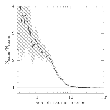
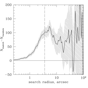
Figure 4: Left: Ratio of the actual number of matches between the X-ray source list and USNO-B catalog to the the expected number of chance coincidences, as a function of the search radius. Right: Difference between the number of matches and the expected number of chance coincidences. The vertical dashed line in both panels shows the search radius of $3.6$ arcsec. The shaded area indicates the Poisson uncertainty, computed from the square root of the actual number of matches.

4.2 Catalogs and selection criteria

We have used the following optical and near-infrared catalogs:

1. USNO-B, version 1.0 (Monet et al., 2003)

2. Guide Star Catalog, version 2.2.1 (GSC2.2.1) (Morrison & McLean, 2001)

3. The CCD survey of the Magellanic Clouds (Massey, 2002)

4. 2-micron All Sky Survey (2MASS) (Cutri et al., 2003)

5. The point source catalogue towards the Magellanic Clouds extracted from the data of the Deep Near-Infrared Survey of the Southern Sky (DENIS) (Cioni et al, 2000)

As a first step, we cross-correlated the XMM-Newton X-ray source list with the USNO-B, GSC and Massey (2002) optical catalogs, using a search radius of 3.6 arcsec and the following selection criteria: $R<17.5$, $R-I<1.5$, $B-R<1.5$ and $V-R<1.5$. If an optical object was present in the USNO-B and GSC catalogs, the preference was given to GSC, as it has a higher photometric accuracy. The color limits are significantly higher than the possible colors of HMXB optical companions and were chosen to account for the limited photometric accuracy of optical catalogues. Relaxed color limits also allow for variations of the intrinsic LMC reddening up to $E(B-V)\sim$1.5, corresponding to N${}_{H}\sim 8\cdot 10^{21}$ cm^-2. We have found optical counterparts for 78 X-ray sources. Taking into account the surface density of the optical objects in the vicinity of X-ray sources and the value of the search radius, we estimate the number of random matches to be 30, i.e. about half of all optical matches.

In the second stage, we cross-correlated all X-ray sources having optical counterparts with the near-infrared catalogs 2MASS and DENIS, using the same search radius as before. The following filtering procedure was then applied.

1. For X-ray sources with near-infrared counterparts, all those with the infrared colors J–K or I–K $>$0.7 were excluded from the following consideration.

2. All X-ray sources whose optical counterparts had detected proper motion were rejected (all such objects had proper motion $>10$ mas/yr, significantly exceeding that of the LMC).

3. If the optical counterpart was located at a distance of more than two positional errors of the X-ray source plus $1.5\arcsec$, the X-ray sources was rejected. The $1.5\arcsec$ was added to allow for the astrometric accuracy of the XMM-Newton boresight.

4. All X-ray sources with low X-ray-to-optical flux ratio $F_{X}/F_{\rm opt}<10^{-3}$ were rejected. The optical flux was calculated from the R-band magnitude using F${}_{\rm opt}=3.83\cdot 10^{-6}\cdot 10^{-m_{R}/2.5}$ erg/s/cm².

   Such low $F_{X}/F_{\rm opt}<10^{-3}$ ratios are typical for foreground stars but not for X-ray binaries. All confirmed HMXBs in our sample have $F_{X}/F_{\rm opt}>10^{-2}$, except RXJ0532.5-6551 and RXJ0520.5–6932, which have $F_{X}/F_{\rm opt}\approx 3.6\cdot 10^{-3}$ and $\approx 4.6\cdot 10^{-3}$ respectively.

5. If an optical counterpart was found also in the Massey (2002) catalogue, having high photometric accuracy, we used its optical colors for spectral classification, rejecting X-ray sources with counterparts of spectral type later than A0.

Table 3: List of HMXB candidates

#	R.A.	Dec.	$F_{X}$ (1)	$L_{X}$ (1)	$m_{R}$	$V-R$	Fx/Fopt	Comments
			erg/s/cm-2	erg s-1
Likely HMXB candidates(3)
1	05 38 56.7	-64 05 03	$2.67\cdot 10^{-11}$	$8.0\cdot 10^{36}$	16.7	-0.25	33	LMC X-3
2	05 31 13.1	-66 07 07	$3.01\cdot 10^{-12}$	$9.0\cdot 10^{35}$	14.0	0.23	0.31	Be/X EXO053109–6609
3	05 30 11.4	-65 51 23.4	$6.59\cdot 10^{-13}$	$2.0\cdot 10^{35}$	14.7	0.18	0.13	Be/X ? 272s pulsar(2)
4	05 31 15.4	-70 53 50	$5.25\cdot 10^{-13}$	$1.6\cdot 10^{35}$	13.6	0.1	0.038
5	05 41 34.7	-68 25 50	$2.04\cdot 10^{-13}$	$6.1\cdot 10^{34}$	14.0	-0.03	0.02
6	05 29 47.7	-65 56 43	$1.51\cdot 10^{-13}$	$4.5\cdot 10^{34}$	14.6	-0.02	0.027	Be/X transient RXJ0529.8–6556
7	05 32 32.5	-65 51 41	$5.93\cdot 10^{-14}$	$1.8\cdot 10^{34}$	13.4	-0.36	0.0036	OB RXJ0532.5–6551
8	05 20 29.4	-69 31 56	$4.05\cdot 10^{-14}$	$1.2\cdot 10^{34}$	14.1	0.03	0.0046	RXJ0520.5–6932
9	05 31 18.2	-66 07 30	$3.42\cdot 10^{-14}$	$1.0\cdot 10^{34}$	16.0	-1.36	0.023
Sources of uncertain nature(4)
10	05 23 00.0	-70 18 32	$7.93\cdot 10^{-14}$	$2.4\cdot 10^{34}$	17.3	0.45	0.17	M
11	05 37 17.0	-64 12 17	$6.19\cdot 10^{-14}$	$1.9\cdot 10^{34}$	17.2		0.063	GSC, N
12	05 41 23.4	-69 36 34	$5.84\cdot 10^{-14}$	$1.8\cdot 10^{34}$	17.1		0.11	C
13	04 53 11.8	-68 39 47	$5.71\cdot 10^{-14}$	$1.7\cdot 10^{34}$	16.7	0.17	0.071	C
14	05 30 02.3	-71 00 46	$5.3\cdot 10^{-14}$	$1.6\cdot 10^{34}$	14.9		0.013	USNO-B
15	05 44 34.3	-68 28 14	$4.99\cdot 10^{-14}$	$1.5\cdot 10^{34}$	17.4		0.12	USNO-B
16	05 20 13.6	-69 09 42	$4.72\cdot 10^{-14}$	$1.4\cdot 10^{34}$	16.0		0.031	M
17	05 18 03.7	-69 01 14	$3.51\cdot 10^{-14}$	$1.1\cdot 10^{34}$	17.1		0.063	USNO-B
18	05 33 46.9	-70 59 15.4	$3.46\cdot 10^{-14}$	$1.0\cdot 10^{34}$	14.4	0.93	0.0052	C
19	05 40 43.6	-64 01 45	$3.36\cdot 10^{-14}$	$1.0\cdot 10^{34}$	17.1		0.062	C
20	05 24 15.3	-70 04 35	$2.80\cdot 10^{-14}$	$8.4\cdot 10^{33}$	17.0		0.024	USNO-B
21	05 27 33.0	-65 34 47	$2.77\cdot 10^{-14}$	$8.3\cdot 10^{33}$	16.2		0.022	M
22	05 27 02.0	-70 05 16	$2.75\cdot 10^{-14}$	$8.3\cdot 10^{33}$	17.4		0.063	USNO-B
23	05 23 15.2	-70 14 38	$2.35\cdot 10^{-14}$	$7.1\cdot 10^{33}$	16.1		0.018	USNO-B
24	05 27 02.6	-67 27 28	$2.11\cdot 10^{-14}$	$6.3\cdot 10^{33}$	14.4		0.0032	USNO-B, N
25	05 21 07.6	-69 03 01	$1.66\cdot 10^{-14}$	$5.0\cdot 10^{33}$	16.4		0.016	USNO-B
26	05 27 31.5	-65 20 34	$1.58\cdot 10^{-14}$	$4.7\cdot 10^{33}$	17.3		0.034	USNO-B
27	05 26 55.5	-65 20 49	$1.41\cdot 10^{-14}$	$4.2\cdot 10^{33}$	17.5		0.037	C
28	05 25 03.6	-70 08 16	$1.37\cdot 10^{-14}$	$4.1\cdot 10^{34}$	17.4		0.033	USNO-B
30 Doradus region ($r\leq 4\arcmin$)
29	05 38 44.2	69 06 08	$8.35\cdot 10^{-13}$	$2.5\cdot 10^{35}$				Wolf-Rayet star in R136
30	05 38 41.7	69 05 14	$1.03\cdot 10^{-13}$	$3.1\cdot 10^{34}$				Wolf-Rayet star in R140

(1) – 2–10 keV band; (2) – (Haberl et al., 2003); (3) – optical counterpart is consistent with being an HMXB; (4) – the optical counterpart exists, but the information is insufficient for its reliable classification; (5) – B–V color from Liu et al. (2000); (6) – B–V color;

Comments: USNO-B – counterpart in USNO-B only; GSC – counterpart in GSC only; M – multiple non-overlapping optical and/or infrared counterparts; C – ambiguous color indexes; N – non-HMXB nature is likely;

4.3 Search radius

To choose the search radius for cross-correlation with the optical and infrared catalogs we analyzed the dependence of the number of matches between the X-ray source list and the USNO-B catalog as a function of the search radius. No magnitude or color filtering was performed for this analysis. Furthermore, for a noticeable fraction of optical objects, the USNO-B catalog contains multiple entries. No attempt to filter out such multiple entries was made (unlike for the final analysis, described in sections 4.2 and 4.4). Therefore the absolute numbers of the total number of matches and of chance coincidences should not be directly compared with the numbers in section 4.2.

At large values of the search radius, $r_{0}\ga 10\arcsec-20\arcsec$, the observed number of matches asymptotically approaches the $N_{\rm match}\propto r_{0}^{2}$ law, expected for the number of chance coincidences (Fig.4, left panel). As the localization accuracy of XMM-Newton is sufficiently high, generally better than $\sim$few arcsec, at small values of the search radius, the total number of matches is dominated by true optical counterparts of X-ray sources. As is obvious from Fig.4, the chosen value of the search radius, $r_{0}=3.6$ arcsec, allows us on one hand to detect a significant fraction, $\ga 80-90\%$, of true optical counterparts (right panel). On the other hand, it results in a reasonable fraction of chance coincidences, $\la 50-60\%$ (Fig.4, left panel).

4.4 Identification results

After the filtering, 28 X-ray sources were left in the list of potential HMXB candidates (Table 3). Of these, 9 sources have optical properties consistent with HMXB counterparts. These sources are considered likely HMXB candidates and are listed in the first half of the table. All known HMXBs located in the filed of view of the XMM-Newton observations are among these sources. Listed in the second half are the sources whose nature cannot be reliably established based on the available optical data.

Comments on the individual sources:

#9: This source has multiple counterparts in USNO and GSC catalogues. One of USNO sources has high proper motion and high F_x/F${}_{opt}\sim 10^{-2}$, therefore, it is likely a chance coincidence. Another three GSC and one USNO sources from significantly different epochs are located at nearly the same position and show no evidence of proper motion. Their color indexes have large uncertainties, but all agree with the HMXB nature of the source. It is included in the list of likely HMXB candidates, although it is less reliable than other sources in this group.

#12: This source has been previously classified by Sasaki et al. (2000) as an HMXB candidate because of the nearby B2 supergiant. However, its improved X-ray position obtained by XMM deviates by $\approx 20\arcsec$ from the proposed B2 star. This significantly exceeds the positional error of $\sigma_{r}\approx 2.7\arcsec$ making the association with the B2 supergiant improbable. The optical matches found within $3.6\arcsec$ do not allow us to reach definite conclusion about the nature of this source.

#13: The optical counterpart of this source was found in the Massey (2002) catalogue. The color indexes B–V=0.25 and $V-R=0.17$ and proper motion of the nearby USNO source do not allow us to draw conclusions about its nature.

4.5 30 Doradus region

Owing to high stellar density, the central part of this luminous HII region is not well represented in the all-sky optical catalogs, such as USNO and GSC.

There are 5 X-ray sources in the final XMM list within the nominal size of the nebula, $r\leq 7\arcmin$ (Westerlund, 1997). Of these, 3 are located outside $r\approx 4.5$ arcmin and a search for their optical counterparts does not present a problem. The remaining 2 sources, XMMUJ053844.2–690608 and XMMUJ053841.7–690514, are located at $r\leq 1\arcmin$ from the center of 30 Dor and positionally coincide with the R136 and R140 stellar clusters respectively. Both sources show evidence for non-zero angular extent in XMM data. They were detected earlier by ROSAT and were classified as high mass X-ray binaries (Wang, 1995). Based on Chandra data, Portegies Zwart et al. (2002) resolved XMMUJ053844.2–690608 into one bright source and a number of weaker sources, all positionally coincident with bright early type (O3f* or WN) stars in the R136 cluster. XMMUJ053841.7–690514 is located in the R140 stellar cluster, known to contain at least 2 WN stars. Based on the positional coincidence with Wolf-Rayet stars and, mainly, on the young age of the R136 cluster, $\la 1-2$ Myr (Massey & Hunter, 1998), insufficient to form compact objects, Portegies Zwart et al. (2002) suggested that all these sources are colliding wind Wolf-Rayet binaries, rather than HMXBs. However, for the two brightest sources the X-ray-to-bolometric flux ratios, $F_{X}/F_{\rm bol}\sim 10^{-5}$, exceed by $\sim 1-2$ orders of magnitude the typical values for such objects in the Galaxy and for other sources detected by Chandra in R136 (Portegies Zwart et al., 2002).

Because of this uncertainty we exclude from further consideration the $r\leq 4\arcmin$ region, centered on the R136 stellar cluster. We note that this does not affect our main results and conclusions.

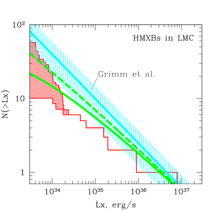
Figure 5: The incompleteness-corrected XLF of HMXB candidates in LMC. The upper histogram shows all sources from Table 3, except two in the 30 Dor region; the lower one shows likely HMXB candidates (upper part of Table 3). These two histograms provide upper and lower limits for the true HMXB XLF. The upper grey line and shaded area show the luminosity distribution predicted from the “universal” XLF of Grimm et al. (2003) extrapolated towards low luminosities and its uncertainty. The lower solid and dashed lines show the same XLF modified by the “propeller effect” assuming the black hole fraction of $f_{\rm BH}=0$ and $f_{\rm BH}=0.3$ respectively (section 6).

4.6 Completeness

The completeness of the list of HMXB candidates is defined by the following factors:

1. The completeness of the optical catalogues.

   The initial search for optical counterparts is based on the GSC2.2 and USNO-B catalogs. The GSC2.2 is a magnitude-selected ($V\leq 19.5$) subset of the GSC-II catalog (http://www-gsss.stsci.edu/gsc/gsc2/GSC2home.htm). The latter is complete to $J=21$ at high galactic latitudes (Morrison & McLean, 2001). The USNO-B 1.0 catalog is believed to be complete down to $V=21$ (Monet et al., 2003). Completeness of both catalogs is known to break down in the crowded regions. One example of such a region is the central part of 30 Dor which was excluded from the analysis (section 4.5). As no sensitivity maps for the optical catalogs exist, a quantitative estimate of the completeness of the initial counterpart search is impossible. However, the quoted completeness limits of both catalogs are $2-3.5$ mag better than chosen threshold of $17.5$ mag for the optical counterpart search. This suggests that the completeness of the optical catalogs is unlikely to be the primary limiting factor.

2. The efficiency of the initial search due to statistical and systematic uncertainties in the positions of X-ray and optical sources. This is probably one of the major limiting factors. With the chosen value of the search radius, 3.6$\arcsec$, we detect $\sim 80-90\%$ of true matches (section 4.3, Fig.4).

3. The filtering procedure applied to the optical matches found in the initial search. This procedure is based on expected optical and near-infrared properties of HMXBs and, as discussed in section 4.1, it would detect $\sim 95\%$ of HMXBs listed in the catalog of Liu et al. (2000).

Thus, we estimate the overall completeness of our HMXB sample to exceed $\ga 70-80\%$. As the latter two factors are flux-dependent, they might affect not only the total number of detected HMXBs, but also their luminosity distribution in the faint flux limit. This effect, however, is not of primary concern as a much larger uncertainty in the luminosity distribution at faint fluxes is associated with the sources of unclear nature (Fig.5).

5 HMXBs and CXB sources in the field of the LMC

5.1 The luminosity function of HMXB candidates in the LMC

The incompleteness-corrected luminosity distribution of HMXB candidates is shown in Fig. 5. The upper and lower histograms correspond to all sources from Table 3 and to the likely HMXB candidates respectively. These two histograms provide upper and lower limits for the true X-ray luminosity function of HMXBs in the observed part of the LMC. As is clear from Fig. 5, they coincide at the luminosity $L_{X}\ga(2\div 3)\cdot 10^{34}$ erg/s, with the uncertainty of the optical identifications becoming significant only at lower luminosities. We note that the upper histogram steepens at low luminosities where its slope is close to that of the CXB sources. Such behaviour indicates that a significant fraction of low luminosity sources of uncertain nature might be background AGNs.

In order to constrain the XLF parameters, we fit the data using the maximum likelihood method (Crawford et al., 1970) with a power law distribution in the range of luminosities $L_{X}\geq 2.5\cdot 10^{34}$ erg/s, where both curves coincide. We obtain best fit value for the differential slope $\alpha=1.28^{+0.26}_{-0.23}$; the normalization corresponds to $N(>10^{35}{\rm\leavevmode\nobreak\ erg/s})\approx 5$ HMXBs. As is evident from Fig.5, the slope of the luminosity distribution appears to be somewhat flatter and its normalization smaller than predicted from extrapolation of the “universal” HMXB luminosity function of Grimm et al. (2003) – $\alpha\approx 1.6$ and $N(>10^{35}{\rm\leavevmode\nobreak\ erg/s/cm^{2}})\approx 11\pm 5$ (section 3.4).

However, the XLF flattening is not statistically significant in the $L_{X}\geq 2.5\cdot 10^{34}$ erg/s luminosity range – the Kolmogorov-Smirnov probability for the universal HMXB XLF model is $\sim 40\%$. Only in the entire luminosity range of Fig. 5 is the shape of the luminosity distribution of reliable HMXB candidates (the lower histogram in Fig. 5) inconsistent with the extrapolation of the universal HMXB XLF, the Kolmogorov-Smirnov test giving the probability of $\sim 1\%$. On the other hand, the list of reliable HMXB candidates may be incomplete below $L_{X}\la(1-2)\cdot 10^{34}$ erg/s.

Due to the limited number of sources and ambiguity of their optical identifications at low luminosities, it is premature to draw a definite conclusion regarding the precise shape of the XLF below $L_{X}\la(1-2)\cdot 10^{34}$ erg/s and its consistency with the extrapolation to the low luminosities of the universal HMXB XLF of Grimm et al. (2003). We note however that the flattening of the luminosity distribution leading to the deficit of the low luminosity sources should be expected due to the “propeller effect”. As this effect and its impact on the HMXB XLF is of interest on its own, we consider it in detail in section 6.

Another factor affecting the overall normalization of the luminosity distribution – the dependence of the number of HMXBs on the stellar population age – is discussed in section 7.

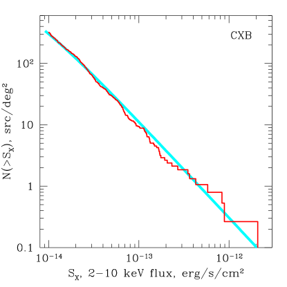
Figure 6: Cumulative logN–logS distribution of CXB sources, obtained after removal of HMXB candidates. The solid line shows the distribution from Moretti et al. (2003).

5.2 Log(N)–log(S) distribution of CXB sources

The log(N)–log(S) distribution of CXB sources obtained after removal of HMXB candidates is shown in Fig.6. The difference between the upper and lower limit on the HMXB population is insignificant in this context, due to the large number of CXB sources at low fluxes. Below we give values obtained after removing all HMXB candidates.

We fit the resulting log(N)–log(S) distribution in the flux range $F_{X}>2\cdot 10^{-14}$ erg cm^-2 s^-1 with a power law model $N(>S)=k(S/S_{0})^{-\alpha}$, where $S_{0}=2\cdot 10^{-14}$ erg/s/cm². Best fit values are $\alpha=1.62\pm 0.08$ and $k=127\pm 11$. The Kolmogorov-Smirnov test accepts this model, giving a K–S probability of $\sim 16\%$. These best fit values agree with the CXB parameters determined in other surveys, in particular with those from Moretti et al. (2003): $\alpha=1.57^{+0.1}_{-0.08}$, k=121${}^{+69}_{-31}$. The latter distribution is shown in Fig.6 by the solid line.

6 Propeller effect and HMXB XLF

6.1 The “propeller effect”

As high mass X-ray binaries are young objects, the neutron star magnetic field is sufficiently strong to be dynamically important in the vicinity of the neutron star. Indeed, the majority of known HMXBs in the Milky Way (Liu et al., 2000) and Small Magellanic Cloud (Corbet et al., 2004) are X-ray pulsars. In the presently accepted picture the transition from disk-like accretion to a magnetospheric flow, co-rotating with the neutron star, occurs in a narrow region located at the magnetospheric radius $R_{m}$. The location of the transition region is defined by the balance between the NS magnetic field pressure and the pressure (ram and thermal) of the accreting matter. There is some uncertainty in the definition of $R_{m}$, due to uncertainty in the physics of the disk–magnetosphere interaction, the canonical value being (e.g. Lamb et al., 1973):

$$R_{m}=1.4\cdot 10^{9}\,R_{6}^{10/7}M_{1.4}^{1/7}B_{12}^{4/7}\,L_{35}^{-2/7}{\rm\leavevmode\nobreak\ cm}$$ (10)

where $R_{6}$ is the neutron star (NS) radius in units of $10^{6}$ cm, $M_{1.4}$ is its mass divided by $1.4M_{\sun}$, $B_{12}$ is strength of the magnetic filed on the NS surface in units of $10^{12}$ Gauss and $L_{35}$ is X-ray luminosity in units of $10^{35}$ erg/s. It was assumed above that the mass accretion rate $\dot{M}$ is related to the X-ray luminosity via $L_{X}=(GM_{NS}/R_{NS})\dot{M}$.

The character of the disk–magnetosphere interaction depends critically on the fastness parameter, $\omega=\Omega_{*}/\Omega_{K}(R_{m})$, defined as the ratio of the neutron star spin frequency $\Omega_{*}$ and the Keplerian frequency at the magnetospheric radius $\Omega_{K}(R_{m})$. As suggested by Illarionov & Sunyaev (1975), at low mass accretion rates, the spin frequency of the neutron star can exceed the Keplerian frequency at the magnetospheric radius. In this case, corresponding to $\omega>1$, the flow of the matter towards the neutron star will be inhibited by the centrifugal force exerted by the rotating magnetosphere and the matter can be expelled from the system due to the “propeller effect”.

If the critical value of the fastness parameter $\omega_{prop}$, at which the “propeller effect” occurs, is known, the corresponding value of the critical luminosity can be computed. Using eq.(10):

$$L_{X,prop}=3.4\cdot 10^{33}\ \omega_{prop}^{-7/3}R_{6}^{5}\,M_{1.4}^{-2/3}B_{12}^{2}\,P_{100}^{-7/3}{\rm\leavevmode\nobreak\ erg/s}$$ (11)

where $P_{100}$ is the NS spin period in units of 100 sec. The value of $L_{X,prop}$ defines the lower limit on the possible X-ray luminosity of an X-ray binary with given parameters of the neutron star. At lower values of $\dot{M}$ the system will not be observable as an X-ray source. The details of the disk–magnetosphere interaction are not well understood, especially at large values of the fastness parameter. It is usually assumed that the “propeller effect” occurs at $\omega>1$. However, for the accreting matter to be expelled from the system, the linear velocity of the rotating magnetosphere should at least exceed the escape velocity, $v_{esc}=\sqrt{2}v_{K}$, which corresponds to $\omega>\sqrt{2}$. Spruit & Taam (1993) argued that, due to gas pressure effects, accretion is still possible in a narrow range $\omega\ga 1$. They suggested that the critical value of the fastness parameter is $\omega\ga\sqrt{v_{K}/c_{s}}$, where $c_{s}$ is the speed of sound at the magnetospheric radius. For a standard disk solution (Shakura & Sunyaev, 1973), this value can be very high, $\omega>>1$. On the other hand, the standard disk solution might be inapplicable in the vicinity of the magnetospheric radius (e.g. Spruit & Taam, 1993). In addition, the disk might be rather hot at the inner edge, due to dissipation of the shock, induced by the rotating magnetosphere (Illarionov & Sunyaev, 1975). Owing to the strong dependence of the luminosity on the fastness parameter (eq.(11)), this uncertainty in the critical value of $\omega$ translates into a much greater uncertainty in the value of the critical luminosity. With this in mind, we study qualitatively the impact of the propeller effect on the luminosity distribution of X-ray binaries with the neutron star primary, assuming that the propeller regime occurs at $\omega>\sqrt{2}$.

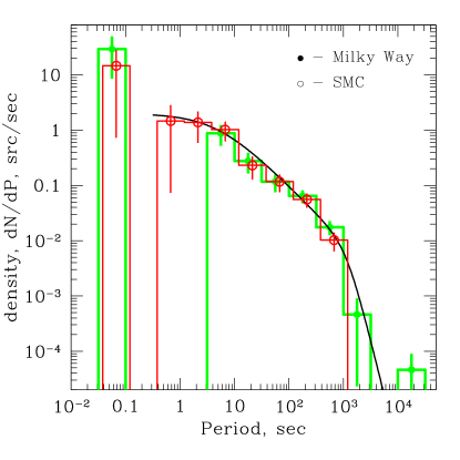
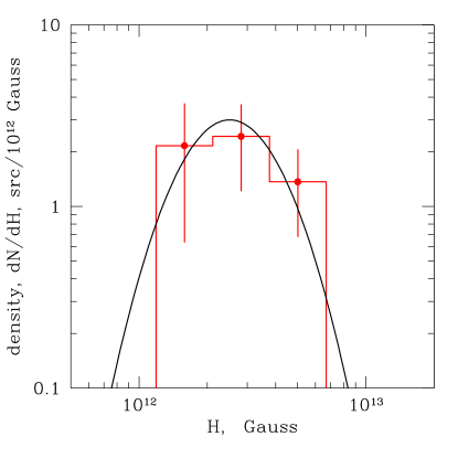
Figure 7: Distribution of spin periods (left) and magnetic field strength (right, Coburn et al. (2002)) in high mass X-ray binaries. The spin period distributions are shown separately for the Milky Way ( Liu et al. (2000)) and SMC (Corbet et al. (2004)) sources. The SMC distribution is shifted along the x axis by 0.2 dex for clarity. The smooth solid lines in both panels show the model distributions used for calculation of the propeller effect.

6.2 Impact on the HMXB luminosity distribution

The existence of the lower limit on the luminosity of an accreting neutron star will obviously modify the shape of the luminosity function of high mass X-ray binaries, leading to a deficit of low luminosity sources. The modified luminosity distribution can be calculated as:

$$\frac{dN}{dL}=\left(\frac{dN}{d\dot{M}}\right)\,\left(\frac{R_{NS}}{GM_{NS}}\right)f(L)=\left(\frac{dN}{dL}\right)_{0}f(L)$$ (12)

where the luminosity-dependent factor $f(L)$ accounts for the “propeller effect”. The undisturbed luminosity function $\left(dN/dL\right)_{0}$ is defined by the the distribution of the binary systems over the mass transfer rate $\dot{M}$ and depends on the distributions of the binary system parameters and the parameters of the optical companions in HMXBs. The function $f(L)$ is given by:

$$f(L)=\int\!\!\int\,\frac{dn}{dP}\,\frac{dn}{dB}\,\Theta(L-L_{prop}(P,B))\,dPdB$$ (13)

where $\Theta(x)$ is the Heavyside step function and $dn/dP$ and $dn/dB$ are distributions of the HMXBs over the NS spin periods and surface magnetic fields, normalized to unity. The minimal luminosity of HMXB $L_{prop}(P,B)$ is given by eq.(11), with $\omega=\sqrt{2}$ and assuming for simplicity that all neutron stars have the same mass and radius.

For the undisturbed distribution $\left(dN/dL\right)_{0}$ we extrapolated towards low luminosities the universal luminosity function of HMXBs, derived by Grimm et al. (2003):

$$\left(\frac{dN}{dL}\right)_{0}=A\,L^{-1.6}$$ (14)

As it is mainly based on the luminosity distribution of high luminosity systems, $\log(L_{X})\sim 36-40.5$, it should be relatively unaffected by the “propeller effect” and provides a reasonable approximation of the $\dot{M}$ distribution in HMXB systems.

To estimate the distributions of HMXBs over the NS spin period and magnetic field, we used the data on the known HMXBs. Strictly speaking, the observed distributions are themselves modified by the “propeller effect”, as the critical luminosity depends strongly on the NS period and magnetic field. For the purpose of this qualitative consideration we ignore this effect and use observed distributions. For the spin frequency we used the measured periods of known X-ray pulsars in the Milky Way (Liu et al., 2000) and Small Magellanic Cloud (Corbet et al., 2004). The distributions are plotted in the left panel of Fig.7, demonstrating that they are similar. We approximated these distributions with an empirical function

$$\frac{dn}{dP}=\frac{n_{0}}{1+P/5+(P/300)^{4}}\leavevmode\nobreak\ \leavevmode\nobreak\ \leavevmode\nobreak\ \leavevmode\nobreak\ \leavevmode\nobreak\ \leavevmode\nobreak\ \leavevmode\nobreak\ P_{\rm min}<P<P_{\rm max}$$ (15)

where P is the spin period in seconds and the constant $n_{0}$ is defined to normalize the distribution to unity. This approximation is shown in Fig.7 by the solid line. To estimate the $dn/dB$ distribution we use the results of the determination of the magnetic field strength from observations of the cyclotron lines by Coburn et al. (2002). The distribution is shown in the right panel in Fig.7 and was approximated by the log-Gaussian:

$$\frac{dn}{dB}=n_{0}\exp\left(\frac{(\log(B)-\log(B_{0}))^{2}}{2\sigma_{B}^{2}}\right)\leavevmode\nobreak\ \leavevmode\nobreak\ \leavevmode\nobreak\ \leavevmode\nobreak\ \leavevmode\nobreak\ \leavevmode\nobreak\ \leavevmode\nobreak\ \leavevmode\nobreak\ \leavevmode\nobreak\ \leavevmode\nobreak\ \leavevmode\nobreak\ \leavevmode\nobreak\ \leavevmode\nobreak\ \leavevmode\nobreak\ \leavevmode\nobreak\ \leavevmode\nobreak\ \leavevmode\nobreak\ \leavevmode\nobreak\ \leavevmode\nobreak\ \leavevmode\nobreak\ \leavevmode\nobreak\ \leavevmode\nobreak\ \leavevmode\nobreak\$$ (16)

$$B_{\rm min}<B<B_{\rm max}$$

with parameters $\log(B_{0})=12.4$ and $\sigma_{B}=0.2$.

The examples of the luminosity distributions, modified by the “propeller effect” for different values of the parameters are shown in Fig.8. Given the shapes of $dn/dP$ and $dn/dB$ distributions, the function $f(L)$ and resulting luminosity function weakly depend on the values of $B_{\max}\ga 10^{13}$ Gauss and $P_{\rm min}\la 0.5$ sec. Therefore they were fixed at these values. The dependence on $P_{\rm max}$ and $B_{\min}$ is significantly stronger. The long period pulsars with $P\ga 10^{3}$ sec are unaffected by the “propeller effect” but they can be subject to a significant observational bias, as the long periods are more difficult to detect. Based on the observed period distribution of the known X-ray pulsars, $P_{\rm max}\sim(1-2)\cdot 10^{3}$ sec seems to be a reasonable choice. There are no X-ray pulsars with measured $B$ below $\sim 10^{12}$ Gauss. On the other hand, for $B\sim 10^{11}-10^{12}$ Gauss, the cyclotron line energy is in the $\sim 1-10$ keV energy range, where it could have been easily detected by numerous experiments, operating in the standard X-ray band. We assumed in the following $B_{\min}=10^{12}$ Gauss.

Although the choice of $P_{max}$ and $B_{min}$ significantly affects the global shape of the luminosity function, it has a modest effect in the luminosity range of interest, $\log(L_{X})\ga 33.5$ (Fig.8). In the simplified model considered above, the shape of the luminosity function in this range is sensitive only to the radius of the neutron star and to the critical value of the fastness parameter $\omega_{prop}$ (eq.(11)).

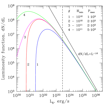
Figure 8: Impact of the propeller effect on the luminosity distribution of high mass X-ray binaries with a neutron star primary. The straight line shows the initial power law distribution with differential slope 1.6. The curved lines show the luminosity function modified by the propeller effect for different parameters of the distributions of the neutron star spin and magnetic field. The neutron star mass and radius are $M_{NS}=1.4M_{\odot}$ and $R_{NS}=13$ km. The dashed line corresponds to our sensitivity limit.

6.3 Comparison with the observed XLF

The overall impact of the “propeller effect” on the HMXB luminosity function depends on the fraction of neutron star binaries, as HMXBs with a black hole primary are, obviously, unaffected by it. Presently, there is some ambiguity in this fraction. In the Milky Way, for 50 out of 85 HMXBs, X-ray pulsations were detected (Liu et al., 2000). For only a few of the remaining 35 sources was the black hole nature of the primary confirmed. Therefore, the fraction of HMXBs with black hole primaries is $0.04\la f_{bh,MW}\la 0.45$. In the case of the Small Magellanic Cloud, there are 25 objects listed in the catalog of Liu et al. (2000), of which for 18 X-ray pulsations were detected (Liu et al., 2000; Corbet et al., 2004) and for no source was the black hole nature of the primary confirmed, therefore $f_{bh,SMC}\la 0.28$.

With this uncertainty in mind, we compare the model with the observed luminosity function of HMXBs in the LMC in Fig.5. The luminosity distributions with account taken of the “propeller effect” are shown as solid and dashed thick grey lines, computed assuming $f_{BH}=0$ and $f_{BH}=0.3$ respectively. The “propeller effect” in both curves was computed assuming $M_{NS}=1.4\leavevmode\nobreak\ M_{\sun}$, $R_{NS}=15$ km, $B_{min}=10^{12}$ Gauss, $B_{max}=10^{13}$ Gauss, $P_{min}=0.5$ sec, $P_{max}=10^{3}$ sec. The $f_{BH}=0$ curve illustrates the maximum amplitude of the impact of the “propeller effect” on the luminosity distribution of HMXBs (for the given choice of the NS parameters and $\omega_{prop}$).

As expected, the “propeller effect” results in the deficit of low luminosity sources and flattening of the XLF. This behaviour is qualitatively similar to the observed XLF (Fig.5). However, due to lack of distinct features of the “propeller effect” in the XLF at $\log(L_{X})\ga 33$ and large uncertainty in the observed HMXB XLF at low luminosities, it is premature to draw any definite conclusion regarding the relevance of the “propeller regime” of accretion onto a strongly magnetized neutron star. Its impact would be more apparent in the $\log(L_{X})\la 32$ luminosity range. In order to construct this, a larger number of sources and better sensitivity limits are required.

7 HMXBs and the age of underlying stellar population

7.1 Spatial distribution of HMXBs in LMC

Considered globally, the number and luminosity distribution of HMXBs in the observed part of the LMC roughly agree with expectation based on the universal luminosity function of HMXBs, probably modified by the propeller effect at the low luminosity end (Fig.5). However, examination of the numbers of detected HMXBs in the individual XMM pointings reveals a significant non-uniformity of the $N_{HMXB}/SFR$ ratio, as illustrated by Fig.9. This figure also shows all known HMXBs and HMXB candidates in LMC. These do not represent a flux-limited sample, therefore, it should be interpreted with caution. Nevertheless, their spatial distribution shows the same trends as the distribution of the HMXBs detected by XMM, which do constitute a flux-limited sample. Fig.9 reveals the remarkable absence of correlation between the surface density of HMXBs and the star formation rate, as traced by $H_{\alpha}$ emission. Indeed, nearly half of the known HMXBs are located in the north-east part of the supergiant shell LMC 4 and beyond it. On the other hand, there are only a few HMXBs in and near the 30 Dor region, which has the highest surface density of star formation, as traced by $H_{\alpha}$ and FIR emission, and accounts for $\approx 50\%$ of the total SFR in the part of the LMC covered by the survey. Factors such as obscuration and the SN kicks do affect the spatial distribution of HMXBs, but they seem to be insufficient to explain the observed distribution. Indeed, the largest interstellar extinction in the LMC region is observed towards the center of 30 Dor, $E(B-V)=0.65$ (Westerlund, 1997), corresponding to the hydrogen column density of $N_{H}\approx 3.5\cdot 10^{21}$ cm^-2. This value cannot affect the spatial distribution of the sources in the 2–8 keV band in any significant way. The typical SN kick velocities of HMXBs are unlikely to exceed $\sim 50$ km/s, which corresponds to $\sim 3.5$ arcmin/Myr at the LMC distance. Such a velocity is obviously insufficient to significantly modify the HMXB spatial distribution on the angular scale of degrees over a few million years. A more attractive explanation is offered by the effects related to the age of the underlying stellar population, as discussed below.

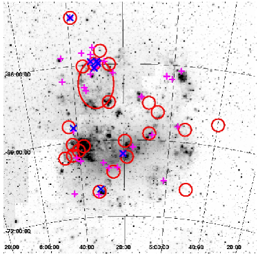
Figure 9: The $H_{\alpha}$ map of LMC (greyscale image). The overlayed symbols are: “+”(magenta) – all known HMXBs from the catalog of Liu et al. (2000) and HMXB candidates discovered by ROSAT (Kahabka, 2002); “x” (blue) – likely HMXB candidates (upper part of Table 3). Large circles indicate fields of view of XMM observations. The oval-shaped region in the north-east shows the location of the LMC 4 supergiant shell. The region of the highest surface brightness, located to the south of Dec$=-69\degr$, is the 30 Doradus HII region.

7.2 HMXBs and the stellar age

HMXBs are often considered as an “instantaneous” tracer of star formation. However, the lifetime of the most massive stars of $M\sim 125\leavevmode\nobreak\ M_{\odot}$ is $\sim 2.6$ Myr and can be as long as $\sim 15-20$ Myr for $M\sim 8-10\leavevmode\nobreak\ M_{\odot}$ stars. To this time one should add a delay required for the binary to reach the HMXB phase, $\tau_{PSN}\sim 1$ Myr. Following an instantaneous creation of stars at $\tau=0$, the number of HMXBs $N_{HMXB}(\tau)$ is a non-monotonic function of time $\tau$ passed since the star formation event. It equals zero at $\tau\approx 1-3$ Myr, unless stars are formed significantly heavier than the conventionally accepted upper mass limit of $\sim 125\leavevmode\nobreak\ M_{\odot}$. At later times, the $N_{HMXB}(\tau)$ is an increasing function of $\tau$, until at least $\tau\sim 20$ Myr, corresponding to the lifetime of the least massive stars, $M\sim 8\leavevmode\nobreak\ M_{\sun}$, capable of leaving behind a compact object. The behaviour of $N_{HMXB}(\tau)$ at later times is not clear. One might expect that at $\tau\ga 20$ Myr, the number of HMXBs will decrease with time. However, this behaviour will be affected by the binary systems with a less massive companion, entering the HMXB phase at later times (i.e. having a longer time delay $\tau_{PSN}$).

This simple picture might qualitatively explain the observed non-uniformity of the spatial distribution of HMXBs in the LMC. Indeed, the central region of 30 Dor has a very young age, $\approx 1-2$ Myr, as revealed by its H-R diagram and stellar mass distribution (Massey & Hunter, 1998). This is insufficient to form compact objects – neutron stars or black holes, as was noted by Portegies Zwart et al. (2002), unless stars with masses exceeding $\sim 150\leavevmode\nobreak\ M_{\odot}$ were formed in R136. The LMC4 supergiant shell, on the other hand, has an age of $\sim 10$ Myr (Braun et al., 1997), which is sufficient for all stars heavier than $\sim 20\leavevmode\nobreak\ M_{\sun}$ to have become collapsed objects. The OB associations in the southern part of LMC 4 are somewhat younger, with ages ranging from $\sim 2$ Myr to $\sim 6-9$ Myr (Braun et al., 1997, and references therein), which might explain the pausity of HMXBs there.

In the bow-shock induced star formation model of de Boer et al. (1998), the stellar population age increases clockwise from $\la 1$ Myr to the south-east of 30 Dor, to $\sim 10-15$ Myr in the north-east of the LMC, near LMC 4, to $\sim 20-40$ Myr to the north-west. This also qualitatively agrees with the observed distribution of HMXBs in the LMC.

7.3 Number of HMXBs as a function of time after the star formation event

The proximity of LMC allows to construct H-R diagrams and sufficiently accurately determine the age and the mass function of the stellar population in various parts of LMC. Due to the small inclination angle and, consequently, small depth, the individual stellar associations can be studied without significant projection effects and contamination by the foreground and background populations. As a result of these studies, it has been found that the supergiant shells in the LMC often host coeval stellar populations. One of the most intriguing examples is the LMC 4 supergiant shell, with a diameter of $\sim 1.4$ kpc, inside which no significant age gradients have been found, with all the stars having approximately the same age of $\sim 9-12$ Myr (Braun et al., 1997). X-ray observations and HMXB number-counts in the fields, well studied in the optical band, open a unique possibility to directly determine the number of high mass X-ray binaries as a function of time elapsed since the star formation event. This possibility is explored below using two stellar associations in the LMC as an example – the R136 stellar cluster and the northern part of the LMC 4 supergiant shell.

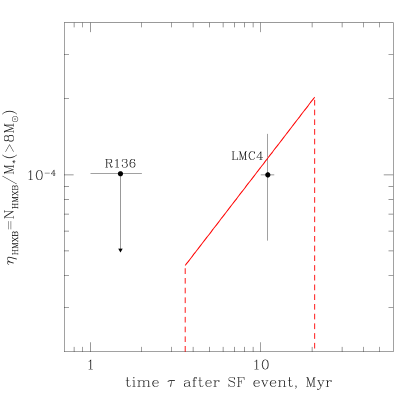
Figure 10: The time dependence of the specific number of HMXBs, $\eta_{HMXB}(\tau)$. The point with error bars and the upper limit are data on the LMC 4 supergiant shell and R136 star cluster (Table 4). The solid line shows the simple model described in section 7.3 with the normalization determined from the $N_{HMXB}-$SFR relation from Grimm et al. (2003).

We assume that stars are formed instantaneously at time $\tau=0$ with the Salpeter IMF with an upper mass cut-off $M_{u}=125\leavevmode\nobreak\ M_{\sun}$. The time-dependent specific number of HMXBs, $\eta_{HMXB}(\tau)$, is defined as the number of HMXBs present after time $\tau$ since the star formation event, normalized to the total mass of massive stars with $M\geq 8\leavevmode\nobreak\ M_{\sun}$, formed at $\tau=0$:

$$\eta_{HMXB}(\tau)=\frac{N_{HMXB}(\tau)}{M(>8M_{\sun}\,,\tau=0)}$$ (17)

The age of the stellar population in the northern part of LMC 4 was determined by Braun et al. (1997) from the analysis of the H-R diagram, $\tau\approx 10-12$ Myr, with little dispersion between individual fields. Braun et al. (1997) also determined the stellar mass function and have shown that its slope in the $\sim 3-15\leavevmode\nobreak\ M_{\sun}$ range is close to the Salpeter value of 2.35. The surface mass density of the initially-formed massive stars with masses between 8 and 125 $M_{\sun}$ is $\approx 85\leavevmode\nobreak\ M_{\sun}/{\rm arcmin}^{2}$. Extrapolating these results to the XMM observation of the LMC Deep field, covering $\approx 600$ arcmin² and whose FOV did not coincide with the fields studied by Braun et al. (1997) but was almost within the boundaries of LMC 4, we can estimate the total mass of massive stars within the XMM FOV, formed $\approx 10-12$ Myr ago, $M(>8M_{\sun}\,,\tau=0)\sim 5\cdot 10^{4}\leavevmode\nobreak\ M_{\sun}$. In this observation, 5 HMXB candidates with luminosity $L_{X}\geq 10^{34}$ erg/s were detected. With these numbers we estimate

$$\eta_{HMXB}(\tau=10-12{\rm Myr})\sim 1\cdot 10^{-4}{\rm\leavevmode\nobreak\ \leavevmode\nobreak\ HMXB}/M_{\sun}.$$ (18)

A similar estimate can be made for the R136 region. For the R136 cluster we complimented the results of Massey & Hunter (1998) with the flanking fields data of Sirianni et al. (2000), covering an area of $4.9$ arcmin² centered on the R136 stellar cluster. In this region only two X-ray sources were detected by XMM, as discussed in section 4.5. As their nature is uncertain, we assume conservatively that the total number of HMXBs in this region is $\leq 2$. The results are summarized in Table 4 and plotted in Fig.10.

In a simple ad hoc model of the formation of HMXBs, the dependence $\eta_{HMXB}(\tau)$ can be estimated as follows. Braun et al. (1997), fitting the stellar tracks of Schraer et al. (1993), have found that the lifetime of a star of mass M is

$$t_{*}\approx 86\,M^{-0.72}{\rm\leavevmode\nobreak\ Myr}$$ (19)

where the mass of the star $M$ is expressed in solar units. For a Salpeter mass function, the rate of type II supernovae depends on the time $\tau$ elapsed since the star formation event as follows:

$$\frac{dN_{SN}}{dt}\propto\tau^{0.88},\leavevmode\nobreak\ \leavevmode\nobreak\ 2.6\leq\tau\leq 19{\rm\leavevmode\nobreak\ Myr}.$$ (20)

In the latter inequality $\tau=2.6$ and 19 Myr are the lifetimes of the most massive stars and of the stars with $M=8\leavevmode\nobreak\ M_{\sun}$ respectively. Taking into account that the HMXB lifetime $\tau_{H}$ is short, we obtain for the number of HMXBs active at time $\tau$:

$$N_{HMXB}(\tau)\propto\frac{dN_{SN}}{dt}(\tau-\tau_{PSN})\cdot\tau_{H}$$ (21)

where $\tau_{PSN}$ is the post-supernova time required for the binary to reach the HMXB phase. Here we have assumed that $\tau_{PSN}$ and $\tau_{H}$ are the same for all binaries. With eq.(20) we obtain:

$$\eta_{HMXB}(\tau)\propto(\tau-\tau_{PSN})^{0.88}.$$ (22)

This equation is valid for $2.6\leq\tau-\tau_{PSN}\leq 19$ Myr. The behaviour of $\eta_{HMXB}(\tau)$ outside this interval, especially at larger $\tau$, is unclear, as discussed in section 7.2. The shape of $\eta_{HMXB}(\tau)$ calculated using eq. 22 with $\tau_{PSN}=1$ Myr is shown in Fig.10.

The normalization in equation (22) depends on a number of parameters of the binary evolution, such as the total fraction of the binaries, the fraction, survived the supernova explosion etc, whose values are unknown. On the other hand, normalisation can be determined from the calibration of the $N_{HMXB}$–SFR relation obtained by Grimm et al. (2003). From its derivation, this calibration corresponds to the case of a steady star formation on a time scale longer than HMXB formation and life times. Therefore:

$$\frac{N_{HMXB}}{SFR}=\int\eta_{HMXB}(\tau)\,d\tau.$$ (23)

The normalization of the curve shown in Fig.10 was obtained from integration of eq.(23) with $\eta_{HMXB}(\tau)$ defined by eq.(22) and the integration limits 2.6 and 19 Myr. The ratio $N_{HMXB}/{\rm SFR}=N_{HMXB}(\geq 10^{34}{\rm\leavevmode\nobreak\ erg/s})/{\rm SFR}\approx 1.9\cdot 10^{3}$ was calculated using eq.(7) from Grimm et al. (2003) for HMXBs with $L_{X}>10^{34}$erg/s. As can be seen from Fig.10, within the accuracy of our (very crude) approximation, there is a good agreement with the data.

Table 4: Constraints on $\eta_{HMXB}(\tau)$

Name	Age, Myr	$M_{*}^{(1)}$	$N_{HMXB}^{(2)}$	$\eta_{HMXB}^{(3)}$
R136	$\approx 1-2$	$2\cdot 10^{4}$	$\leq 2$	$\leq 1\cdot 10^{-4}$
LMC 4	$\approx 10-12$	$5\cdot 10^{4}$	$5$	$(1\pm 0.45)\cdot 10^{-4}$

(1) – Total mass of massive stars, $M\geq 8\leavevmode\nobreak\ M_{\sun}$; (2) – number of HMXBs detected by XMM; (3) – number of HMXBs per unit stellar mass; References for age and IMF: R136 – Massey & Hunter (1998) and Sirianni et al. (2000), LMC 4 – Braun et al. (1997)

The above model is of course very simplified. In its more realistic version the effects of spread in $\tau_{PSN}$, $\tau_{HMXB}$ and in ages of the stellar population should be taken into account. However, to a first approximation such effects will only smooth the edges, leaving the overall behaviour of $\eta_{HMXB}(\tau)$ unchanged. Significantly more important are the effects of evolution of the secondary and contribution of the intermediate mass systems.

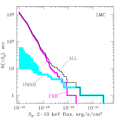
Figure 11: The log(N)-log(S) distribution of X-ray sources in the LMC field. The different histograms show the distribution of all sources, high mass X-ray binaries and CXB sources. The shaded area in the distribution of HMXBs corresponds to the range of uncertainties discussed in section 5.1.

8 Summary

Based on the archival data of XMM–Newton observations, we studied the population of compact sources in the field of the LMC. The total area of the survey is $\approx 3.8$ sq.degr. with a limiting sensitivity of $\sim 10^{-14}$ erg/s/cm² (Fig.2), corresponding to the luminosity of $\sim 3\cdot 10^{33}$ erg/s at the LMC distance.

1. Out of the 460 compact sources detected in the 2–8 keV energy band the vast majority, $\ga 94\%$, are CXB sources, observed through the LMC (section 3.1, Figs.3,11).

2. Based on the stellar mass and the star formation rate of the LMC we demonstrate that the majority, $\ga 75-90\%$, of the intrinsic LMC sources detected in the 2–8 keV band are high mass X-ray binaries (section 3).

3. The proximity of the LMC and the adequate angular resolution of XMM–Newton make it possible to reliably filter out the sources whose properties are inconsistent with being an HMXB. Based on the optical and infrared magnitudes and colors of the optical counterparts of the X-ray sources we identify 9 likely HMXB candidates (6 of which were previously known HMXBs or HMXB candidates) and 19 sources of uncertain nature (section 4, Table 3). The remaining $\sim 440$ sources, with a few exceptions, are background objects, constituting the resolved part of CXB. Their flux distribution is consistent with other determinations of the CXB log(N)–log(S) (section 5.2, Fig.6).

4. With these results we constrain lower and upper bounds of the luminosity distribution of HMXBs in the observed part of the LMC. We compare these with the extrapolation towards low luminosities of the universal luminosity function of HMXBs, derived by Grimm et al. (2003). At the high luminosity end, the observed distribution is consistent with the extrapolation of the universal XLF. The number of bright, $L_{X}\geq 10^{38}$ erg/s, “historical” HMXBs in the LMC also agrees with the value predicted from its global star formation rate. At lower luminosities, a deficit of sources is observed – the luminosity distribution seems to be somewhat flatter than the universal XLF (section 5.1, Fig.5).

5. We consider the impact of the “propeller effect” on the luminosity distribution of HMXBs (section 6, Fig.8) and demonstrate that it can explain qualitatively the observed flattening of the XLF at low luminosities (Fig.5). We note, however, that due to the relatively small number of HMXB candidates in the observed part of the LMC and the lack of distinct signatures of the “propeller effect” in the $\lg(L_{X})\ga 33$ luminosity domain (Fig.8), it is premature to draw a definite conclusion about the relevance of the “propeller regime” to the accretion onto a strongly magnetized neutron star.

6. We found significant field-to-field variations in the number of HMXBs, which appear to be uncorrelated with the star formation rates inferred by FIR and $H_{\alpha}$ emission (Fig.9). We suggest that these variations are related to different ages of the underlying stellar population in different XMM-Newton fields. Using the existence of large coeval stellar aggregates in the LMC we constrain the number of HMXBs per unit stellar mass as a function of time elapsed since the star formation event (section 7, Fig.10). Based on a simple ad hoc model, we obtain the theoretical dependence $\eta_{HMXB}(\tau)$ and show that its normalization, as constrained by the LMC data, is consistent with the calibration of the $N_{HMXB}$–SFR relation, derived by Grimm et al. (2003).