The relation between galaxy activity and the dynamics of compact groups of galaxies

Abstract

Using a sample of 91 galaxies distributed over 27 Compact Groups of Galaxies (CGs), we define an index that allows us to quantify their level of activity, be it AGN or star formation. By combining the mean activity index with the mean morphological type of the galaxies in a group we are able to quantify the evolutionary state of the groups. We find that they span a sequence in evolution, which is correlated with the spatial configuration of the galaxies making up a CG. We distinguish three main configuration Types, A, B and C. Type A CGs show predominantly low velocity dispersions and are rich in late-type spirals that are active in terms of star formation or harbor an AGN. Type B groups have intermediate velocity dispersions and contain a large fraction of interacting or merging galaxies. Type C is formed by CGs with high velocity dispersions, which are dominated by elliptical galaxies that show no activity. We suggest that the level of evolution increases in the sense A$\Rightarrow$B$\Rightarrow$C. Mapping the groups with different evolution levels in a diagram of radius versus velocity dispersion does not reveal the pattern expected based on the conventional fast merger model for CGs, which predicts a direct relation between these two parameters. Instead, we observe a trend that goes contrary to expectation: the level of evolution of a group increases with velocity dispersion. This trend seems to be related to the masses of the structures in which CGs are embedded. In general, the level of evolution of a group increases with the mass of the structure. This suggests either that galaxies evolve more rapidly in massive structures or that the formation of CGs embedded in massive structures predated the formation of CGs associated with lower mass systems. Our observations are consistent with the formation of structures as predicted by the CDM model (or $\Lambda$CDM), assuming the formation of galaxies is a biased process.

1 Introduction

Although it seems today an inescapable conclusion that the formation and evolution of galaxies is influenced by their environment, the details of how these processes occur in space and time are still largely unknown. One example is that of compact groups of galaxies (CGs). As a result of our studies of the activity in galaxies in CGs, we now have a better understanding of the evolution of galaxies in these systems (Coziol et al. 1998a,b; Coziol, Iovino & de Carvalho 2000). Our observations showed emission-line galaxies to be remarkably frequent, representing more than 50% of the galaxies in Compact Groups. Non-thermal activity, in the form of Seyfert 2s, LINERs and numerous Low Luminosity AGNs (LLAGNs; see Coziol et al. 1998a for a definition of this activity type in CGs), was found to constitute one important aspect of this activity, whereas nuclear star formation, although mildly enhanced in some groups, was noted to be generally declining. These observations were considered to be consistent with the effects of tidal forces exerted on disk galaxies when they fall into the potential well of a rich cluster or group of galaxies (Coziol, Iovino & de Carvalho 2000). Tidal stripping will remove gas from a galaxy, reducing star formation in the disk, whereas tidal triggering will start a short burst of star formation in the nuclear region and fuel an AGN (Merritt 1983, 1984; Byrd & Valtonen 1990; Henrikson & Byrd 1996; Fujita 1998).

The above processes may also produce the density-morphology-activity relation observed in CGs (Coziol et al. 1998a). By losing their gas and forming new stars near their nucleus, increasing their bulge, the morphology of spiral galaxies falling into groups is transformed to an earlier type. Assuming that groups are continuously replenished by spiral galaxies from the field (Governato, Tozzi & Cavaliere 1996; Coziol, Iovino & de Carvalho 2000), the cores of the groups are naturally expected to be populated by quiescent galaxies and AGNs (LLAGNs included), all having an early-type morphology, and their periphery to be richer in late-type star forming galaxies.

What is missing in the above description is a connection between galaxy evolution and the physical processes responsible for the formation and evolution of CGs. Our first interpretation of these systems, based on galaxy-galaxy interaction models, suggested they could not survive mergers over a long period of time (Barnes  1989), which seems in conflict with the high number of CGs observed today (for a different point of view, see Aceves & Velázquez 2002). It was then realized that this paradox may be explained, in part, by the fairly simplistic assumptions made about the nature of these systems. For example, if CGs are associated with larger and dynamically more complex structures, as many redshift surveys suggest (Rood & Strubble 1994; Ramella et al. 1994; Garcia 1995; Ribeiro et al. 1998; Barton, de Carvalho & Geller 1998), their formation and evolution must also be more complicated than previously thought.

In this study, we examine further the question of the formation and evolution of CGs, by extending our analysis of the activity to a larger sample of Hickson Compact Groups of galaxies (HCGs: Hickson 1982).

2 Observation

Long-slit spectra of 65 galaxies in 19 HCGs were obtained with the 2.1m telescope located at San Pedro Mártir, in Baja California, during one run of 4 nights in April and another of 5 nights in October 2002. A Boller & Chivens spectrograph was used in conjunction with a SITE $1024\times 1024$ CCD, yielding a plate scale of 1.05 arcsec per pixel. During the observations, the slit width was kept open to 240 micron, which corresponds to 3.1 arcsec on the sky. This aperture was chosen to be slightly larger than the effective seeing of 2 arcsec (which includes dome seeing and instrument response). We used a 300 l/mm grating, blazed at 5000 Å, which, with the slit width adopted, yielded an average resolution of 8 Å over a 4096 Å range.

Table 1 shows an excerpt of our observation logbook. Column 1 gives the date of observation, whereas column 2 identifies the object (HCG numbers and letters, as given by Hickson (1982) and as archived in CatalogVII/213 at the “Centre de Données astronomiques de Strasbourg” (CDS)). The positions of the galaxies observed in column 3 and 4 are those given in the CDS catalog, precessed by us for the year 2000. The heliocentric velocities, column 5, and the morphologies of the observed galaxies, columns 6 and 7, were also taken from the same source. Only galaxies pertaining to the groups (based on their redshifts) were observed. Note that, due to observational constraints, we did not succeed in observing all galaxies in each group, as originally planned. Our sample is therefore somewhat incomplete and biased towards the most luminous galaxies in each group. The effect this bias might have on our analysis is discussed at length in Section 4.3.

Column 8 of Table 1 gives the number of exposures and their durations. In general, we took three spectra of 900s each. The long slit (covering 322 arcsec on the sky) was always centered on the most luminous part of the galaxies and usually aligned in the E–W direction, to minimize errors introduced by guiding. In very few cases, the slit was rotated to a different angle to put more than one galaxy in the slit. These cases are identified by a plus sign in front of the HCG number of the galaxy. The effective airmass is given in the last column. Most of the observations were performed under low airmass condition, minimizing differential diffraction.

Before the first exposure, and after each of the subsequent ones, a He-Ar lamp was observed for wavelength calibration. During each night between two and three standard stars were observed to flux calibrate the spectra. During our observations we noted the frequent passage of light clouds during the night or the presence of cirrus at the beginning or end of the night, which suggests that the conditions were not photometric. Absolute flux calibration, however, is not critical for our analysis.

3 Results

3.1 Reduction and template subtraction

Standard reduction techniques were followed using IRAF. After bias subtraction, the spectra were divided by a normalized dome flat. The sky was subtracted before reducing the spectra to one dimension. After calibrating the one-dimensional spectra in wavelength, the spectra were flux calibrated. The uncertainty in the flux calibration is estimated to be 10%. For each galaxy, an average spectrum was obtained by combining the complete set of one-dimensional spectra (usually three) available for that object.

The apertures used for the reduction to one dimensional spectra contain 99% of the light from the most luminous part of the galaxies (the nucleus). The equivalent linear size for the spatial apertures (Ap.) used are listed in Table 2. It is interesting to note how compact the light distribution is in all these galaxies. For the emission-line galaxies in particular, such compactness suggests that the ionized gas covers regions extending out to only a few kpc around the nucleus (the only exception being HCG 56a). A comparison with the H$\alpha$ imaging study performed by Severgnini et al. (1999), which lists the isophotal fluxes and luminosities of H$\alpha+$NII in an area 1 $\sigma$ above the background for a sample of 73 HCGs, suggests that our spectroscopic survey may have missed at most a few regions of low star formation activity in the disk of some galaxies. Such type of activity does not seem to be predominant in CGs.

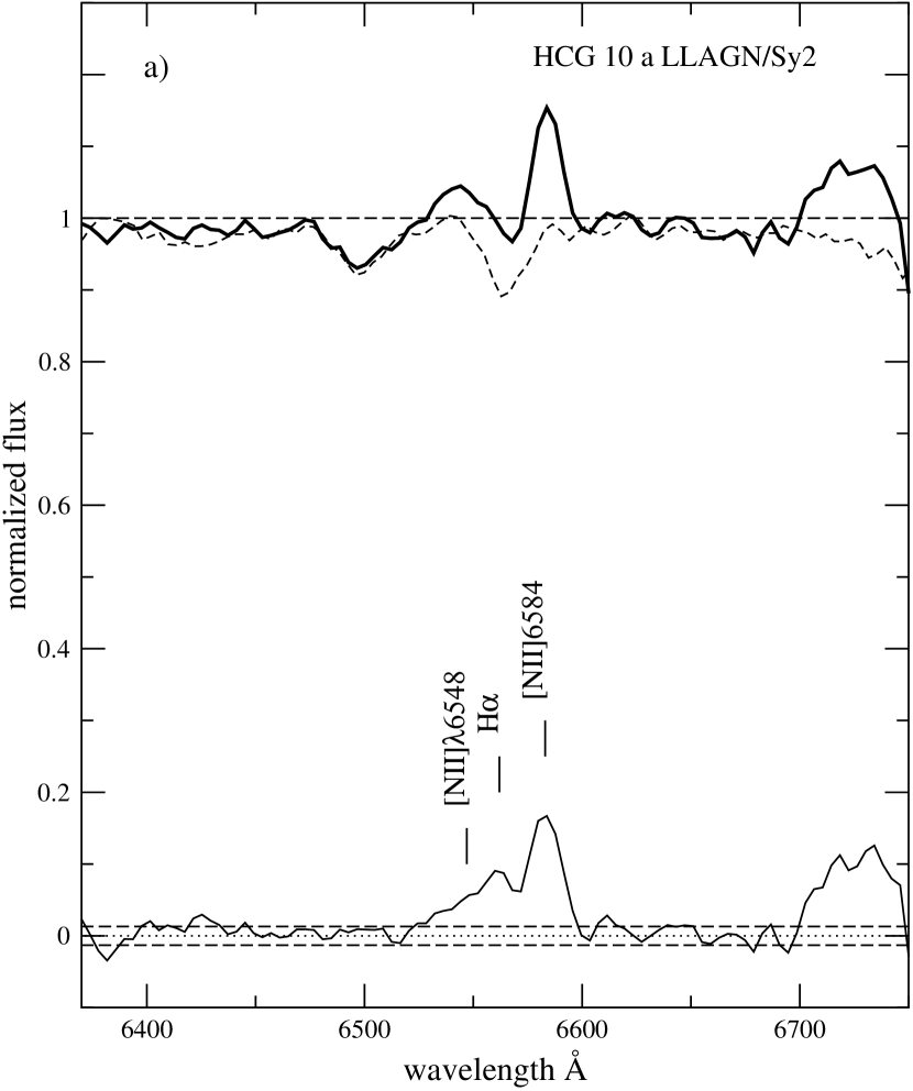
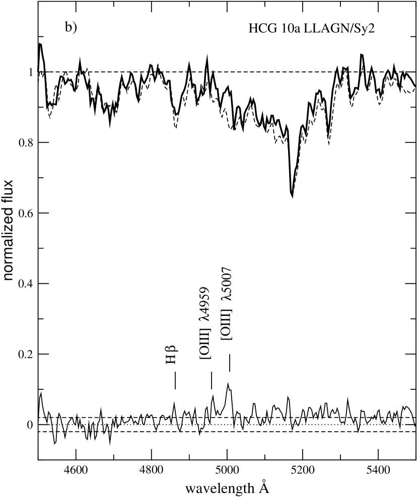
Figure 1: Examples of template subtraction in (a) the H$\alpha$ and (b) the H$\beta$ regions. The galaxy is the LLAGN candidate HCG10a. The top of the figures shows the normalized spectra before subtraction (solid line: object; dashed line: the template). The bottom of the figures shows the residual spectra after subtraction of the template, with the zero level (dotted) and $\pm 1\sigma$ rms (dashed) indicated.

Some 75% of the emission-line galaxies in the groups show strong Balmer absorption lines which needs to be corrected for before measuring line ratios in these galaxies. To accomplish this we subtracted four different templates, using the following quiescent galaxies from our sample: HCG 10b, 15c, 30a and 58d. Since we are interested only in classifying the galaxies, we did not try to fit the templates to the entire candidate galaxy spectrum. Instead, we concentrated on obtaining a good fit for the Balmer lines. The method followed is straightforward and easy to apply. First, all spectra are corrected to zero redshift. Then a region 400 Å wide around H$\alpha$ and 1500 Å wide around H$\beta$ is selected, to fit the continuum on each side of the lines. Note that a larger wavelength range is needed for H$\beta$ in order to bridge the strong Mg absorption bands visible in this region of the spectrum. Each spectrum is then normalized, dividing it by the fitted continuum. The templates, which were normalized the same way, are then simply subtracted from the candidate galaxies. One example of a template subtraction is shown in Figure 1.

The emission lines are measured in the template–subtracted spectrum by integrating the flux under the lines. For H$\alpha$, the IRAF deblend routine in SPLOT was used to correct for any contribution from [NII]. We only determined line fluxes in those cases where after template subtraction the line flux is larger than the rms in the residual (at full resolution). The H$\alpha$ flux is usually higher than 3$\sigma$ and it is higher than or equal to 2$\sigma$ for H$\beta$. In 10 cases only one of the lines (mostly H$\alpha$) was detected after template subtraction. For the line ratios, we calculated the mean of four values measured after subtracting one by one each of the individual four templates. We adopted the dispersion of the mean as the uncertainty. The two most important line ratios [NII]/H$\alpha$ and [OIII]/H$\beta$ are given in Table 2. A plus sign in front of the HCG number identifies the few emission-line galaxies for which a template subtraction was not deemed necessary, as visual inspection of the spectra did not show any signs of underlying absorption. Note that we did not apply any correction for dust extinction, since these two line ratios are known to be insensitive to this (Veilleux & Osterbrock 1987). In Table 2, we also give the H$\alpha$ luminosity and equivalent width (EW) of the H$\alpha+$[NII] lines as measured in the template subtracted spectra. The uncertainty for the luminosity is of the order of 10%. Luminosities with uncertainties larger than 20% are identified by a colon (uncertainties are always smaller than 30%). The uncertainty on the EW, which is mainly due to the template subtraction, is of the order of 1 Å.

3.2 Activity classification

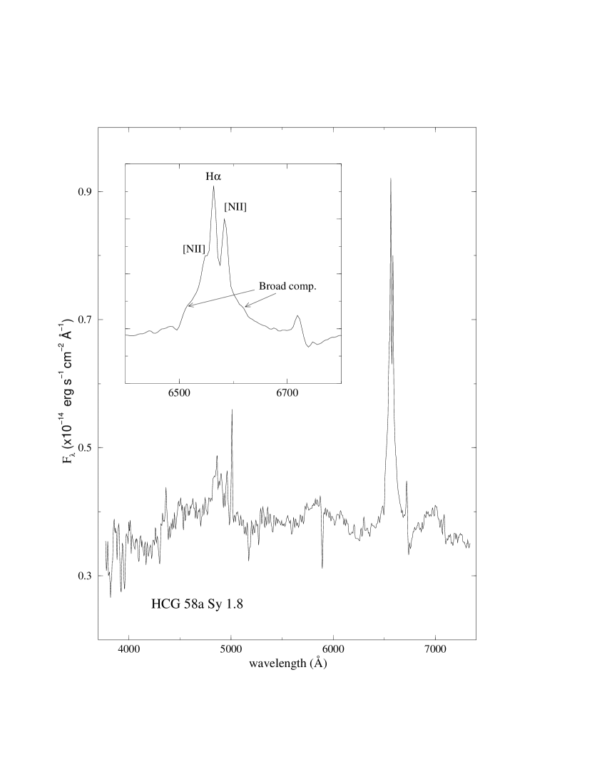
Figure 2: Optical spectrum of HCG 58a, presented in its restframe. This galaxy looks like a Seyfert 2, but the presence of large wings around H$\beta$ (already evident in the spectrum) and H$\alpha$ (evident in the enlarged section) make it a Seyfert 1.8.

Figure 2 shows the final spectrum for the galaxy HCG 58a, which is the most active galaxy in our sample. As can be seen in the enlarged region, the presence of weak, broad components around H$\alpha$ (also visible around H$\beta$) suggests this is a Seyfert 1.8 (Osterbrock 1981). We emphasize that HCG 58a is the first Seyfert 1 galaxy (although of an intermediate type) that we have found thus far, after classifying 118 galaxies in 34 HCGs. This result confirms the rarity of luminous AGNs observed in CGs (Coziol et al. 1998a; Coziol, Iovino & de Carvalho 2000).

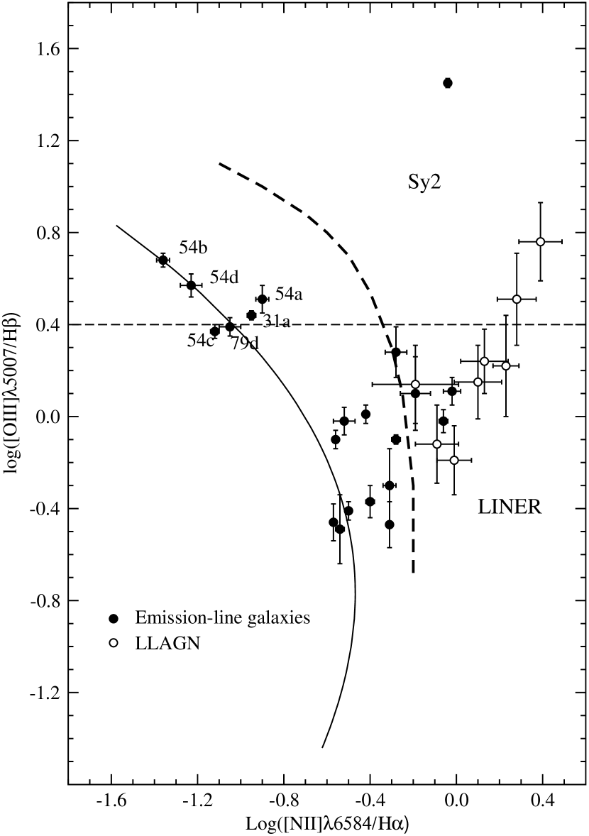
Figure 3: Standard diagnostic diagram for the emission-line galaxies in our sample. The dashed curve separates thermal (left) from non-thermal (right) galaxies, while the continuous curve is the locus traced by normal HII regions. The horizontal dashed line separates low excitation, high metallicity star forming galaxies (bottom) from high excitation, low metallicity star forming galaxies (top).

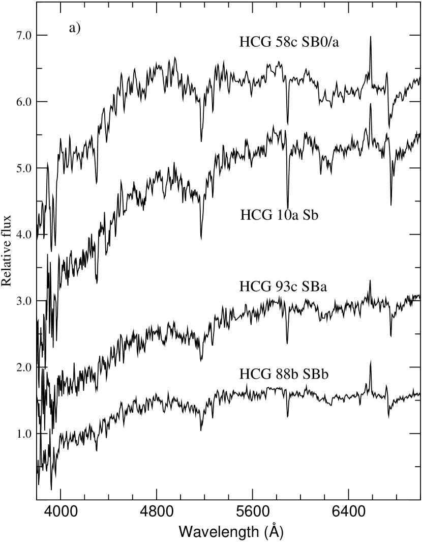
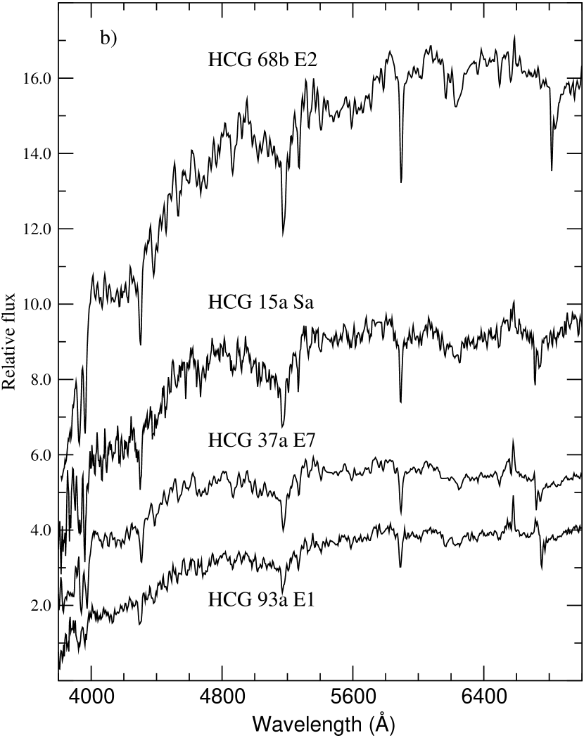
Figure 4: Spectra of the confirmed LLAGNs in our sample. All spectra are in the restframe, and slightly shifted in flux to facilitate comparison. Note the weakness of the H$\alpha$ line in emission compared to the two [NII] lines.

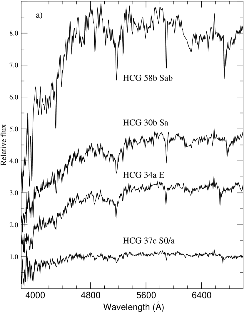
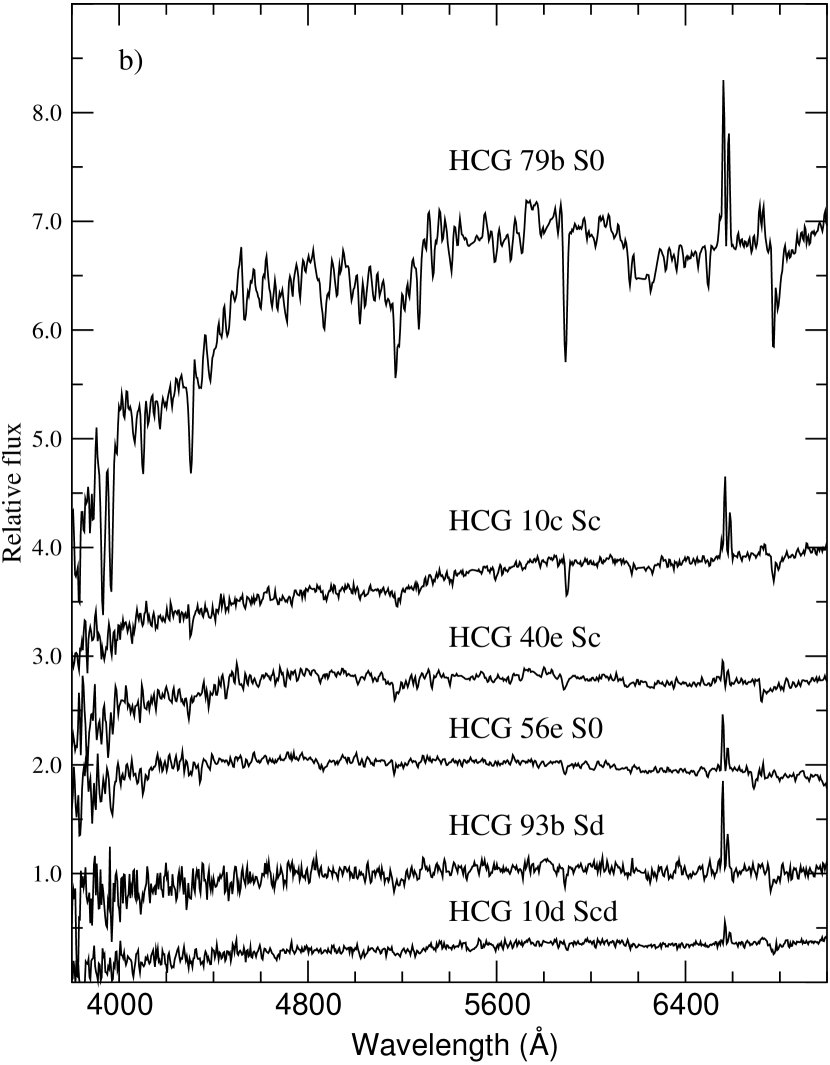
Figure 5: a) Spectra of (a) the LLAGN and (b) the SFG candidates. All spectra are reduced to the restframe, and slightly shifted in flux to facilitate comparison. The LLAGN candidates share with the confirmed LLAGNs displayed in Fig. 4 an early–type morphology of the host galaxies. The SFG candidates, with the exception of HCG 79b and 56e, are all late–type spirals.

The standard diagnostic diagram (Veilleux & Osterbrock, 1987) for the emission-line galaxies in our sample is shown in Figure 3 (the Seyfert 1.8 is not included). It suggests that the LLAGNs are either LINER or Seyfert 2. The spectra of these galaxies are shown in Figure 4a and 4b. For comparison, we also show, in Figure 5a, the four LLAGN candidates that we were not able to classify. The similarities in the spectra are obvious. Note in particular the weakness of the H$\alpha$ line in these galaxies. This weakness is what prompts us to classify them as possible AGNs. In contrast, we show in Figure 5b the spectra of those galaxies which show weak star formation activity (Star Forming Galaxies or SFGs). We see that the H$\alpha$ line is stronger than the two nitrogen lines in these galaxies, which is a clear indication for star formation. Another feature in common with luminous SFGs is their late-type morphology (see the morphological classification in Table 2, column 3). The two exceptions are HCG 56e and 79b.

The activity type adopted for each galaxy is reported in Table 2 (column 7). They are identified as: quiescent galaxy (No em.), star forming galaxies (SFG), LINER, Seyfert 2 (Sy2), Seyfert 1 (Sy1) and LLAGNs (dSy2 and dLINER ). A question mark after the activity type indicates some uncertainty due to there being only one emission line complex (either around H$\alpha$ or H$\beta$) detected after template subtraction. This was the case for 10 galaxies which we tentatively classified as follows: four LLAGN candidates and six weak SFGs.

Due to the difference in morphology between the templates used and the emission-line galaxies, we expect our line ratios to be somewhat underestimated. However, we note that to change the nature of the LLAGN from LINER to star forming galaxies in the diagnostic diagram, we would need to have underestimated the H$\alpha$ fluxes by a factor of more than 20, which seems unreasonably large (see Miller & Owen 2002, for a similar result in clusters of galaxies).

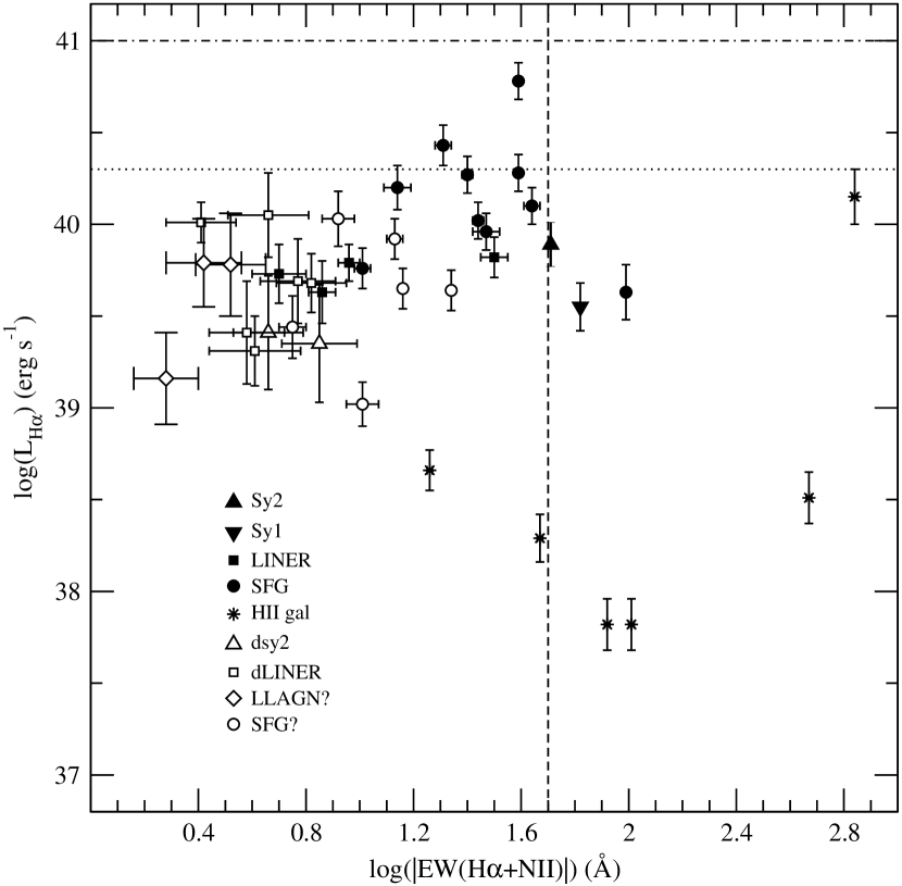
Figure 6: H$\alpha$ luminosity of the emission line galaxies (after template subtraction) as a function of the EW of the (H$\alpha+$[NII]) lines. The two horizontal lines are the mean luminosity for Markarian starburst galaxies (dash-dot) and their lower limit (dotted). The vertical (dashed) line marks the EW lower limit for actively star-forming galaxies.

In Figure 6, we compare the H$\alpha$ luminosity of the emission-line galaxies with the equivalent width of the H$\alpha+$[NII] lines. The horizontal lines indicate the mean H$\alpha$ luminosity (dot-dash) and lower limit as observed in Nuclear Starburst Galaxies (Contini, Considère & Davoust 1998). The vertical (dashed) is the dividing line between galaxies with weak and active star formation (Kennicutt & Kent 1983). It can be seen that very few SFGs in our sample qualify as a starburst or an actively star forming galaxy. In Figure 6, one can see that what seems to distinguish most LINERS and LLAGNs from SFGs are their slightly lower luminosity and distinctly smaller EW. The difference in EW, in particular, is important, since it suggests the continuum in these galaxies has a different origin (by definition, the EW is the ratio of the flux in the emission line to the continuum). This difference could be a sign of a weak AGN or of a significantly different ionizing stellar population.

Although we believe our classification is fair, we remind the reader that there is an ongoing discussion about the AGN nature of LLAGNs and LINERs (see the reviews by Lawrence 1999, and Ho 1999). Obviously, more observations will be needed before we can understand what the role of star formation and AGN activity is in these galaxies (see for example Turner et al. 2001).

In Table 3, we compare the distribution of type of activity in the present sample with that obtained in our previous analyses (Coziol et al. 1998a; Coziol, Iovino & de Carvalho 2000). For comparison, the luminous LINER and Seyfert galaxies were included in the same AGN bin. The distribution of activity type in our new sample is fully consistent with what we observed before.

3.3 Activity index

In order to quantify the level of activity in the groups, we define a new spectroscopic index for the galaxies. Since we want this index to be sensitive to the different stellar populations, and not only the ionized gas, we use the equivalent width as measured in a window centered on H$\alpha$ (Copetti, Pastoriza & Dottori 1986; Coziol 1996). The size of the window was chosen by considering the typical EWs of H$\alpha$ lines (in absorption) in the spectra of A stars, which are known to dominate the stellar population after most of the OB stars have disappeared (like in post-starburst or gas stripped galaxies; see Rose 1985; Leonardi & Rose 1996; Barbaro & Poggianti 1997), and which are responsible for the strong absorption features observed in LLAGNs (Coziol et al. 1998a). We define the activity index, EW_act, as the equivalent width measured in the rest frame of the galaxy, between 6500 Å and 6600 Å in the original spectra (i.e., without template subtraction). Defined in this way the activity index covers all the possible active states of a galaxy: active (star formation and/or AGN), decreasing star formation (post-starburst or gas stripping) and quiescent (intermediate and old stellar populations). This way of defining the activity index has the advantage that it can be easily measured in all the galaxies. The value of the activity index as measured in each galaxy in our sample is given in the last column of Table 2. The uncertainty in this value is of the order of $\pm 0.2$Å. It was estimated using the mean of the EW of all the structures (real or spurious) encountered in the continuum around the window in the four template galaxies. Note that, because of their redshifts, the O₂ atmospheric band, at 6870 Å, fell right within the window of the galaxies in HCG 8, preventing us to measure an EW_act.

In order to increase our sample of galaxies in CGs, we have measured the activity index in those galaxies that were observed in our first spectroscopical analysis of HCGs (Coziol et al. 1998a). Only four galaxies from this previous article were duplications in the present study: HCG 40a, b, e and HCG 88b. The activity indices found for these galaxies based on the 4m spectra are 0.9, 3.6, -3.0 and -5.0 Å respectively. This compares very well with the activity indices measured in our new spectra: 1.0, 3.1, -3.2 and -6.1 Å respectively.

Not considering two groups that we re-observed in the present study, and five groups where only one galaxy of each group was observed, we can add 10 CGs to our sample. The results are presented in Table 4, together with the morphological type and activity classification for each galaxy.

4 Analysis

4.1 Utility and robustness of the activity index

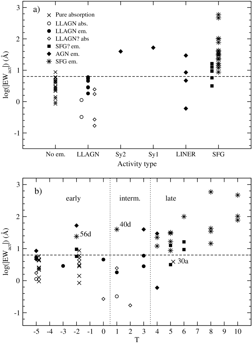
Figure 7: Value of the activity index in galaxies with different activity types (a) and morphological types (b). The horizontal dashed line separates SFGs from quiescent and LLAGNs. Using different symbols we also distinguish between absorption (EW${}_{act}>0$) and emission (EW${}_{act}<0$). The vertical (dotted) lines separate the morphology axis in three categories: early, intermediate and late-type.

Ideally, by using the mean of the activity index we should be able to discriminate between active and non-active CGs. With active CGs we mean those groups which harbor star forming galaxies and/or AGNs. To verify this, we compare, in Figure 7a, the activity index as measured in galaxies with different activity types. Since the range of the index is large, we take the logarithm and discriminate between absorption (EW${}_{act}>0$) and emission (EW${}_{act}<0$) using different symbols. In general, SFGs and luminous AGNs (Sy1, Sy2 and LINER) have EW${}_{act}<-6$ (or $\log|{\rm EW}_{act}|)>0.8$). This property allows us to separate them from quiescent galaxies and LLAGNs. We therefore adopt a mean of EW${}_{act}<-6$ to separate active from inactive groups. Note that for a mean EW${}_{act}>-6$, a negative mean index would indicate some activity, but at a significantly lower level than for active groups.

In Coziol et al. (1998a), the type of activity presented by the different galaxies was found to be correlated with their morphology. To verify if this phenomenon is also observed in the present sample, we compare the activity index with the morphological type of the galaxies in Figure 7b. In general, we find the SFGs in late-type (T $>3$) galaxies and the quiescent galaxies in early-type (T $<1$). The exceptions are HCG 56d (S0) and 40d (SBa) for the SFGs and HCG 30a (SBc) for the quiescent galaxies. We also note that AGNs and LLAGNs are usually found in intermediate and early type galaxies.

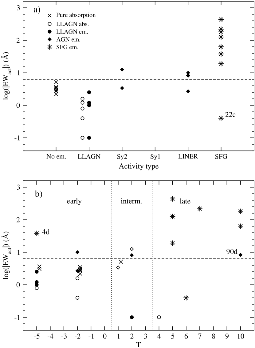
Figure 8: Value of the activity index as a function of activity types (a) and morphology (b) for the galaxies in the additional sample. The meaning of the symbols is the same as in Figure 7.

In Figure 8, we repeat our analysis for the galaxies in the complementary sample studied by Coziol et al. (1998). We distinguish the same trends as observed in our new sample. This result suggests that the activity index is independent of the type of telescope and reduction aperture used. This is most readily attributed to the compact nature of the light and ionized gas distribution in these galaxies (see our comment in Section 3.1).

4.2 Definition of evolutionary levels for CGs

As noted previously in Coziol et al. (1998a), the relation between morphology and activity as found in CGs is not specific to these systems, but is general to all galaxies independent of their environment (see e.g., Kennicutt 1992). Taken as a group, however, it was shown in the same study that the morphology-activity relation was correlated with the density of the groups. This suggests that we should combine the mean activity index with the mean morphological type of galaxies in a CG in order to quantify their level of evolution. If activity is a consequence of galaxy interactions, and if interactions lead to the formation of early–type systems, we would thus expect ”evolved” groups to be inactive and rich in early-type galaxies, whereas ”unevolved” groups would be active and rich in late-type galaxies. Another possibility is for groups to be unusually active (or inactive) considering the morphologies of their members. In the interaction scenario, such unusually active groups may constitute a genuine intermediate evolutionary level.

The mean morphological types and mean activity indices of the 27 CGs in our joined samples are reported in Table 5 ( columns 10 and 11, respectively). Note that since only one member galaxy was observed for HCG 31 this group was omitted from the rest of our analysis. In this table we have also collected other useful information on the groups as found in the literature: the systemic redshifts (column 2), as listed by Hickson in CatalogVII/213 (at the CDS); a flag indicating diffuse X ray emission (column 3), as determined by Ponman et al. (1996); the number of galaxies for which we have a spectral classification (N_S; column 4); the number of real members (N_H; column 5), as determined by Hickson (1982); the number of possible members (N_R; column 6), as determined by Ribeiro et al. (1998); the de-projected velocity dispersions (column 7), projected radii (column 8) and adopted masses (column 9) for the groups, as listed by Hickson.

4.3 Effect of incompleteness on our analysis

As mentioned in Section 2, our information on the activity of the groups is not complete due to observational constraints. To establish how this incompleteness might affect our analysis, we have assigned an activity type to the missing galaxies based on the trends between morphology and activity observed in Figure 7 and 8 and used this prediction to estimate the changes their incorporation could induce on the mean activity index and mean morphology in each group. In Table 6, we list the 16 groups for which the activity information is incomplete, identifying the missing galaxies and their morphology. In column 4 we report the observed mean activity index and in column 5 we note the change expected: a $+$ sign indicates a decrease in activity, a $-$ sign indicates an increase in activity, and a $0$ indicates no variation. It can be seen that including the missing galaxies would either have no impact or reinforce our analysis. The last two columns list both the actual mean morphological type as well as its value after taking into account the missing galaxies. Once again, only marginal changes are see. This test suggests that our present analysis is not compromised by the incompleteness of our sample.

4.4 Evolutionary sequence and spatial configuration of CGs

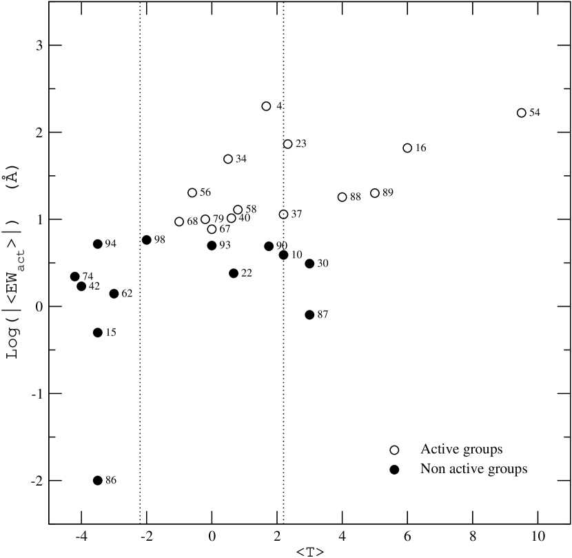
Figure 9: Mean activity index as a function of mean morphology. The CGs are identified by their HCG number. The vertical dot lines separates the groups according to the three main spatial (projected) configurations. The evolution of groups increases in the sense A$\Rightarrow$B$\Rightarrow$C

In Figure 9, we compare the mean level of activity with the mean morphological type of the galaxies in 27 HCGs. The symbols distinguish between active ($\log|{\rm EW}_{act}|)>0.8$) and inactive groups. Our sample of CGs clearly spans an evolutionary sequence. We see evolved CGs, which are inactive and dominated by elliptical galaxies, slightly less evolved groups, which look unusually active considering the early-type morphologies of their members, and non-evolved groups, which are active and dominated by late-type spirals and irregular galaxies.

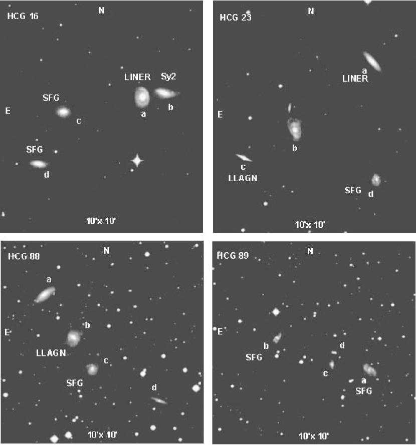
Figure 10: Type A prototypes: HCG 16, 23, 88 and 89. The letters identifying individual group members follow the notation given by Hickson (1982). The activity types from Table 2 are indicated next to their respective galaxy. The angular size of each frame is indicated along the bottom.

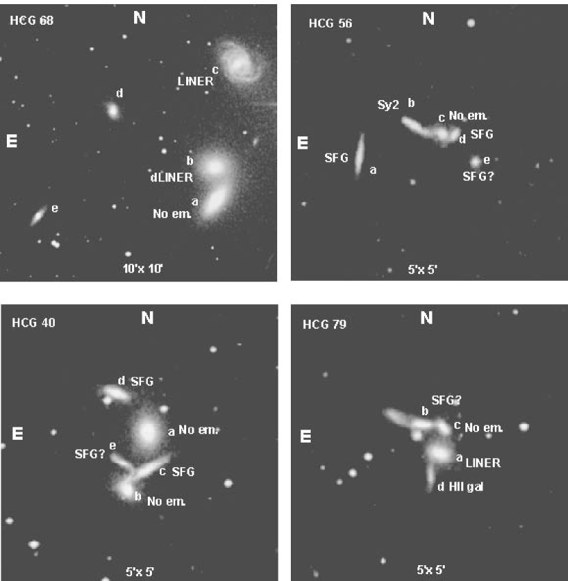
Figure 11: Type B prototypes: HCG 40, 56, 68 and 79. Same specifications as in Fig. 10.

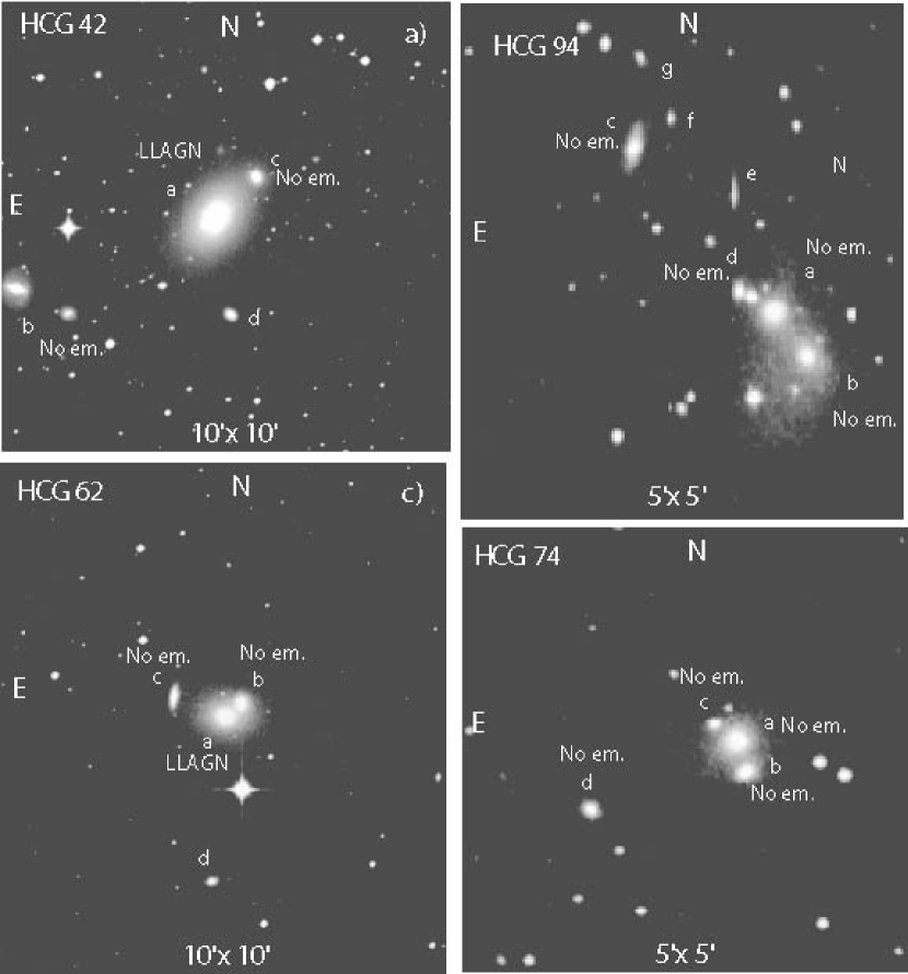
Figure 12: Type C prototypes, where one giant elliptical dominates the group: HCG 42, 62, 74 and 94. Same specifications as in Fig. 10.

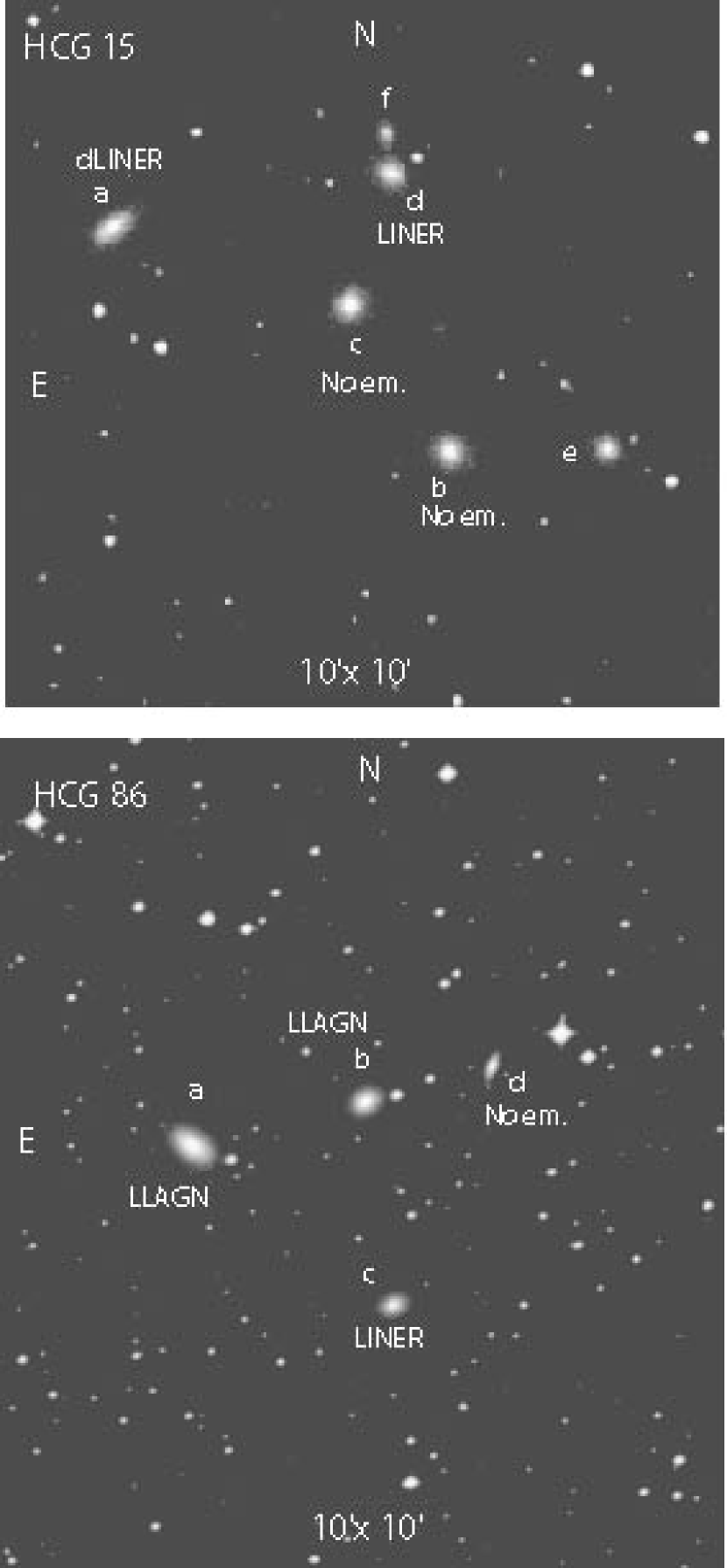
Figure 13: Type C prototypes, which are dominated by several elliptical galaxies: HCG 15 and 86. Same specifications as in Fig. 10.

At this point of our analysis, it is instructive to inspect the spatial (projected) configurations of the groups. Indeed, we find that groups that share the same level of evolution also share the same configuration. We identify three main configuration types. Type A CGs are dominated by late-type spirals and all show a loose configuration. The mean activity index for this type is high. The prototypes are HCG 16, 23, 88 and 89 and are shown in Figure 10. The two groups HCG 30 and 87 may also be classified as Type A, based on their spatial configuration, even though they are inactive. Type B consists of galaxies in apparent close contact, suggesting ongoing mergers. The prototypes are HCG 40, 56, 68 and 79 (Figure 11). A similar configuration is found for HCG 34, 37 and 67. These are all unusually active groups, considering the morphologies of their members. The three groups HCG 22, 90 and 98 may also be classified as Type B, even though they are inactive. Finally, Type C is formed by CGs that are dominated by elliptical galaxies and are inactive. The configuration is loose and the groups are either dominated by one giant elliptical, like in HCG 42, 62, 74 and 94 (Figure 12), or by more than one elliptical galaxy, like in HCG 15 and 86 (Figure 13).

Although the three CGs HCG 10, 58 and 93 seem to share the same level of evolution as groups in Type B, their spatial configurations are more similar to groups in Type A, and defy, consequently any classification.

The group HCG 54, also seems somewhat special. This group, which is remarkably active, shows the same merging configuration as CGs of Type B, but with the important difference that it is formed by irregular galaxies. The diagnostic diagram, Figure 3, suggests that the galaxies in this group are low-mass, low-metallicity HII galaxies. This is in contrast with the other CGs in our sample, which are usually formed by massive and probably metal rich galaxies (as judged from their positions in the diagnostic diagram). It is not certain, therefore, that HCG 54 describes the same phenomenon as the other groups.

Finally, according to Ribeiro et al. (1998), HCG 4 was misclassified as a CG. They showed that galaxies HCG 4e and HCG 4c weren’t group members. Eliminating them causes HCG 4 to fail the definition for a compact group according to Hickson.

Table 7 summarizes our classification for all the groups in our sample (with the exception of HCG 4). In this table, we also list the mean characteristics associated with the different Types. In columns 2 and 3, a colon following the number identifies groups with deviant or marginally deviant dynamical characteristics (for example, HCG 34 and 37 have significantly higher velocity dispersions than the other groups belonging to Type B.

Not considering the exceptions, the CGs in the different main configuration are clearly separated in Figure 9. HCGs with a mean T$>2.2$ are all Type A systems. Those with a mean T$<-2.2$ are all of Type C. Transition groups are classified as Type B. In terms of evolution, we may distinguish a continuous sequence, which goes in the sense A$\Rightarrow$B$\Rightarrow$C, where A is less evolved than C. We emphasize that in terms of spatial configuration alone, such an evolutionary sequence is not obvious (considering also the exceptions) and one needs a second parameter, such as the activity index introduced in this paper, for it to become noticeable. This may explain why the different configuration types where not recognized before.

Using a one-way ANOVA test, we confirm the differences observed between the characteristics of Types A, B and C, as shown in Table 7, at a 95% confidence level. In Table 8, we show the results of Tukey’s multiple test, that allows to identify the source of the variance. This table reports the P values for the difference between each pair of mean values. If the null hypothesis is true (all the values are sampled from populations with the same mean), then there is only a 5% chance that any one or more comparisons will have a P value less than 0.05. These tests confirm the different evolutionary level of the three types defined in this work.

4.5 The relation between galaxy activity and the dynamics of CGs

According to the conventional scenario for the fate of CGs, also referred to as the fast merger model (Mendes de Oliveira & Hickson 1994; Gómez-Flechoso & Domínguez-Tenreiro 2001), young forming groups are expected to start out with high velocity dispersions and large radii, which would rapidly decrease as the galaxies merge to form one giant elliptical (this is illustrated by the model CG2 in Figure 1 of Gómez-Flechoso & Domínguez-Tenreiro 2001). Assuming the groups form from spiral galaxies that originated in the field, we would thus expect young groups to be rich in late-type galaxies and to become gradually richer in early-type galaxies before their final merging phase. In terms of activity, we would also expect the level of star formation and AGN to be high at the beginning of the sequence and to decrease gradually, maybe with a change from star formation to AGN, in the final merger phase.

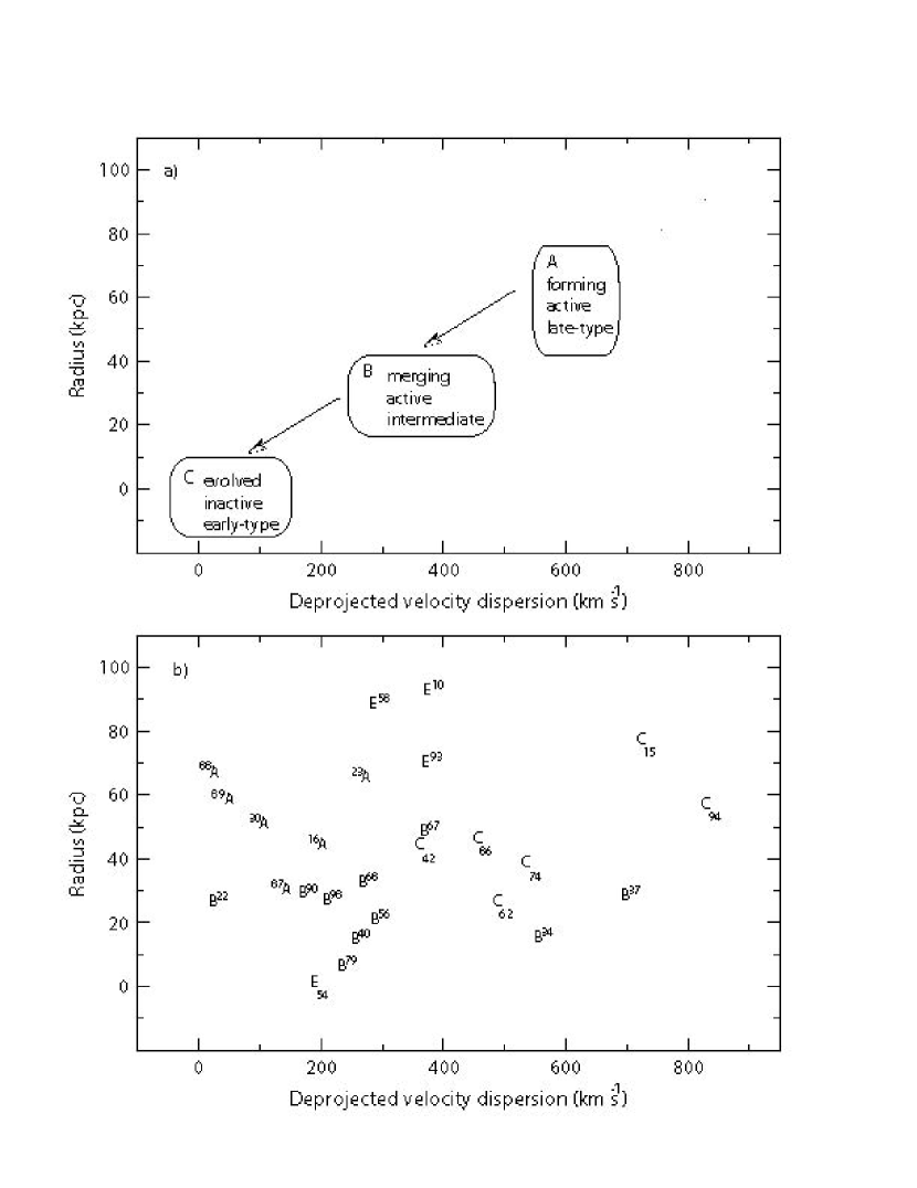
Figure 14: a) Illustration of the expected evolutionary pattern, according to the conventional fast merger model for CGs, in a diagram of radius versus velocity dispersion; b) actual positions occupied by the 26 CGs (excluding HCG 4) in our sample. The CGs are identified by their HCG number; the letters correspond to the configuration types. The E means an exception (no classification is possible).

According to the conventional fast merger model for CGs, we would thus expect to see an evolutionary sequence that would trace a very specific pattern in a graph mapping the radius as a function of the velocity dispersion. The expected pattern is sketched in Figure 14a. The actual observed positions are shown in Figure 14b. One can immediately see that the expected pattern is not reflected by the observations: CGs in Type A, which are less evolved, should have large radii and high velocity dispersions, whereas CGs in Type C, which are more evolved, should have small radii and low velocity dispersions. Contrary to expectation, Type C CGs have radii comparable to those of Type A and much higher velocity dispersions (see Table 7).

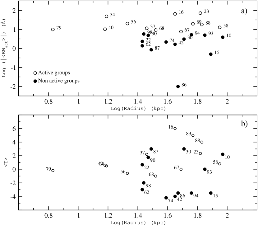
Figure 15: a) mean activity index as a function of radius. b) mean morphological type as a function of radius.

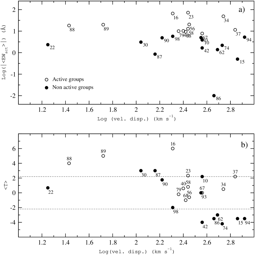
Figure 16: a) mean activity index as a function of radius. b) mean morphological type as a function of radius. The two dotted lines separates the group with different configuration types and levels of evolution (see Figure 9).

In Figure 15 we compare the mean activity index and morphology with the radius of the groups (HCG 54 was omitted). We find no relation between activity or morphology and the radius of the group. The mean activity index and morphology are compared with the velocity dispersion in Figure 16. We distinguish no relation between the activity and the velocity dispersion. However, we see a clear trend for the groups dominated by early-type galaxies to have high velocity dispersions. In terms of evolution, we see the velocity dispersion increasing from Type A to C (see also Tables 7 and 8), which indicates that the most evolved groups have the highest velocity dispersions.

The trend we observe in our sample between evolution and velocity dispersion, seems to stem from the strong correlation between morphology and velocity dispersion previously discovered by Hickson, Kindl & Huchra (1988). Our observations support their claim that the general relation between morphology and velocity dispersion encountered in CGs is an evolutionary phenomenon linked to the environment (for other evidence in favor of this interpretation see Shaker et al. 1998 and Focardi & Kelm 2002).

5 Discussion

The trends we observe in our sample are, at best, only partially consistent with the conventional fast merger model for CGs. We do distinguish what could be young forming groups (Type A) and more evolved merging groups (Type B). However, the velocity dispersions and radii of these systems are contrary to what is expected. In a sense, this negative result is somewhat discomforting, because it suggests that the dynamical evolution of galaxies in CGs is more complex than previously believed. However, this result doesn’t have to be too surprising, since this is what one expects if CGs are in reality part of larger scale structures (Rose 1977; West 1989; White 1990; Diaferio, Geller & Ramella 1994; Governato, Tozzi & Cavaliere 1996).

Assuming the formation and evolution processes of CGs are related to larger scale structures, we may have found a new clue how to explain their behavior by relating the evolutionary level of a group to its velocity dispersion. Indeed, in dynamical terms, the velocity dispersion is generally seen to increase with the total mass of the system (Heisler, Tremaine & Bahcall 1985; Perea, del Olmo & Moles 1990). By applying this observation to CGs, we may thus conclude that their level of evolution increases with their mass, or more properly, with the mass of the structure with which they are associated or where they are embedded in.

The above interpretation is supported by the three following independent observations. First, we note in Table 7 that the mean masses of the groups, as defined by Hickson (see Tables 4 and 5), does increase from types A to C. This is confirmed by a one-way ANOVA test at a 95% confidence level. In Table 8, the results of Tukey’s multiple test confirm that groups in Type C are more massive than those in Type A and B. Second, we note that the number of galaxies in structures associated with CGs generally increases with the velocity dispersion. Looking at the number of galaxies encountered by Ribeiro et al. (1998) in Table 4 and 5, we see that the structures associated with groups of Type A contain between 6 and 8 galaxies, whereas those associated with groups in Type C contain between 9 and 18 galaxies (the only exception being HCG 22). The third observation is the detection of diffuse X-ray envelopes. Naturally, one expects these envelopes to be more common or easily detected in massive systems. Using the data in Tables 4 and 5, we see that only one non–evolved group with low velocity dispersion (lower than 300 km s^-1) has an X-ray envelope. This is HCG 16 (Type A), which is unusually active (see Ribeiro et al. 1996). Another small velocity dispersion group with an X-ray envelope is the relatively evolved group HCG 58. But, this group may be considered unusually active as well, since it contains the only Sy1 in our sample. All the other X-ray envelopes are detected primarily in Type C, HCG 15, 42, 62, 86, 90, and Type B groups, HCG 37, 67, 68. With the exception of HCG 90, all these groups have velocity dispersions higher than 300 km s^-1.

Assuming that the velocity dispersion increases with the mass of the structure, a ready interpretation of our observations is that CGs associated with massive structures are more evolved. Theoretically, it is easy to find arguments in favor of this interpretation. For example, if we assume that a large number of interactions accelerates the evolution of galaxies, then we would naturally expect galaxies in more massive and rich systems to be more evolved. However, tidal interactions become less effective as collision velocities increase, which then seems in contradiction with what we observe. Alternatively, if the formation of CGs follows the formation of large scale structures then, under certain conditions, we would expect high-density structures to collapse before low density ones, forming primordially massive structures, and CGs associated with such structures to be naturally older.

Our observations are consistent with the formation of structures as predicted by the CDM model (or $\Lambda$CDM), assuming the formation of galaxies is a biased process (Davis et al. 1985; Benson et al. 2001), that is galaxies developing first in high-density structures. In terms of evolution, biased galaxy formation would naturally lead to more massive systems being more evolved (see figure one in Benson et al. 2001). If one follows the CDM model evolution over time, galaxies are seen to form first in the high-density structures, then structures are seen to get richer and more complex through mergers of smaller systems. As part of the structure formation process, the evolution of small scale entities, like CGs, must consequently be more complex than predicted by the conventional fast merger model. This is because the galaxies in these groups are possibly influenced not only by the other galaxy members, but also by the neighboring structures (see Einasto et al. 2003; Ragone et al. 2004).

As part of the structure formation process, the fate of CGs may also be different than the one predicted by the conventional fast merger model. Since structures continuously merge to form larger ones, the first groups to form (Type C), being in denser environments, would already have had time to merge with other similarly evolved groups. The most evolved groups would thus be expected today to form part of larger structures where they would be in dynamical equilibrium.

As for the groups that seem to have formed more recently (Type A), or those that formed in the recent past (Type B), the galaxies in these groups obviously have not had enough time to merge. Being found in less massive environments, it is not clear whether they will experience a complete merger of their components or whether they will find other groups with which they can merge to form larger structures (and reach equilibrium before completing the merger of their members). Such a scenario may explain some of the exceptions to the trends found in our sample, like HCG 54 (and may be HCG 31) as an example of a group in a low density environment that is completing a merger, or HCG 10, 58 and 93, as examples of different groups merging together to form a larger structure.

Finally, it is important to note that we can possibly distinguish between the two hypotheses suggested to explain our observations by examining CGs at higher redshifts. In particular, if the structure formation hypothesis is correct, one would thus expect to find CGs at higher redshift to be associated with more massive structures than those at lower redshift.

6 Summary and conclusions

We have defined a new spectroscopic index that allows us to quantify the level of activity (AGN and star formation) in galaxies. By taking the mean of this index in a CG and combining it with the mean morphological type of the galaxies it proves possible to quantify the evolutionary state of these systems.

Applying our method to a sample of 27 CGs from Hickson’s catalog, we have found an evolutionary sequence, which is correlated with the projected spatial configuration of the groups. Mapping the position of CGs with different levels of evolution and group morphology in a diagram of radius versus velocity dispersion, we did not observe the pattern predicted by the conventional fast merger model. Contrary to expectation, we found that the level of evolution of CGs increases with velocity dispersion. This trend was further shown to be possibly connected to the masses of the CGs or to the structures in which they are embedded. Assuming that the velocity dispersion increases with the mass, the trend we observe would thus imply that the most evolved groups are found within the most massive structures.

We propose two different hypotheses to explain our results. The first assumes that the evolution of galaxies accelerates with the number of interactions in massive structures. The other assumes that the formation of CGs follows the formation of the large scale structure, and that massive structures develop before less massive ones. Our observations are consistent with the formation of structures as predicted by the CDM model (or $\Lambda$CDM), assuming the formation of galaxies is a biased process: galaxies developing first in high-density structures.

Table 1: Log of the observations and main characteristics of the targets

obs.	HCG	$\alpha$	$\delta$	vr	T	Morph.	exp.	Airmass
date		(2000)	(2000)	(km s-1)			($\times 900s$)
(1)	(2)	(3)	(4)	(5)	(6)	(7)	(8)	(9)
16/10	+08a	$\phantom{0}0$ $49$ $34.26$	+$23$ $34$ $40.14$	$16014$	$-5$	E5	3	1.0
16/10	+8b	$\phantom{0}0$ $49$ $35.29$	+$23$ $35$ $28.32$	$15966$	$-2$	S0	3	1.2
16/10	+8c	$\phantom{0}0$ $49$ $35.90$	+$23$ $35$ $02.01$	$17087$	$-2$	S0	3	1.2
16/10	+08d	$\phantom{0}0$ $49$ $36.77$	+$23$ $34$ $22.80$	$16341$	$-2$	S0	3	1.0
17/10	10a	$\phantom{0}1$ $26$ $21.43$	+$34$ $42$ $07.51$	$\phantom{0}5148$	+$3$	SBb	3	1.0
17/10	10b	$\phantom{0}1$ $25$ $40.33$	+$34$ $42$ $46.39$	$\phantom{0}4862$	$-5$	E1	3	1.1
20/10	10c	$\phantom{0}1$ $26$ $18.81$	+$34$ $45$ $14.38$	$\phantom{0}4660$	+$5$	Sc	3	1.0
20/10	10d	$\phantom{0}1$ $26$ $30.84$	+$34$ $40$ $30.46$	$\phantom{0}4620$	+$6$	Scd	3	1.1
18/10	15a	$\phantom{0}2$ $07$ $53.00$	+$02$ $10$ $03.31$	$\phantom{0}6967$	+$1$	Sa	3	1.2
19/10	15b	$\phantom{0}2$ $07$ $34.09$	+$02$ $06$ $54.73$	$\phantom{0}7117$	$-5$	E0	3	1.1
19/10	15c	$\phantom{0}2$ $07$ $39.75$	+$02$ $08$ $59.02$	$\phantom{0}7222$	$-5$	E0	3	1.1
19/10	15d	$\phantom{0}2$ $07$ $37.49$	+$02$ $10$ $50.80$	$\phantom{0}6244$	$-5$	E2	3	1.2
19/10	30a	$\phantom{0}4$ $36$ $18.57$	$-02$ $49$ $52.67$	$\phantom{0}4697$	+$5$	SBc	3	1.2
19/10	30b	$\phantom{0}4$ $36$ $30.27$	$-02$ $51$ $59.66$	$\phantom{0}4625$	+$1$	Sa	3	1.2
20/10	31a	$\phantom{0}5$ $01$ $38.74$	$-04$ $15$ $34.11$	$\phantom{0}4042$	+$8$	Sdm	4	1.2
17/10	34a	$\phantom{0}5$ $21$ $45.93$	+$06$ $41$ $19.73$	$\phantom{0}8997$	$-5$	E2	3	1.1
17/10	34c	$\phantom{0}5$ $21$ $48.96$	+$06$ $40$ $54.71$	$\phantom{0}9392$	+$6$	SBd	1	1.2
08/04	37a	$\phantom{0}9$ $13$ $39.44$	+$29$ $59$ $32.61$	$\phantom{0}6745$	$-3$	E7	3	1.0
08/04	+37b	$\phantom{0}9$ $13$ $32.60$	+$29$ $59$ $59.04$	$\phantom{0}6741$	+$4$	Sbc	6	1.0
08/04	+37c	$\phantom{0}9$ $13$ $37.22$	+$29$ $59$ $58.22$	$\phantom{0}7357$	+$0$	S0a	6	1.0
08/04	37d	$\phantom{0}9$ $13$ $33.84$	+$30$ $00$ $51.78$	$\phantom{0}6207$	+$8$	SBdm	3	1.1
10/04	40a	$\phantom{0}9$ $38$ $53.52$	$-04$ $50$ $56.53$	$\phantom{0}6628$	$-5$	E3	3	1.2
10/04	40b	$\phantom{0}9$ $38$ $55.04$	$-04$ $51$ $57.90$	$\phantom{0}6842$	$-2$	S0	3	1.2
10/04	40c	$\phantom{0}9$ $38$ $53.20$	$-04$ $51$ $33.72$	$\phantom{0}6890$	+$4$	Sbc	3	1.3
10/04	40d	$\phantom{0}9$ $38$ $55.77$	$-04$ $50$ $14.53$	$\phantom{0}6492$	+$1$	SBa	3	1.3
10/04	40e	$\phantom{0}9$ $38$ $55.45$	$-04$ $51$ $27.91$	$\phantom{0}6625$	+$5$	Sc	3	1.2
09/04	+54a	$11$ $29$ $15.17$	+$20$ $35$ $00.73$	$\phantom{0}1397$	+$8$	Sdm	4	1.0
09/04	+54b	$11$ $29$ $14.05$	+$20$ $34$ $53.24$	$\phantom{0}1412$	+$10$	Im	4	1.0
09/04	54c	$11$ $29$ $16.26$	+$20$ $35$ $11.12$	$\phantom{0}1420$	+$10$	Im	3	1.0
09/04	54d	$11$ $29$ $16.50$	+$20$ $35$ $18.82$	$\phantom{0}1670$	+$10$	Im	3	1.1
08/04	+56a	$11$ $32$ $46.64$	+$52$ $56$ $27.03$	$\phantom{0}8245$	+$5$	Sc	3	1.5
08/04	+56b	$11$ $32$ $40.45$	+$52$ $57$ $01.59$	$\phantom{0}7919$	$-2$	SB0	5	1.1
08/04	56c	$11$ $32$ $36.69$	+$52$ $56$ $51.03$	$\phantom{0}8110$	$-2$	S0	3	1.1
08/04	56d	$11$ $32$ $35.29$	+$52$ $56$ $49.84$	$\phantom{0}8346$	$-2$	S0	3	1.2
08/04	56e	$11$ $32$ $32.73$	+$52$ $56$ $20.96$	$\phantom{0}7924$	$-2$	S0	3	1.3
10/04	58a	$11$ $42$ $11.06$	+$10$ $16$ $39.62$	$\phantom{0}6138$	+$3$	Sb	3	1.1
10/04	58b	$11$ $42$ $23.56$	+$10$ $15$ $51.05$	$\phantom{0}6503$	+$2$	SBab	3	1.1
10/04	58c	$11$ $41$ $53.15$	+$10$ $18$ $14.63$	$\phantom{0}6103$	+$0$	SB0a	3	1.2
10/04	58d	$11$ $42$ $05.89$	+$10$ $21$ $03.06$	$\phantom{0}6270$	$-5$	E1	3	1.2
10/04	58e	$11$ $42$ $04.82$	+$10$ $23$ $01.86$	$\phantom{0}6052$	+$4$	Sbc	3	1.4
09/04	68a	$13$ $53$ $26.53$	+$40$ $16$ $58.35$	$\phantom{0}2162$	$-2$	S0	3	1.0
09/04	68b	$13$ $53$ $26.62$	+$40$ $18$ $08.65$	$\phantom{0}2635$	$-5$	E2	3	1.0
09/04	68c	$13$ $53$ $21.69$	+$40$ $21$ $47.68$	$\phantom{0}2313$	+$4$	SBbc	4	1.1
08/04	74a	$15$ $19$ $24.91$	+$20$ $53$ $44.17$	$12255$	$-5$	E1	3	1.1
09/04	74b	$15$ $19$ $24.38$	+$20$ $53$ $23.44$	$12110$	$-5$	E3	3	1.1
09/04	74c	$15$ $19$ $26.18$	+$20$ $53$ $56.44$	$12266$	$-2$	S0	3	1.1
09/04	74d	$15$ $19$ $32.02$	+$20$ $52$ $57.47$	$11681$	$-5$	E2	3	1.2
07/04	79a	$15$ $59$ $11.41$	+$20$ $45$ $14.86$	$\phantom{0}4292$	$-5$	E0	3	1.0
07/04	79b	$15$ $59$ $12.61$	+$20$ $45$ $47.14$	$\phantom{0}4446$	$-2$	S0	3	1.0
07/04	79c	$15$ $59$ $10.95$	+$20$ $45$ $41.43$	$\phantom{0}4146$	$-2$	S0	2	1.0
10/04	79d	$15$ $59$ $12.01$	+$20$ $44$ $47.20$	$\phantom{0}4503$	+$8$	Sdm	3	1.1
17/10	88b	$20$ $52$ $29.69$	$-05$ $44$ $47.61$	$\phantom{0}6010$	+$3$	SBb	4	1.2
17/10	88c	$20$ $52$ $25.94$	$-05$ $46$ $20.12$	$\phantom{0}6083$	+$5$	Sc	2	1.3
16/10	89a	$21$ $20$ $01.03$	$-03$ $55$ $20.26$	$\phantom{0}8850$	+$5$	Sc	3	1.2
16/10	89b	$21$ $20$ $19.21$	$-03$ $53$ $46.81$	$\phantom{0}8985$	+$5$	SBc	3	1.5
17/10	93a	$23$ $15$ $15.98$	+$18$ $57$ $41.36$	$\phantom{0}5140$	$-5$	E1	3	1.0
17/10	93b	$23$ $15$ $17.17$	+$19$ $02$ $29.77$	$\phantom{0}4672$	+$6$	SBd	3	1.0
17/10	93c	$23$ $15$ $03.59$	+$18$ $58$ $23.28$	$\phantom{0}5132$	+$1$	SBa	3	1.1
20/10	93d	$23$ $15$ $33.10$	+$19$ $02$ $52.50$	$\phantom{0}5173$	$-2$	SB0	3	1.0
18/10	+94a	$23$ $17$ $13.44$	+$18$ $42$ $28.22$	$12040$	$-5$	E1	3	1.0
18/10	+94b	$23$ $17$ $11.94$	+$18$ $42$ $03.30$	$11974$	$-5$	E3	3	1.0
18/10	+94c	$23$ $17$ $20.26$	+$18$ $44$ $03.62$	$12120$	$-2$	S0	3	1.0
20/10	94d	$23$ $17$ $15.19$	+$18$ $42$ $42.55$	$13009$	$-2$	S0	3	1.1
18/10	+98a	$23$ $54$ $10.08$	+$00$ $22$ $58.07$	$\phantom{0}7855$	$-2$	SB0	5	1.2
18/10	+98b	$23$ $54$ $12.21$	+$00$ $22$ $35.88$	$\phantom{0}7959$	$-2$	S0	5	1.2

Table 2: Observed line ratios, fluxes and Equivalent Widths

HCG	Ap.	$\log$([NII]/H$\alpha$)	$\log$([OIII]/H$\beta$)	$\log($L${}_{{\rm H}\alpha})$	EW(H$\alpha+{\rm NII}$)	Act. type	EWact
	(kpc)			(erg s-1)	(Å)		(Å)
(1)	(2)	(3)	(4)	(5)	(6)	(7)	(8)
08a	12	$\cdots$	$\cdots$	$\cdots$	$\cdots$	No em.	$\cdots$
08b	11	$\cdots$	$\cdots$	$\cdots$	$\cdots$	No em.	$\cdots$
08c	10	$\cdots$	$\cdots$	$\cdots$	$\cdots$	No em.	$\cdots$
08d	11	$\cdots$	$\cdots$	$\cdots$	$\cdots$	No em.	$\cdots$
10a	4	+$0.39\pm 0.10$	+$0.76\pm 0.17$	39.4:	$-5$	dSy2	$-2.8$
10b	3	$\cdots$	$\cdots$	$\cdots$	$\cdots$	No em.	+$2.6$
10c	3	$-0.33\pm 0.02$	$\cdots$	39.6	$-15$	SFG?	$-12.5$
10d	3	$-0.29\pm 0.03$	$\cdots$	39.0	$-10$	SFG?	$-9.4$
15a	4	$-0.01\pm 0.08$	$-0.19\pm 0.15$	40.0	$-3$	dLINER	$0.3$
15b	4	$\cdots$	$\cdots$	$\cdots$	$\cdots$	No em.	$4.4$
15c	4	$\cdots$	$\cdots$	$\cdots$	$\cdots$	No em.	$5.7$
15d	4	$-0.02\pm 0.04$	+$0.11\pm 0.06$	39.8	$-9$	LINER	$-8.6$
30a	3	$\cdots$	$\cdots$	$\cdots$	$\cdots$	No em.	$3.8$
30b	2	$\cdots$	$-0.34\pm 0.16$	$\cdots$	$\cdots$	LLAGN?	$2.4$
$+$31a	3	$-0.95\pm 0.02$	+$0.44\pm 0.02$	40.2	$-693$	HIIgal	$-592.1$
34a	5	+$0.02\pm 0.08$	$\cdots$	39.8:	$-3$	LLAGN?	$1.7$
$+$34c	6	$-0.52\pm 0.05$	$-0.02\pm 0.06$	39.6	$-97$	SFG	$-100.4$
37a	7	+$0.23\pm 0.06$	+$0.22\pm 0.22$	40.0:	$-5$	dLINER	$-2.9$
37b	13	$-0.19\pm 0.07$	+$0.10\pm 0.16$	39.7	$-5$	LINER	$-0.6$
37c	10	$-0.28\pm 0.10$	$\cdots$	39.2:	$-2$	LLAGN?	$0.3$
37d	6	$-0.57\pm 0.01$	$-0.46\pm 0.08$	40.1	$-44$	SFG	$-42.2$
40a	5	$\cdots$	$\cdots$	$\cdots$	$\cdots$	No em.	$1.0$
40b	6	$\cdots$	$\cdots$	$\cdots$	$\cdots$	No em.	$3.1$
40c	8	$-0.23\pm 0.01$	$-0.30\pm 0.09$	40.2	$-14$	SFG	$-12.0$
40d	5	$-0.28\pm 0.01$	$-0.46\pm 0.08$	40.8	$-38$	SFG	$-40.1$
40e	6	$-0.31\pm 0.01$	$\cdots$	39.4	$-6$	SFG?	$-3.2$
54a	1	$-0.90\pm 0.03$	+$0.51\pm 0.06$	38.7	$-18$	HIIgal	$-14.4$
$+$54b	1	$-1.36\pm 0.03$	+$0.68\pm 0.03$	38.5	$-471$	HIIgal	$-472.4$
$+$54c	1	$-1.12\pm 0.02$	+$0.37\pm 0.03$	37.8	$-84$	HIIgal	$-78.5$
$+$54d	1	$-1.23\pm 0.05$	+$0.57\pm 0.05$	37.8	$-102$	HIIgal	$-102.7$
56a	25	$-0.42\pm 0.01$	+$0.01\pm 0.04$	40.4	$-20$	SFG	$-16.8$
$+$56b	5	$-0.04\pm 0.01$	+$1.45\pm 0.02$	39.9	$-52$	Sy2	$-52.1$
56c	6	$\cdots$	$\cdots$	$\cdots$	$\cdots$	No em.	$1.4$
56d	11	$-0.28\pm 0.02$	$-0.10\pm 0.02$	40.3	$-25$	SFG	$-23.9$
56e	7	$-0.48\pm 0.02$	$\cdots$	39.9	$-14$	SFG?	$-9.4$
$+$58a	4	$\cdots$	$\cdots$	39.6	$-66$	Sy1.8	$-39.8$
58b	5	+$0.07\pm 0.18$	$\cdots$	39.8:	$-3$	LLAGN?	$0.2$
58c	5	+$0.10\pm 0.11$	+$0.15\pm 0.16$	39.7:	$-6$	dLINER	$-4.6$
58d	5	$\cdots$	$\cdots$	$\cdots$	$\cdots$	No em.	$2.2$
58e	5	$-0.54\pm 0.02$	$-0.49\pm 0.15$	40.0	$-28$	SFG	$-22.4$
68a	3	$\cdots$	$\cdots$	$\cdots$	$\cdots$	No em.	$0.9$
68b	2	$-0.19\pm 0.2$	+$0.14\pm 0.17$	39.4:	$-4$	dLINER	$1.1$
68c	2	$-0.06\pm 0.02$	$-0.02\pm 0.05$	39.8	$-31$	LINER	$-29.6$
74a	14	$\cdots$	$\cdots$	$\cdots$	$\cdots$	No em.	$1.3$
74b	11	$\cdots$	$\cdots$	$\cdots$	$\cdots$	No em.	$2.5$
74c	7	$\cdots$	$\cdots$	$\cdots$	$\cdots$	No em.	$2.8$
74d	9	$\cdots$	$\cdots$	$\cdots$	$\cdots$	No em.	$2.2$
79a	4	$-0.28\pm 0.05$	+$0.28\pm 0.11$	39.6	$-7$	LINER	$-4.6$
79b	5	$-0.31\pm 0.05$	$\cdots$	40.0	$-8$	SFG?	$-6.0$
79c	3	$\cdots$	$\cdots$	$\cdots$	$\cdots$	No em.	$5.0$
$+$79d	5	$-1.05\pm 0.05$	+$0.39\pm 0.04$	38.3	$-47$	HIIgal	$-34.6$
88b	3	+$0.28\pm 0.09$	+$0.51\pm 0.20$	39.4:	$-7$	dSy2	$-6.1$
88c	6	$-0.50\pm 0.01$	$-0.41\pm 0.04$	40.0	$-30$	SFG	$-29.9$
89a	5	$-0.40\pm 0.02$	$-0.37\pm 0.07$	39.8	$-10$	SFG	$-8.7$
89b	6	$-0.56\pm 0.01$	$-0.10\pm 0.04$	40.3	$-39$	SFG	$-31.3$
93a	3	+$0.13\pm 0.11$	+$0.24\pm 0.14$	39.7	$-7$	dLINER	$-5.4$
93b	2	$-0.39\pm 0.02$	$\cdots$	39.6	$-22$	SFG?	$-16.4$
93c	3	$-0.09\pm 0.10$	$-0.12\pm 0.17$	39.3	$-4$	dLINER	$-1.8$
93d	3	$\cdots$	$\cdots$	$\cdots$	$\cdots$	No em.	$3.8$
94a	6	$\cdots$	$\cdots$	$\cdots$	$\cdots$	No em.	$4.5$
94b	6	$\cdots$	$\cdots$	$\cdots$	$\cdots$	No em.	$4.3$
94c	7	$\cdots$	$\cdots$	$\cdots$	$\cdots$	No em.	$6.1$
94d	6	$\cdots$	$\cdots$	$\cdots$	$\cdots$	No em.	$6.0$
98a	5	$\cdots$	$\cdots$	$\cdots$	$\cdots$	No em.	$8.6$
98b	4	$\cdots$	$\cdots$	$\cdots$	$\cdots$	No em.	$3.0$

Table 3: Activity classification in CGs

	No em.	LLAGN	AGN	SFG
This work (65gal/19gr)	38%	19%	9%	34%
HCG (62gal/17gr)	40%	21%	18%	21%
SCG (193gal/49gr)	27%	22%	19%	32%

Table 4: Activity indices and characteristics of the additional sample

HCG	Act. Type	Morph.	T	EWact
4a	SFG	Sc	5	-127.0
4b	SFG	Sc	5	-431.8
4d	SFG	E4	-5	-38.4
16a	LINER	SBab	2	-8.2
16b	Sy2	Sab	2	-12.5
16c	SFG	Im	10	-180.2
16d	SFG	Im	10	-63.1
22a	LLAGN	E2	-5	0.8
22b	No Em.	Sa	1	5.1
22c	SFG	SBcd	6	-0.4
23a	LLAGN	Sab	2	-0.1
23c	LLAGN	S0	-2	0.4
23d	SFG	Sd	7	-219.8
42a	LLAGN	E3	-5	-1.0
42b	No Em.	SB0	-2	2.8
42c	No Em.	E2	-5	3.1
62a	LLAGN	E3	-5	-2.5
62b	No Em.	S0	-2	3.5
62c	No Em.	S0	-2	3.1
67a	No Em.	E1	-5	3.6
67b	SFG	Sc	5	-19.0
86a	LLAGN	E2	-5	1.2
86b	LLAGN	E2	-5	-1.2
86c	LINER	SB0	-2	-2.7
86d	No Em.	S0	-2	2.7
87a	LLAGN	Sbc	4	0.1
87b	LLAGN	S0	-2	1.6
90a	Sy2	Sa	1	-3.4
90b	LINER	E0	-2	-10.1
90c	No Em.	E0	-2	2.2
90d	LINER	Im	10	-8.4

Table 5: Mean activity index and morphology of CGs

HCG	z	diff. X	NS	NH	NR	vel. disp.	radius	log(Mass)	$\langle$T$\rangle$	$\langle{\rm EW}_{act}\rangle$
						(km s-1)	(kpc)	(g)
(1)	(2)	(3)	(4)	(5)	(6)	(7)	(8)	(9)	(10)	(11)
04	0.0280	?	3	$\cdots$	$\cdots$	$575$	$58$	46.45	+$1.7$	$-199$
10	0.0161	$\cdots$	4	$\cdots$	$\cdots$	363	93	46.09	+2.2	00$-4$
15	0.0228	yes	4	6	$\cdots$	724	78	46.86	$-3.5$	+00$0$
16	0.0132	yes	4	$\cdots$	0$7$	$204$	$45$	45.41	+$6.0$	0$-66$
22	0.0090	$\cdots$	3	$\cdots$	0$4$	018	$27$	43.70	+$0.7$	+00$2$
23	0.0161	$\cdots$	3	4	0$8$	$275$	$66$	45.95	+$2.3$	0$-73$
30	0.0154	$\cdots$	2	4	$\cdots$	110	51	44.96	+3.0	+00$3$
34	0.0307	$\cdots$	2	4	$\cdots$	550	15	45.90	+0.5	0$-49$
37	0.0223	yes	4	5	$\cdots$	692	29	46.25	+2.2	0$-11$
40	0.0223	$\cdots$	5	5	7	251	15	45.26	+0.6	0$-10$
42	0.0133	yes	3	4	$11$	$363$	$45$	45.83	$-4.0$	+00$2$
54	0.0049	$\cdots$	4	$\cdots$	$\cdots$	182	02	43.88	+9.5	$-167$
56	0.0270	$\cdots$	5	$\cdots$	$\cdots$	282	21	45.34	$-0.6$	0$-20$
58	0.0207	yes	5	$\cdots$	$\cdots$	275	89	45.98	+0.8	0$-13$
62	0.0137	yes	3	4	$\cdots$	$490$	$27$	45.87	$-3.0$	+00$1$
67	0.0245	yes	2	4	14	$363$	$49$	46.03	+$0.0$	+0$-8$
68	0.0080	yes	3	5	$\cdots$	263	33	45.47	$-1.0$	00$-9$
74	0.0399	$\cdots$	4	5	$\cdots$	537	39	46.32	$-4.2$	+00$2$
79	0.0145	$\cdots$	4	$\cdots$	$\cdots$	229	07	44.83	$-0.2$	0$-10$
86	0.0199	yes	4	$\cdots$	$\cdots$	$457$	$47$	46.20	$-3.5$	+00$0$
87	0.0296	$\cdots$	3	$\cdots$	0$6$	$145$	$31$	44.91	+$3.0$	+00$1$
88	0.0201	$\cdots$	2	4	6	027	68	$\cdots$	+4.0	0$-18$
89	0.0297	$\cdots$	2	4	$\cdots$	052	59	44.86	+5.0	0$-20$
90	0.0088	yes	4	$\cdots$	0$9$	$166$	$30$	45.00	+$1.8$	+0$-5$
93	0.0168	$\cdots$	4	$\cdots$	$\cdots$	355	71	46.10	+0.0	00$-5$
94	0.0417	$\cdots$	5	7	$\cdots$	832	58	46.72	$-3.5$	+00$5$
98	0.0266	$\cdots$	2	3	$\cdots$	204	28	45.35	$-2.0$	+00$6$

Table 6: Effect expected of incompleteness on our analysis

HCG	Missing gal.	Morph.	$\langle{\rm EW}_{\rm act}\rangle$	changes	$\langle$T$\rangle$	$\langle$T$\rangle_{C}$
04	c	E2	$-199$	$+$	+$1.7$	+$0.0$
15	e,f	Sa, Sbc	+00$0$	$0$	$-2.4$	$-0.1$
23	b,	Sc	0$-73$	$-$	+$2.3$	+$3.0$
30	c, d	SBc, S0	+00$3$	$0$	+$3.0$	+$2.0$
34	b, d	Sd, S0	0$-49$	$0$	+$0.5$	+$1.5$
37	e	E0	0$-11$	$+$	+$2.2$	+$1.4$
40	c	Sbc	0$-10$	$-$	$-0.2$	+$0.6$
42	d	E	+00$2$	$+$	$-4.0$	$-4.2$
62	d	E	+00$1$	$+$	$-3.0$	$-3.5$
67	c, d	Scd, S0	+0$-8$	$0$	+$0.0$	+$1.0$
68	de, e	E, S0	00$-9$	$+$	$-1.0$	$-2.0$
74	e	S0	+00$2$	$+$	$-4.2$	$-3.8$
88	a, d	Sbc, Sc	0$-18$	$-$	+$4.0$	+$4.2$
89	c, d	Scd, Sm	0$-20$	$-$	+$5.0$	+$6.2$
94	e, f, g	Sd, S0, S0	+00$5$	$+$	$-3.5$	$-1.6$
98	c	E	+00$6$	$+$	$-2.0$	$-0.8$

Table 7: Configuration Types and mean properties

Type	HCG group #		$\langle{\rm Vel.disp.}\rangle$	$\langle{\rm Radius}\rangle$	$\langle{\rm M}\rangle$	$\langle{\rm T}\rangle$	$\langle{\rm EW}\rangle$
	active	inactive	(km s-1)	(kpc)	(g)		(Å)
(1)	(2)	(3)	(4)	(5)	(6)	(7)	(8)
A	16, 23, 88, 89	30, 87	$135\pm 38$	$53\pm 6$	$45.2\pm.2$	+$3.9\pm 0.6$	$-29\pm 13$
B	37:, 34:, 40, 56, 67, 68, 79	22, 90, 98	$302\pm 61$	$25\pm 4$	$45.3\pm.2$	+$0.2\pm 0.4$	$-11\pm\phantom{0}5$
C	$\cdots$	15, 42, 62:, 86, 74, 94	$567\pm 72$	$49\pm 7$	$46.2\pm.2$	$-3.6\pm 0.2$	+$\phantom{0}2\pm\phantom{0}1$
exceptions	10, 54, 4	58, 93	$\cdots$	$\cdots$	$\cdots$	$\cdots$	$\cdots$

Table 8: Results for Tukey’s post tests

Types	$\langle{\rm Vel.disp.}\rangle$	$\langle{\rm Radius}\rangle$	$\langle{\rm M}\rangle$	$\langle{\rm T}\rangle$	$\langle{\rm EW}\rangle$
A-B	$>0.05$	$<0.01$	$>0.05$	$<0.001$	$>0.05$
A-C	$<0.001$	$>0.05$	$<0.05$	$<0.001$	$<0.05$
B-C	$<0.05$	$<0.05$	$<0.05$	$<0.001$	$>0.05$

References

- (1) Aceves, H. & Velázquez, H. 2002, RMA&A, 38, 199
- (2) Barnes, J. E. 1989, Nature, 338, 123
- (3) Barbaro, G. & Poggianti, A&A, 324, 490
- (4) Barton, E. J., De Carvalho, R. R. & Geller, M. J. 1998, AJ, 116, 1573
- (5) Benson, A. J., Frenk, C. S., Baugh, C. M., Cole, S., & Lacey, C. G. 2001, MNRAS, 327, 1041
- (6) Byrd, G. & Valtonen, M. 1990, ApJ, 350, 89
- (7) Contini, T., Considère, S. & Davoust, E. 1998, A&AS, 130, 285
- (8) Copetti, M. V. F., Pastoriza, M. G. & Dottori, H. A. 1986, A&A, 156, 111
- (9) Coziol, R. 1996, A&A, 309, 345
- (10) Coziol, R., Ribeiro, A. L. B., Capelato, H. V. & de Carvalho, R. R. 1998a, ApJ, 493, 563
- (11) Coziol, R., de Carvalho, R. R., Capelato, H. V. & Ribeiro, A. L. B. 1998b, ApJ, 506, 545
- (12) Coziol, R., Iovino, A. & de Carvalho, R. R. 2000, AJ, 120, 47
- (13) Davis, M., Efstathiou, G., Frenk, C. S. & White, S. D. M. 1985, ApJ, 292, 371
- (14) Diaferio, A., Geller, M. J. & Ramella, M. 1994, AJ, 107, 868
- (15) Einasto, M., Einasto, J., Müller, V., Heimämäki, P. & Tucker, D. L. 2003, A&A, 401, 851
- (16) Focardi, P. & Kelm, B. 2002, A&A 391, 35
- (17) Fugita, Y. 1998, ApJ, 509, 587
- (18) Garcia, A. M. 1995, A&A, 297, 56
- (19) Gómez-Flechoso & M. A., Domínguez-Tenreiro, R. 2001, ApJ, 549, 187
- (20) Governato, F., Tozzi, P. & Cavaliere, A. 1996, ApJ, 458, 18
- (21) Heisler, J., Tremaine, S. & Bahcall, J. N. 1985, ApJ, 298, 8
- (22) Henriksen, M. J. & Byrd, G. 1996, ApJ, 459, 82
- (23) Hickson, P. 1982, ApJ, 255, 382
- (24) Hickson, P. Kindl, E. & Huchra J. P. 1988, ApJ, 331, 64
- (25) Ho, L. 1999, AdSpR, 23, 813
- (26) Kennicutt, R. C. Jr. 1992, ApJS, 79, 255
- (27) Kennicutt, R. C. Jr. & Kent, S. M., 1983, AJ, 88, 1094
- (28) Lawrence, A. 1999, AdSpR, 23, 1167
- (29) Leonardi, A. J. & Rose, J. A. 1996, AJ, 111, 182
- (30) Mendes de Oliveira, C. & Hickson 1994, ApJ 427, 684
- (31) Merritt, D. 1983, ApJ, 264, 24
- (32) Merritt, D. 1984, ApJ, 276, 26
- (33) Miller, N. A. & Owen, F. N. 2002, AJ, 124, 2453
- (34) Osterbrock, D. E. 1981, ApJ, 249, 462
- (35) Perea, J., del Olmo, A. & Moles, M. 1990, A&A, 237, 319
- (36) Ponman, T. J., Bourner, P. D. J., Ebeling, H. & Böhringer 1996, MNRAS, 283, 690
- (37) Ragone, C. J., Merchán, M., Muriel, H. & Zandivarez, A. 2004, MNRAS, in press (astro-ph0402155)
- (38) Ramella, M., Diaferio, A., Geller, M. J., Huchra, J. P. 1994, AJ, 107, 1623
- (39) Ribeiro, A. L. B., De Carvalho, R. R., Coziol, R., Capelato, H. V. & Zepf, S. E. 1996, ApJ, 463, L5
- (40) Ribeiro, A. L. B., De Carvalho, R. R., Capelato, H. V. & Zepf, S. E. 1998, ApJ, 497, 72
- (41) Rood, H. J., Struble, M. F. 1994, PASP, 106, 413
- (42) Rose, J. A. 1985, AJ, 90, 1927
- (43) Rose, J. A. 1977, ApJ, 211, 311
- (44) Shaker, A. A., Longo, G., Merluzzi, P. 1998, AN, 319, 167
- (45) Severgnini, P., Garilli, B., Saracco, P. & Chincarini, G. 1999, A&AS, 137, 495
- (46) Turner, M. J. L., Reeves, J. N., Ponman, T. J. et al. 2001, A&A, 365, 110
- (47) Veilleux, S. & Osterbrock, D. E. 1987, ApJS, 63, 295
- (48) White, S. D. M. in Dynamics and Interactions of Galaxies, p. 380
- (49) West, M. J. 1989, ApJ, 344, 535