Superposition of blackbodies and the dipole anisotropy:
A possibility to calibrate CMB experiments

The CMB angular temperature fluctuations observed by Cobe and Wmap enable us to place a lower limit on the spectral distortions of the CMB at any angular scale. These distortions are connected with the simple fact, that the superposition of blackbodies with different temperatures in general is not a blackbody. We show, that in the limit of small temperature fluctuations, the superposition of blackbodies leads to a y-type spectral distortion. It is known, that the CMB dipole induces a y-type spectral distortion with quadrupole and monopole angular distribution leading to a corresponding whole sky y-parameter of $y_{\rm d}=2.6\cdot 10^{-7}$. We show here that taking the difference of the CMB signal in the direction of the maximum and minimum of the CMB dipole due to the superposition of two blackbodies leads to a spectral distortion with $y_{\rm opt}=12\,y_{\rm d}=3.1\cdot 10^{-6}$. The amplitude of this distortion can be calculated to the same precision as the CMB dipole, i.e. $0.3\%$ today. Therefore it may be used as a source with brightness of several or tens of $\mu\,$K to cross calibrate and calibrate different frequency channels of CMB surveys with precision of a few tens or hundreds of nK. Furthermore, we show in this work that primordial anisotropies for multipoles $2\leq l\leq 1000$ also lead to spectral distortions but with much smaller y-parameter, i.e. $y\sim 10^{-11}-10^{-9}$.

1 Introduction

The Wmap spacecraft measured the amplitude of the angular fluctuations of the cosmic microwave background (CMB) temperature with extremely high precision on a very broad range of angular scales, from $12^{\prime}$ up to the whole sky. These temperature anisotropies and the existence of the acoustic peaks were predicted already long ago (Peebles & Yu, 1970; Sunyaev & Zeldovich, 1970a), but only now after Boomerang, Maxima, Archeops, Wmap and many ground based experiments like Cbi, Acbar, Vsa, etc. we know their precise characteristic angular scales and amplitudes. With no doubt, only tiny fluctuations of the radiation temperature field have been observed, but nowadays with a precision to better than 1% down to degree angular scales.

It is commonly assumed that the spectrum in one direction of the sky is planckian and that only the temperature changes from point to point. This follows from the nature of the main effects leading to the appearance of these fluctuations, i.e. the Sachs-Wolfe-effect (Sachs & Wolfe, 1967) and the Doppler effect due to Thomson scattering off moving electrons (Sunyaev & Zeldovich, 1970a) at redshift $\sim 1100$. However, as will be demonstrated below, there are spectral distortions in second order of $\Delta T/T$. These distortions are inevitable when the CMB is observed with finite angular resolution or when regions on the sky containing blackbodies with different temperatures are compared with each other.

The CMB missions mentioned above have shown that there are fluctuations of the radiation temperature on the level of $\Delta T\sim\mu$K$-$mK over a broad range of angular scales. One may distinguish two basic observational strategies: (i) absolute measurements, where the beam flux in some direction on the sky is compared to an internal calibrator (Cobe/Firas) and (ii) differential measurements, where the beam flux in one direction on the sky is compared to the beam flux in another direction (Cobe/Dmr or Wmap). In the first strategy one observes a sum of blackbodies (SB) due to the average over the beam temperature distribution, whereas in the second two sums of blackbodies are compared with each other. Under these circumstances we will in general speak about the superposition of blackbodies, i.e. the sum and difference of blackbodies with different temperatures.

Any experiment trying to extent the great success of the Cobe/Firas instrument, which placed strict upper limits (Fixsen et al., 1996; Fixsen & Mather, 2002) on a possible $\mu$- (Sunyaev & Zeldovich, 1970b), $|\mu|<9\cdot 10^{-5}$, and y-type (Zeldovich & Sunyaev, 1969), $|y|<1.5\cdot 10^{-5}$, CMB spectral distortion, will only have a finite angular resolution and would therefore observe a superposition of several Planck spectra with different temperatures corresponding to the maxima and minima on the CMB sky as measured with Wmap.

It is known (Zeldovich, Illarionov & Sunyaev, 1972), that in the case of a gaussian temperature distribution this will lead to a spectral distortion indistinguishable from a y-distortion, with corresponding y-parameter which is proportional to the dispersion of the temperature distribution. Since the temperature fluctuations of the CMB indeed are gaussian, this implies, that the corresponding spectral distortions averaged over large pieces of the sky should be of y-type. But here we are interested in the case of measurements with angular resolution of a few arcminutes to degrees. In this situation, we deal with the limited statistics of finite regions with different mean temperatures and therefore it is not obvious, what type of spectral distortion would be induced in each small patch of the sky. As mentioned above, a similar situation arises when we compare the signals from two regions on the sky, i.e. take the difference of the intensities as is usually done in differential observations. Below it will be shown, that for any observation of the CMB temperature fluctuations, there will be unavoidable spectral distortions due to the difference in the temperature of the radiation we measure and compare and that these distortions will be indistinguishable from a y-type-distortion. The biggest distortions arise due to the CMB dipole.

The unprecedented high sensitivity of future or proposed space missions like Planck and Cmbpol or ground based instruments under construction like Apex, the South Pole Telescope (Spt), the Atacama Cosmology Telescope (Act) and Quest will offer ways to investigate tiny secondary CMB angular and spectral fluctuations and should therefore add a lot to the success of previous missions. One target will be the measurement of the SZ effect from clusters, proto clusters or groups of galaxies and superclusters (Sunyaev & Zeldovich, 1972) or signatures from the first stars in the universe (Oh, Cooray & Kamionkowski, 2003). In the future CMB experiments will be so sensitive that it will be possible to investigate in detail the imprints of reionization and the traces of energy release in the early universe.

Basu et al. (2003) proposed a method to constrain the ionization history of the universe and the history of heavy element production using the properties of resonant scattering of CMB photons in the fine structure lines of oxygen, carbon and nitrogen atoms and ions produced by the first generation of stars. The strong frequency dependence of this effect permits to extract the undisturbed angular dependence of the frequency independent primary temperature fluctuations and thereby avoid cosmic variance. By comparing the signals in different frequency channels it is possible to investigate the contributions of the lines of different ions at different redshifts and therefore to examine different scenarios of element production and ionization histories in the low density regions of the universe, with overdensities less than $\lesssim 10^{4}$. The sensitivities of Planck and Act should be sufficient to detect the signals imprinted by the effects of resonant scattering, but the crucial point for the successful measurement of any small frequency dependent signal is the cross calibration of the different frequency channels down to the limits set by the sensitivity of the experiments. Full sky missions like Cobe/Dmr or Wmap normally use the CMB dipole and its annual modulation to check the calibration of their instruments down to a level of $\mu$K, whereas experiments with partial sky coverage like Boomerang are directly using the CMB dipole for calibration issues (de Bernardis et al., 2000). But both methods permit to cross calibrate different frequency channels only in first approximation assuming that the dipole has a planckian spectrum and the same amplitude at all frequencies. Unfortunately, this precision of the cross calibration will not be sufficient to detect the signals from the dark ages as discussed by Basu et al. (2003).

It is known, that the motion system relative to the CMB restframe in addition to the dipole generates (in second order of $v/c$) a small monopole and quadrupole contribution to the CMB brightness of the sky in the restframe of the observer (Sunyaev & Zeldovich, 1980; de Bernardis et al., 1990; Bottani et al., 1992). Sunyaev & Zeldovich (1980), when they were discussing the radiation field inside a cluster of galaxies moving relative to the CMB restframe, have shown that the corresponding dipole induced quadrupole has a non planckian spectrum, which was then later derived by Sazonov & Sunyaev (1999). Kamionkowski & Knox (2003) later applied this solution to the case of our motion relative to the CMB restframe and proposed to use the dipole induced quadrupole for calibration purposes.

The solution of Sazonov & Sunyaev (1999) is valid in the case of a narrow beam observations. In this paper we choose an independent approach, which is based on the superposition of blackbody spectra with different temperatures, to look for the maximal and minimal spectral distortion obtainable from CMB maps. Our method allows us to calculate the value of the y-parameter for the dipole induced monopole and quadrupole for a beam with finite width or equivalently for any average of the signal over extended regions on the sky. Most importantly we show that the difference of the sky brightness in the direction of the maximum and minimum of the CMB dipole, corresponding to the maximal difference of the radiation temperature on the CMB sky, leads to a y-type spectral distortion with associated y-parameter of $y_{\rm opt}=3.1\cdot 10^{-6}$. We propose here to use this spectral distortion arising due to the CMB dipole to cross calibrate the frequency channels of a CMB experiment in principle down to the level of a few tens of nK. We discuss different observing strategies in order to maximize the inferred spectral distortion (Sect. 7).

In this paper, we first give a short summary of the basic equations necessary in the following derivations and define some of the terminology used (Sect. 2). We then discuss the underlying theory for small spectral distortions (Sect. 3) and show that in this limit even the distortions arising due to the superposition of two blackbodies (Sect. 4) with close temperatures are well described by a y-type solution. Furthermore, we discuss in detail the spectral distortion due to the superposition of Planck spectra with different temperatures arising from to the CMB dipole (Sect. 5) and from the higher multipoles (Sect. 6) using generated CMB sky maps for the Wmap best fit model. We discuss the spectral distortions arising in differential measurements of the CMB temperature fluctuation (Sect. 7) and ways to use the spectral distortions induced by the CMB dipole to cross calibrate the frequency channels of CMB experiments (Sect. 8). We end this work with a discussion of the consequences of the obtained results for some of the highly demanding tasks which may be addressed by future CMB projects (Sect. 9) and finally conclude in Sect. 10.

2 Basic ingredients

2.1 Compton y-distortion

In the non relativistic limit, the comptonization of the CMB photons by hot, isotropic, thermal electrons with Compton y-parameter

$$y=\int\frac{k\,T_{\rm e}}{m_{\rm e}c^{2}}\,\sigma_{\rm T}\,n_{\rm e}{\,\rm d}l\,,$$ (1)

where $T_{\rm e}$ is the temperature of the electron gas, $\sigma_{\rm T}$ is the Thomson cross section and $n_{\rm e}$ is the electron number density, leads to a y-distortion (Zeldovich & Sunyaev, 1969):

$$\frac{\Delta I}{I_{0}}=y\,\frac{x\,e^{x}}{e^{x}-1}\cdot\left[x\,\frac{e^{x}+1}{e^{x}-1}-4\right]$$ (2)

for $y\ll 1$. Here $x=h\nu/k\,T_{0}$ is the dimensionless frequency, $\nu$ is the photon frequency, $T_{0}$ is the temperature of the incoming radiation and $\Delta I=I-I_{0}$ denotes the difference between the observed intensity $I$ and undisturbed CMB blackbody spectrum $I_{0}=B_{\nu}(T_{0})$, with

$$B_{\nu}(T)=\frac{8\pi h}{c^{2}}\,\frac{\nu^{3}}{e^{h\nu/k\,T}-1}\,.$$ (3)

In the Rayleigh Jeans (RJ) limit, i.e. $x\ll 1$, equation (2) simplifies to $\Delta T/T_{0}|_{\rm RJ}=-2\,y$. Since in this limit a blackbody of temperature $T$ is approximately given by $B_{\nu,\rm RJ}=\frac{8\pi}{c^{2}}\,\nu^{2}\,k\,T$, it is convenient to compare the comptonized spectrum to a blackbody of temperature $T_{\rm RJ}=T_{0}\,[1-2\,y]$, making the relative difference (2) vanish at small $\nu$:

$$\frac{\Delta I}{\bar{I}}=y\,\frac{{\hat{x}}\,e^{{\hat{x}}}}{e^{{\hat{x}}}-1}\cdot\left[{\hat{x}}\,\frac{e^{{\hat{x}}}+1}{e^{{\hat{x}}}-1}-2\right]\,.$$ (4)

Here we now defined ${\hat{x}}=h\nu/k\,T_{\mathrm{RJ}}$ and $\bar{I}=B_{\nu}(T_{\rm RJ})$ is a blackbody of temperature $T_{\mathrm{RJ}}$. The corresponding difference in the radiation temperature can be written as

$$\frac{\Delta T}{T}=y\cdot g_{y}({\hat{x}})\equiv y\cdot\left[{\hat{x}}\,\frac{e^{{\hat{x}}}+1}{e^{{\hat{x}}}-1}-2\right]\,.$$ (5)

This equation shows, that the most important characteristic of a y-distortion is given by the function

$$g({\hat{x}})={\hat{x}}\,\frac{e^{{\hat{x}}}+1}{e^{{\hat{x}}}-1}\equiv{\hat{x}}\coth\frac{{\hat{x}}}{2}$$ (6)

Whenever the function $g({\hat{x}})$ characterizes the frequency dependent part of the relative temperature difference we may speak about a y-type spectral distortion.

2.2 Relation between temperature and intensity

To obtain the relative difference in temperature (5) corresponding to a y-distortion from the relative difference in intensity (4) the relation

$$\frac{\Delta T}{T}=\frac{\Delta I}{I}\,\frac{{\rm d}\ln T}{{\rm d}\ln I}=\frac{e^{{\hat{x}}}-1}{{\hat{x}}\,e^{{\hat{x}}}}\,\frac{\Delta I}{I}$$ (7)

was implicitly used. In CMB measurement this relation is commonly applied to relate intensity differences to temperature differences, assuming that the difference in intensity obeys $\frac{\Delta I}{I}\ll 1$ or equivalently $\frac{\Delta T}{T}\ll 1$. The sensitivity of future CMB experiments will be extremely high in a broad range of frequencies and angular scales. Therefore it is important to understand what corrections arise in next order of $\frac{\Delta I}{I}$ and $\frac{\Delta T}{T}$ and what kind of distortions are introduced by using relation (7). For this we consider the simplest case, when we are comparing two pure blackbodies with different temperatures $T$ and $T^{\prime}$ and corresponding intensities $I=B_{\nu}(T)$ and $I^{\prime}=B_{\nu}(T^{\prime})$. Then using (3) the relative difference in intensities can be written as

$$\frac{\Delta I}{I}=\frac{I^{\prime}-I}{I}=\frac{e^{\hat{x}}-1}{e^{{\hat{x}}/(1+\Delta)}-1}-1\,,$$ (8)

where we defined ${\hat{x}}=h\nu/k\,T$ and $\Delta=(T^{\prime}-T)/T$.

Now, using Taylor expansion up to second order in $\Delta$ from equation (8) we obtain

$$\frac{\Delta I}{I} \approx\frac{{\hat{x}}\,e^{\hat{x}}}{e^{\hat{x}}-1}\cdot\left[\Delta+g_{y}({\hat{x}})\cdot\frac{\Delta^{2}}{2}\right]+\mathcal{O}(\Delta^{3})\,,$$ (9)

where $g_{y}({\hat{x}})$ is defined by equation (5). Now we apply the relation (7) to infer the relative temperature difference

$$\frac{\Delta T({\hat{x}})}{T}=\Delta+g_{y}({\hat{x}})\cdot\frac{\Delta^{2}}{2}+\mathcal{O}(\Delta^{3})\,.$$ (10)

This result clearly shows that in second order of $\Delta$ a y-distortion with y-parameter $y=\Delta^{2}/2$ is introduced. This distortion vanishes at low frequencies (${\hat{x}}\rightarrow 0$) and increases like $g_{y}({\hat{x}})\sim{\hat{x}}$ in the Wien region (${\hat{x}}\gg 1$). Writing $\Delta+g_{y}({\hat{x}})\cdot\Delta^{2}/2=\Delta\cdot[1+g_{y}({\hat{x}})\cdot\Delta/2]$ this implies that for any given $\Delta$ there is a critical frequency ${\hat{x}}_{y}$ which fulfills

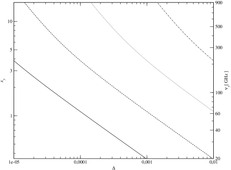
Figure 1: ${\hat{x}}_{y}$ as a function of $\Delta$ for different values of $\epsilon$ according to equation (11): For $\epsilon=10^{-5}$ (solid), $\epsilon=10^{-4}$ (dashed), $\epsilon=10^{-3}$ (dotted) and $\epsilon=10^{-2}$ (dashed-dotted). The right ordinate corresponds to $\nu_{y}=k\,T_{0}\cdot{\hat{x}}_{y}/h$, with $T_{0}=2.725\,$K.

$$g_{y}({\hat{x}}_{y})=\frac{2\,\epsilon}{|\Delta|}$$ (11)

and above which the contribution of the y-distortion relative to the first order term becomes bigger than $\epsilon$. The value of $\epsilon$ is directly related to the sensitivity of the experiments. In Fig. 1 ${\hat{x}}_{y}$ has been calculated for different $\epsilon$. At frequencies lower than ${\hat{x}}_{y}$ the relation (7) is exact within the sensitivity of the experiment, whereas for ${\hat{x}}>{\hat{x}}_{y}$ the second order correction has to be taken into account. In the regime ${\hat{x}}_{y}\gtrsim 4$ for estimates the simple approximation ${\hat{x}}_{y}=2\,\epsilon/|\Delta|+2$ may be used.

To give an example, the biggest temperature fluctuation on the whole CMB sky is due to the CMB dipole. Comparing the maximum and the minimum of the dipole corresponds to $\Delta\sim 2.48\cdot 10^{-3}$. If some CMB experiment is able to accurately measure temperature fluctuations on the level of $\mu$K, contributions of $\epsilon\sim 10^{-4}$ relative to the dipole signal can be distinguished leading to ${\hat{x}}_{y,\rm d}\sim 1$. This estimate shows, that at high frequencies spectral distortions introduced by the usage of the relation (7) for the dipole anisotropy should be taken into account in future CMB missions like Planck and Act. In Sect. 5 we will discuss these distortions due to the dipole in more detail.

Let us note here, that the temperature difference should not be larger than a few percent of the temperature of the reference blackbody. Otherwise corrections due to higher orders in $\Delta$ will become important and lead to additional distortions (see Sect. 3). Fortunately, the temperature differences on the CMB sky are sufficiently small to neglect these corrections.

Equation (10) also shows, that in general the inferred temperature difference is frequency dependent. At frequencies below ${\hat{x}}_{y}$ the inferred temperature difference is close to the true temperature difference $\Delta$ and frequency independent within the sensitivity of the experiment. In this case, we will speak about a temperature distortion or fluctuation, emphasizing that it is frequency independent. It is possible to eliminate the temperature distortion using multifrequency measurements. For ${\hat{x}}>{\hat{x}}_{y}$ frequency dependent terms become important, which we will henceforth call spectral distortions.

3 Small spectral distortions due to the superposition of blackbodies

When the CMB sky is observed with finite angular resolution or equivalently if the brightness of parts of the sky (not necessarily connected) are averaged one is dealing with the sum and more generally with the superposition of blackbodies. Here we develop a general formalism to calculate the spectral distortions arising for arbitrary temperature distribution functions in the limit of small temperature fluctuations and derive criteria for the applicability of this approximation. We first discuss the basic equations necessary to describe the spectrum of the sum of blackbodies (SB) as compared to some arbitrary reference blackbody (Sect. 3.1) and then generalize these results to the superposition of blackbodies (Sect. 3.2).

3.1 Sum of blackbodies

Following the paper of Zeldovich, Illarionov & Sunyaev (1972) we express the total spectrum resulting for the SB with different temperatures $T$ as:

$$I(\nu)=\int R(T)\,B_{\nu}(T){\,\rm d}T\,.$$ (12)

Here $R(T)$ denotes the normalized ($\int R{\,\rm d}T=1$, $R\geq 0$) temperature distribution function, which will be used below to model the beam of some CMB experiment, and $B_{\nu}(T)$ is a Planck spectrum of temperature $T$ as given by equation (3). Now we want to compare the spectrum $I(\nu)$ to a reference blackbody of temperature $T_{\rm ref}$. Defining $\delta=(T-T_{\rm ref})/T_{\rm ref}$ and inserting $T=T_{\rm ref}\,(1+\delta)$ into equation (3), $B_{\nu}$ may be rewritten as

$$B_{\nu}(\delta)=A\,T_{\rm ref}^{3}\,\frac{{\hat{x}}^{3}}{e^{{\hat{x}}/(1+\delta)}-1}$$ (13)

where ${\hat{x}}=h\nu/k\,T_{\rm ref}$ is the dimensionless frequency and $A=8\pi k\,^{3}/h^{2}\,c^{2}$. CMB temperature fluctuations are of the order $\Delta T/T\sim 10^{-5}-10^{-3}$. Therefore we are interested in the case when $|\delta|\ll 1$. This allows us to perform a Taylor expansion of equation (13):

$$B_{\nu}(\delta)=\left.B_{\nu}\right|_{\delta=0}\\ -\delta\cdot{\hat{x}}\left.\frac{\displaystyle\partial B_{\nu}}{\displaystyle\partial\xi}\right|_{\delta=0}+\frac{\delta^{2}}{2}\cdot{\hat{x}}\,\left[{\hat{x}}\,\frac{\displaystyle\partial^{2}B_{\nu}}{\displaystyle\partial{\xi}^{2}}+2\,\frac{\displaystyle\partial B_{\nu}}{\displaystyle\partial\xi}\right]_{\delta=0}\\ -\frac{\delta^{3}}{6}\cdot{\hat{x}}\,\left[{\hat{x}}^{2}\,\frac{\displaystyle\partial^{3}B_{\nu}}{\displaystyle\partial{\xi}^{3}}+6\,{\hat{x}}\,\frac{\displaystyle\partial^{2}B_{\nu}}{\displaystyle\partial{\xi}^{2}}+6\,\frac{\displaystyle\partial B_{\nu}}{\displaystyle\partial\xi}\right]_{\delta=0}\\ +\frac{\delta^{4}}{24}\cdot{\hat{x}}\,\left[{\hat{x}}^{3}\,\frac{\displaystyle\partial^{4}B_{\nu}}{\displaystyle\partial{\xi}^{4}}+12\,{\hat{x}}^{2}\,\frac{\displaystyle\partial^{3}B_{\nu}}{\displaystyle\partial{\xi}^{3}}\right.\\ \left.+36\,{\hat{x}}\,\frac{\displaystyle\partial^{2}B_{\nu}}{\displaystyle\partial{\xi}^{2}}+24\,\frac{\displaystyle\partial B_{\nu}}{\displaystyle\partial\xi}\right]_{\delta=0}+\mathcal{O}(\delta^{5})\,,$$ (14)

where here $\xi={\hat{x}}/(1+\delta)$ was defined. Keeping only terms up to fourth order in $\delta$ this simplifies to:

$$B_{\nu}(\delta)=I_{\rm ref}\,\sum^{4}_{k=0}g_{k}({\hat{x}})\,\delta^{k}\,.$$ (15)

Here we used the abbreviation $I_{\rm ref}=B_{\nu}(\delta=0)$ for the reference blackbody spectrum of temperature $T_{\rm ref}$ and defined the functions $g_{k}({\hat{x}})$ as

$$g_{0}({\hat{x}}) =1$$ (16a)

$$g_{1}({\hat{x}}) =\frac{{\hat{x}}\,e^{{\hat{x}}}}{e^{{\hat{x}}}-1}$$ (16b)

$$g_{2}({\hat{x}}) =\frac{g_{1}}{2}\left[{\hat{x}}\,\frac{e^{{\hat{x}}}+1}{e^{{\hat{x}}}-1}-2\right]\equiv\frac{g_{1}}{2}\cdot g_{y}({\hat{x}})$$ (16c)

$$g_{3}({\hat{x}}) =g_{1}\left[\frac{{\hat{x}}^{2}}{6}\,\frac{\cosh{{\hat{x}}}+2}{\cosh{{\hat{x}}}-1}-\frac{2g_{2}}{g_{1}}-1\right]$$ (16d)

$$g_{4}({\hat{x}}) =g_{1}\left[\frac{{\hat{x}}^{3}}{24}\,\frac{6\coth{\frac{{\hat{x}}}{2}}+\sinh{{\hat{x}}}}{\cosh{{\hat{x}}}-1}-3\,\frac{g_{2}+g_{3}}{g_{1}}-1\right]$$ (16e)

where $g_{y}({\hat{x}})$ is defined by equation (5). In Fig. 2 the frequency dependence of the functions $g_{i}({\hat{x}})$ is illustrated. Deviations from a blackbody spectrum become most important in the Wien region and vanish in the RJ region of the CMB spectrum.

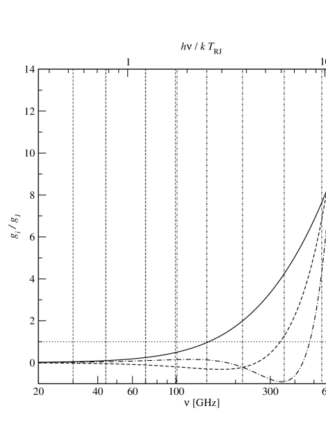
Figure 2: Frequency dependence of $g_{i}/g_{1}\equiv\Delta T_{i}/T_{\rm RJ}\,\delta^{i}$: Dotted line $\Delta T_{1}/T_{\mathrm{RJ}}\,\delta$, which is equivalent to a temperature distortion, solid line $g_{y}({\hat{x}})=2\Delta T_{2}/T_{\mathrm{RJ}}\,\delta^{2}$, which is equivalent to a y-distortion $\Delta T/y\,T_{0}$ as given by equation (5), dashed line $\Delta T_{3}/T_{\mathrm{RJ}}\,\delta^{3}$ and dashed-dotted line $\Delta T_{4}/T_{\mathrm{RJ}}\,\delta^{4}$. The function $g_{y}({\hat{x}})$ becomes larger than unity for $\nu\geq 146.2\,$ GHz or ${\hat{x}}\geq 2.57$, larger than 5 for $\nu\geq 396.7\,$GHz or ${\hat{x}}\geq 6.99$ and larger than 10 for $\nu\geq 681.3\,$GHz or ${\hat{x}}\geq 12$. For $\nu=100\,$ GHz or ${\hat{x}}=1.76$ it follows $g_{y}=0.5$. Also shown as vertical lines are the Planck LFI (dashed) and HFI (dash-dotted) frequency channels.

Inserting equation (15) into (12) the relative difference $\Delta I/I_{\rm ref}=(I-I_{\rm ref})/I_{\rm ref}$ between the SB spectrum and the reference blackbody $I_{\rm ref}$ can be derived

$$\frac{\Delta I}{I_{\rm ref}}\approx\sum^{4}_{k=1}g_{k}({\hat{x}})\,\left<\delta^{k}\right>\,,$$ (17)

where we introduced the abbreviation $\left<\delta^{k}\right>=\int R\,\delta^{k}{\,\rm d}T$ for the $k$-th moment of the temperature distribution. To find the corresponding difference in temperatures from (17) one may use the relation (7). As mentioned before the inferred temperature difference in general will be frequency dependent.

In equation (17) the term proportional to the first moment, $\left<\delta^{1}\right>$, corresponds to a temperature distortion which introduces a frequency independent shift in the measured temperature difference. It is possible to eliminate this contribution by multifrequency measurements, since it does not change with frequency. The term proportional to the second moment is indistinguishable from a Compton y-distortion as given by equation (4) with y-parameter

$$y_{\rm S}=\frac{\left<\delta^{2}\right>}{2}\,.$$ (18)

Higher moments lead to additional spectral distortions making the total spectral distortion differ from a pure y-distortion. As will be shown below for the CMB these higher order corrections can be neglected.

Limiting cases for $\frac{\Delta T}{T_{\rm ref}}$

In the RJ limit (${\hat{x}}\ll 1$), starting from (12) and using relation (7) one can find

$$\left.\frac{\Delta T}{T_{\rm ref}}\right|_{\rm RJ} \stackrel{{\scriptstyle\stackrel{{\scriptstyle{\hat{x}}\ll 1}}{{\downarrow}}}}{{\approx}}\left<\delta\right>+\frac{{\hat{x}}^{2}}{12}\left<\frac{\delta^{2}}{1+\delta}\right>$$ (19a)

$$\!\!\!\!\!\stackrel{{\scriptstyle\stackrel{{\scriptstyle{\hat{x}}\ll 1\wedge\delta\ll 1}}{{\downarrow}}}}{{\approx}}\left<\delta\right>+\frac{{\hat{x}}^{2}}{12}\Big{[}\left<\delta^{2}\right>-\left<\delta^{3}\right>+\left<\delta^{4}\right>\Big{]}\,.$$ (19b)

This result shows, that for ${\hat{x}}\rightarrow 0$ the functions $g_{2}$, $g_{3}$, and $g_{4}$ all vanish like $\sim x^{2}$, reflecting the fact that the sum of RJ spectra is again a RJ spectrum and that no spectral distortions are expected for ${\hat{x}}\ll 1$. In the first step we have only assumed that ${\hat{x}}\ll 1$. Therefore, up to second order in ${\hat{x}}$ equation (19a) describes the SB for any $\delta$ to very high accuracy. For $\delta\gg 1$ equation (19a) takes the form $\Delta T/T_{\rm ref}|_{\rm RJ}\approx\left<\delta\right>\cdot[1+\frac{{\hat{x}}^{2}}{12}]$. For the approximation (19b) we have in addition to ${\hat{x}}\ll 1$ assumed that $\delta\ll 1$. In this limit the same result can be obtained starting from equation (17).

In the Wien region of the CMB spectrum (${\hat{x}}\gg 1$) again starting from (12) and using relation (7) one can deduce

$$\left.\frac{\Delta T}{T_{\rm ref}}\right|_{\rm W} \stackrel{{\scriptstyle\stackrel{{\scriptstyle{\hat{x}}\gg 1}}{{\downarrow}}}}{{\approx}}\frac{1}{x}\cdot\left[\left<\exp\left(x\cdot\frac{\delta}{1+\delta}\right)\right>-1\right]$$ (20a)

$$\!\!\!\!\!\!\!\stackrel{{\scriptstyle\stackrel{{\scriptstyle{\hat{x}}\gg 1\wedge x\cdot\delta\ll 1}}{{\downarrow}}}}{{\approx}}\left<\delta\right>-\left<\delta^{2}\right>+\left<\delta^{3}\right>-\left<\delta^{4}\right>$$

$$\qquad\quad+\frac{{\hat{x}}}{2}\left[\left<\delta^{2}\right>+\frac{{\hat{x}}}{3}\,\left<\delta^{3}\right>+\frac{{\hat{x}}^{2}}{12}\,\left<\delta^{4}\right>\right]\,.$$ (20b)

Equation (20a) is valid for ${\hat{x}}\gg 1$ and arbitrary $\delta$, whereas (20) only is applicable for ${\hat{x}}\gg 1$ and $x\cdot\delta\ll 1$. Result (20) can be also obtained starting from equation (17).

When higher order moments are important

Using multifrequency observations it is possible to eliminate the temperature distortion ($\propto\left<\delta\right>$). In this case, the leading term in the signal corresponds to the y-distortion. Here we are interested in the question when higher order moments start to contribute significantly to the total spectral distortions. In the RJ region using equation (19b) one can find that for

$$\epsilon\cdot\left<\delta^{2}\right>>|\left<\delta^{3}\right>-\left<\delta^{4}\right>|$$ (21)

the relative contributions of the higher moments to the y-distortion is less than $\epsilon$. This equation shows, that in general corrections due to the higher moments will be of the order of $\sim|\left<\delta^{3}\right>|/\left<\delta^{2}\right>$. For temperature distributions which are symmetric around the reference temperature all the odd moments vanish. In this case the corrections typically will be of the order of $\sim\left<\delta^{4}\right>/\left<\delta^{2}\right>$. If we consider the simple case, when we compare two pure blackbodies with temperatures $T_{1}$ and $T_{2}$ and use $T_{\rm ref}=T_{1}$ then the moments are given as $\left<\delta^{k}\right>=\Delta^{k}$, with $\Delta=(T_{2}-T_{1})/T_{1}$. From this we can conclude, that the relative contribution of the third moment to the spectral distortion will be $\lesssim|\Delta|$. Therefore, in the RJ region of the spectrum even for $\Delta\sim 10^{-2}$ higher order moments will lead to corrections $\lesssim 1\%$ to the y-distortion. For the CMB with $\Delta\sim 10^{-5}-10^{-3}$ these corrections can be safely neglected.

In the Wien region the situation is a bit more complicated. Given some value of $\epsilon$ one can find the frequency $\hat{x}_{\rm c}$ above which the relative contribution of higher order moments will become important. To find $\hat{x}_{\rm c}$ one has to solve the non-linear equation

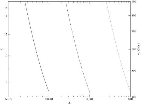
Figure 3: ${\hat{x}}_{y}$ as a function of $\Delta$ for different values of $\epsilon$ according to equation (22) assuming that $\left<\delta^{k}\right>=\Delta^{k}$: For $\epsilon=10^{-4}$ (solid), $\epsilon=10^{-3}$ (dashed) and $\epsilon=10^{-2}$ (dotted). The right ordinate corresponds to $\nu_{y}=k\,T_{0}\cdot{\hat{x}}_{y}/h$, with $T_{0}=2.725\,$K.

$$\epsilon =\frac{g_{3}(\hat{x}_{\rm c})\left<\delta^{3}\right>+g_{4}(\hat{x}_{\rm c})\left<\delta^{4}\right>}{g_{2}(\hat{x}_{\rm c})\left<\delta^{2}\right>}$$ (22)

or an equivalent equation directly using (12). In Fig. 3 $\hat{x}_{\rm c}$ has been calculated for different $\epsilon$ and $\Delta$ again considering the simple case, when we compare two pure blackbodies with temperatures $T_{1}$ and $T_{2}$ and use $T_{\rm ref}=T_{1}$. Higher order moments contribute 1% to the total spectral distortion above $\hat{x}_{\rm c}=10$ for $\Delta\sim 5\cdot 10^{-3}$, which is roughly 5 times the dipole amplitude. For $|\Delta|\lesssim 3\cdot 10^{-3}$ corrections are less than $1\%$ even in the highest Planck frequency channels. In the limit $\hat{x}_{\rm c}\gtrsim 6$ for estimates of the critical frequency above which higher order correction become bigger than $\epsilon$ one may use

$$\hat{x}_{\rm c}=\min\left[3\,\epsilon\,\frac{\left<\delta^{2}\right>}{|\left<\delta^{3}\right>|}+4,\sqrt{12\,\epsilon\,\frac{\left<\delta^{2}\right>}{\left<\delta^{4}\right>}}+5\,\right]\,.$$ (23)

In summary, the above discussion shows that, as long as $|\Delta|<\epsilon$ the spectral distortion for ${\hat{x}}<\hat{x}_{\rm c}$ is given by a pure y-distortion. In this case the biggest deviations from a y-distortion are expected in the Wien region of the CMB spectrum, where the sensitivity of the Planck mission and other future experiments is high. But even for the dipole anisotropy these corrections should be less than 1%. If $|\Delta|\sim\epsilon$ deviations in the RJ become important and higher order corrections have to be taken into account. Given the amplitude of the temperature fluctuations on the CMB sky, $\Delta\sim 10^{-5}-10^{-3}$, corrections to the y-distortion due to higher moments will be less than 1% in the highest Planck frequency channels even for the dipole amplitude and certainly less than $0.1\%$ for the higher multipoles. Therefore we can safely describe the spectral distortions arising due to the superposition of blackbodies with slightly different temperatures by y-distortions. In what follows below we assume that higher order corrections are negligible.

Beam spectral distortion

In the RJ limit the sum of blackbodies (SB) is again a blackbody with temperature $T_{\mathrm{RJ}}=\int R\,T{\,\rm d}T$. The RJ temperature $T_{\mathrm{RJ}}$ can be directly measured at sufficiently low frequencies and hence it is convenient to compare the SB to a reference blackbody of temperature $T_{\mathrm{RJ}}$. This makes any distortion due to the SB vanish at low $\nu$.

In the following, we will call $\left<\delta^{k}\right>$ beam moment, when $\delta=(T-T_{\mathrm{RJ}})/T_{\mathrm{RJ}}$ is defined as the relative difference between the temperature $T$ of a given blackbody inside the beam and the RJ temperature of the SB, i.e. the beam RJ temperature $T_{\mathrm{RJ}}$. For this choice of reference blackbody the temperature distortion vanishes and we obtain

$$\frac{\Delta I}{\bar{I}}\approx g_{2}({\hat{x}})\,\left<\delta^{2}\right>\,,$$ (24)

where ${\hat{x}}=h\nu/k\,T_{\mathrm{RJ}}$ and we introduced $\bar{I}=B_{\nu}(T_{\mathrm{RJ}})$. We should mention again that the beam spectral distortion arising due to the SB with different temperatures can be approximated by a pure y-distortion with y-parameter $y_{\rm S}$ as given by (18), if only the second moment of the temperature distribution, $\left<\delta^{2}\right>$, is important. In general higher moments have to be taken into account leading to additional spectral distortions.

Sum of two Planck spectra with different weights

For the sum of two Planck spectra with temperatures $T_{1}$ and $T_{2}$ of relative weights $w_{1}$ and $w_{2}=1-w_{1}$ the RJ temperature is given by $\bar{T}=w_{1}\,T_{1}+w_{2}\,T_{2}$. For the first five beam moments one may obtain:

$$\left<\delta^{0}\right> =1,\qquad\left<\delta^{1}\right>=0$$ (25a)

$$\left<\delta^{2}\right> =w_{1}\,w_{2}\cdot\left[\frac{\Delta T}{\bar{T}}\right]^{2}$$ (25b)

$$\left<\delta^{3}\right> =w_{1}\,w_{2}\,(1-2\,w_{1})\cdot\left[\frac{\Delta T}{\bar{T}}\right]^{3}$$ (25c)

$$\left<\delta^{4}\right> =w_{1}\,w_{2}\,(1-3\,w_{1}\,w_{2})\cdot\left[\frac{\Delta T}{\bar{T}}\right]^{4}\,.$$ (25d)

Here $\Delta T=T_{1}-T_{2}\neq 0$ was defined. Making use of equation (23), in general ($w_{1}\neq w_{2}\neq 0$) the spectral distortion significantly deviates from a y-distortion by a fraction $\epsilon$ at frequencies

$${\hat{x}}\geq\min\left[\frac{3\,\epsilon}{|1-2\,w_{1}|},\sqrt{\frac{12\,\epsilon}{1-3\,w_{1}\,w_{2}}}\,\right]\cdot\frac{\bar{T}}{|\Delta T|}$$ (26)

If one of the weights $w_{1}$ or $w_{2}$ vanishes then, as expected, there is no distortion. In the case $w_{1}\equiv w_{2}$, all the odd moments vanish and the even moments are given by $\left<\delta^{n}\right>=\left[\Delta T/(T_{1}+T_{2})\right]^{n}$. Then the critical frequency $\hat{x}_{\rm c}=2\cdot\sqrt{3}\cdot 10^{-1}\,(T_{1}+T_{2})/|\Delta T|$ above which the spectral distortion deviates significantly from a y-distortion becomes 10 only if $|\Delta T|\approx 0.069\,\bar{T}$. This implies that for non gaussian temperature distributions deviations from a y-distortion will only be important if the temperature difference becomes of the order of a few $\%$ of the RJ temperature. This is clearly not the case for the CMB in the observed universe. Even the dipole anisotropy leads to a y-distortion up to very high frequencies and we can safely neglect the contributions of moments of the temperature distribution with $k>2$.

Difference to an arbitrary reference blackbody

Here we want to derive the equations describing the comparison of the spectrum of the SB with an arbitrary reference blackbody. This example can be applied for absolute measurements of the CMB. Starting again from equation (17) and using the results obtained for the beam spectral distortions, one can rewrite the moments of $\delta_{\rm ref}=(T-T_{\rm ref})/T_{\rm ref}$ in terms of the beam moments, $\left<\delta^{k}\right>$ and $\Delta_{\rm RJ}=(T_{\mathrm{RJ}}-T_{\rm ref})/T_{\rm ref}$, with $\delta=(T-T_{\mathrm{RJ}})/T_{\mathrm{RJ}}$:

$$\left<\delta_{\rm ref}^{1}\right> =\Delta_{\rm RJ}$$ (27a)

$$\left<\delta_{\rm ref}^{2}\right> =\left<\delta^{2}\right>+\Delta_{\rm RJ}^{2}+\mathcal{O}\left(\left<\delta^{2}\right>\cdot\Delta_{\rm RJ}\right)\,.$$ (27b)

Using formula (17), one can directly infer the relative difference between the spectrum of the SB and the chosen reference blackbody $I_{\rm ref}=B_{\nu}(T_{\rm ref})$:

$$\frac{I-I_{\rm ref}}{I_{\rm ref}} =g_{1}({\hat{x}}_{\rm ref})\,\Delta_{\rm RJ}+g_{2}({\hat{x}}_{\rm ref})\,\left[\Delta_{\rm RJ}^{2}+\left<\delta^{2}\right>\right]\,,$$ (28)

where ${\hat{x}}_{\rm ref}=h\nu/k\,T_{\rm ref}$ and we assumed that the contributions of $\left<\delta^{2}\right>\cdot\Delta_{\rm RJ}$ and any higher moments of both $\delta$ and $\Delta_{\rm RJ}$ are negligible. Note that $g_{2}({\hat{x}}_{\rm ref})=g_{2}({\hat{x}})\cdot[1+\mathcal{O}(\Delta_{\rm RJ})$] and therefore $g_{2}({\hat{x}}_{\rm ref})\left<\delta^{2}\right>\equiv\Delta I/\bar{I}$, where $\Delta I/\bar{I}$ is given by equation (24).

Equation (28) shows that the spectral distortion of the SB spectrum with respect to the some reference blackbody $I_{\rm ref}$ has the following three contributions:

1. A temperature distortion $\propto\Delta_{\rm RJ}$. This distortion vanishes if the SB is compared to a blackbody with temperature $T_{\rm ref}=T_{\mathrm{RJ}}$. Since the y-distortion vanishes in the RJ region of the CMB spectrum $\Delta_{\rm RJ}$ can be directly measured at low frequencies.

2. A y-distortion $\propto\Delta_{\rm RJ}^{2}$ due to the dispersion of the RJ temperature of the SB with respect to the chosen reference temperature. This contribution also vanishes if the chosen reference blackbody has temperature $T_{\rm ref}=T_{\mathrm{RJ}}$.

3. A y-distortion $\propto\left<\delta^{2}\right>$ due to the dispersion of the temperature $T$ with respect to the RJ temperature of the SB. Only if the temperature distribution function is a Dirac $\delta$-function, i.e. when all the blackbodies inside the beam have the same temperature or equivalently when the angular resolution of the experiment is infinite, this term vanishes. For the SB it sets the minimal value of the y-parameter for a given temperature distribution function.

Equation (28) represent the most general case for the comparison of the SB with any reference blackbody in the limit of small temperature fluctuations around the temperature of the reference blackbody. It implies that in this limit the y-distortion arising due to the comparison of the SB spectrum with some chosen reference blackbody with temperature $T_{\rm ref}$ is completely determined by the second beam moment and the beam RJ temperature.

3.2 Superposition of Planck spectra

Using the results obtained so far, it is possible to generalized the sum of Planck spectra to the superposition of Planck spectra. This case applies for differential measurements of the CMB, where we directly compare two identical beams with intensities $I_{1}$ and $I_{2}$ and measure the intensity difference $\Delta I=I_{2}-I_{1}$. If we want to apply the relation (7) to relate $\Delta I\leftrightarrow\Delta T$ then we have to fix the reference temperature $T_{\rm ref}$ and thereby define the reference blackbody $I_{\rm ref}$. During the discussion in Sect. 2.2 we used $T_{\rm ref}=T$ (cf. equation (8)) but in principle one is free to choose any temperature for which the limit of small spectral distortions is justified, since $\Delta I=I_{2}-I_{1}=I_{2}-I_{\rm ref}+I_{\rm ref}-I_{1}$. In the case of the CMB, one will usually set $T_{\rm ref}$ equal to the whole sky mean temperature $T_{0}$, but as will be shown below the inferred y-distortion strongly depends on this choice.

Defining $\Delta_{i}=(T_{i}-T_{\rm ref})/T_{\rm ref}$, where $T_{i}$ are the temperatures of the blackbodies inside the beam $i$, and applying formula (17) one may obtain

$$\frac{I_{2}-I_{1}}{I_{\rm ref}}=g_{1}({\hat{x}})\,\left[\Delta_{\rm sup,12}+g_{y}({\hat{x}})\cdot y_{\rm sup,12}\right]\,,$$ (29)

with ${\hat{x}}=h\,\nu/k\,T_{\rm ref}$ and

$$\Delta_{\rm sup,12} =\left<\Delta_{2}\right>_{\rm b,2}-\left<\Delta_{1}\right>_{\rm b,1}=\frac{\bar{T}_{\rm b,2}-\bar{T}_{\rm b,1}}{T_{\rm ref}}$$ (30a)

$$y_{\rm sup,12} =\frac{1}{2}\left[\left<\Delta^{2}_{2}\right>_{\rm b,2}-\left<\Delta^{2}_{1}\right>_{\rm b,1}\right]\,,$$ (30b)

where $\left<X\right>_{\rm b,\it i}$ denotes the corresponding beam averages and we defined the beam RJ temperatures $\bar{T}_{\rm b,\it i}=\left<T_{i}\right>_{\rm b,\it i}$. In equation (29) we have neglected the contributions of any higher moments of $\Delta_{i}$. Here the temperature distortion is directly related to the relative difference of the RJ temperatures.

The y-parameter $y_{\rm sup,12}$ can be rewritten using the beam moments $\big{<}\delta_{i}^{2}\big{>}_{\rm b,\it i}$, with $\delta_{i}=(T_{i}-\bar{T}_{\rm b,\it i})/\bar{T}_{\rm b,\it i}$ and defining $\Delta_{\rm ref,\it i}=\left<\Delta_{i}\right>_{\rm b,\it i}=(\bar{T}_{\rm b,\it i}-T_{\rm ref})/T_{\rm ref}$:

$$y_{\rm sup,12}=\frac{1}{2}\,\left[\left<\delta_{2}^{2}\right>_{\rm b,2}-\left<\delta_{1}^{2}\right>_{\rm b,1}\right]\\ +\frac{1}{2}\,\left[\Delta^{2}_{\rm ref,2}-\Delta^{2}_{\rm ref,1}\right]+\mathcal{O}(\left<\delta_{i}^{2}\right>_{\rm b,\it i}\cdot\Delta_{\rm ref,\it i})\,.$$ (31)

The difference of the beam moments $\big{<}\delta_{i}^{2}\big{>}_{\rm b,\it i}$ does not depend on the chosen reference temperature $T_{\rm ref}$ and therefore always leads to the same contribution

$$y_{\rm b}=\frac{1}{2}\,\left[\left<\delta_{2}^{2}\right>_{\rm b,2}-\left<\delta_{1}^{2}\right>_{\rm b,1}\right]$$ (32)

to the inferred y-parameter. In the limit of high angular resolution it vanishes. For the second term in (31) ($\propto\Delta^{2}_{\rm ref,2}-\Delta^{2}_{\rm ref,1}$) one finds

$$y_{12}(T_{\rm ref})=\frac{1}{2}\,\left[\Delta^{2}_{\rm ref,2}-\Delta^{2}_{\rm ref,1}\right]=\Delta_{\rm sup,12}\cdot\Delta_{\rm RJ}\,,$$ (33)

with $\Delta_{\rm RJ}=(T_{\mathrm{RJ}}-T_{\rm ref})/T_{\rm ref}$ and $T_{\mathrm{RJ}}=(\bar{T}_{\rm b,1}+\bar{T}_{\rm b,2})/2$. This contribution to the total inferred y-parameter, $y_{\rm sup,12}(T_{\rm ref})=y_{\rm b}+y_{12}(T_{\rm ref})$, depends on the choice of $T_{\rm ref}$. Here it becomes clear that setting $T_{\rm ref}\equiv T_{\mathrm{RJ}}$, i.e. to the average RJ temperature of the sum of both beams, only the difference of the second beam moments leads to a y-distortion. Let us note here, that equation (28) is a special case of (29), where beam 1 has no contribution of the beam moment $\left<\delta_{1}^{2}\right>_{\rm b,1}$, i.e. where the beam spectrum is a blackbody with temperature $\bar{T}_{\rm b,1}$, and where $T_{\rm ref}=\bar{T}_{\rm b,1}$.

Dependence on the reference temperature

Here we want to clarify some aspects of the dependence of the inferred y-parameter on the chosen reference temperature. If we assume that $y_{\rm b}\ll 1$ and $\bar{T}_{\rm b,2}>\bar{T}_{\rm b,1}$, we can find the reference temperature at which the total y-distortion vanishes:

$$T_{y=0}=\frac{\bar{T}_{\rm b,1}+\bar{T}_{\rm b,2}}{2}\,\left[1+\frac{\bar{T}_{\rm b,1}+\bar{T}_{\rm b,2}}{\bar{T}_{\rm b,2}-\bar{T}_{\rm b,1}}\cdot\frac{y_{\rm b}}{2}\right]\,.$$ (34)

In the limit of high angular resolution ($y_{\rm b}=0$) we find that $T_{y=0}=T_{\mathrm{RJ}}$. One encounters this situation in differential measurements of the CMB brightness between two points on the sky. For $\bar{T}_{\rm b,2}>\bar{T}_{\rm b,1}$ and $y_{\rm b}>0$ the reference temperature at which the y-distortion vanishes is always positive and also the temperature distortion corresponding to the first term in equation (29) is positive. Then for the inferred y-distortion the following three regimes can be defined: (i) for $T_{\rm ref}<T_{y=0}$ the inferred y-distortion is positive, (ii) for $T_{\rm ref}=T_{y=0}$ per definition there is no y-distortion up to first order in $y_{\rm b}$ and (iii) for $T_{\rm ref}>T_{y=0}$ the inferred y-distortion is negative even though $\bar{T}_{\rm b,2}>\bar{T}_{\rm b,1}$. This shows that for the superposition of Planck spectra it is in general not sufficient to choose the beam intensity with higher RJ temperature as $I_{2}$ in order to obtain a positive y-parameter.

Now we are interested in the change of $\Delta_{\rm sup,12}$ and $y_{\rm sup,12}$, if we change from one reference temperature $T_{\rm ref}$ to another $T^{\prime}_{\rm ref}$. For $T^{\prime}_{\rm ref}$ one can again write down an equation similar to (29), where now $\Delta_{i}=(T_{i}-T_{\rm ref})/T_{\rm ref}$ is replaced by $\Delta^{\prime}_{i}=(T_{i}-T^{\prime}_{\rm ref})/T^{\prime}_{\rm ref}$ and ${\hat{x}}=h\nu/k\,T_{\rm ref}$ by ${\hat{x}}^{\prime}=h\nu/k\,T^{\prime}_{\rm ref}$. Using (30) and (31), we can write

$$\Delta_{\rm sup,12}^{\prime} =\frac{T_{2}-T_{1}}{T^{\prime}_{\rm ref}}=\Delta_{\rm sup,12}\cdot[1+\Delta_{\rm r}]$$ (35a)

$$y_{\rm sup,12}^{\prime} =y_{\rm b}^{\prime}+y_{12}^{\prime}(T^{\prime}_{\rm ref})\stackrel{{\scriptstyle\stackrel{{\scriptstyle y_{\rm b}^{\prime}\equiv y_{\rm b}}}{{\downarrow}}}}{{=}}y_{\rm b}+\Delta_{\rm sup,12}^{\prime}\cdot\Delta_{\rm RJ}^{\prime}$$

$$=y_{\rm b}+\Delta_{\rm sup,12}\cdot[1+\Delta_{\rm r}]\cdot[\Delta_{\rm RJ}\,(1+\Delta_{\rm r})+\Delta_{\rm r}]$$ (35b)

$$\approx y_{\rm b}+y_{12}+\Delta_{\rm sup,12}\cdot\Delta_{\rm r}\,,$$ (35c)

with $\Delta_{\rm r}=(T_{\rm ref}-T^{\prime}_{\rm ref})/T^{\prime}_{\rm ref}$ and where prime denotes, that the reference temperature $T^{\prime}_{\rm ref}$ was used. The difference of y-parameters is given by $\Delta y=y_{\rm sup,12}^{\prime}-y_{\rm sup,12}=\Delta_{\rm sup,12}\cdot\Delta_{\rm r}$. For $T_{\rm ref}=T_{\mathrm{RJ}}$ the contribution $y_{12}=0$. Therfore we can write the inferred y-parameter for any reference temperature as:

$$y(T_{\rm ref})\approx y_{\rm b}+\frac{\bar{T}_{\rm b,2}-\bar{T}_{\rm b,1}}{\bar{T}_{\rm b,1}+\bar{T}_{\rm b,2}}\cdot\frac{\bar{T}_{\rm b,1}+\bar{T}_{\rm b,2}-2\,T_{\rm ref}}{T_{\rm ref}}\,.$$ (36)

This result describes all the cases discussed previously: If we want to discuss the beam distortions we have to set the reference temperature to $T_{\mathrm{RJ}}$ making $y\approx y_{\rm b}$. If we are discussing the y-parameter for the comparison of the SB with some reference blackbody we have $\bar{T}_{\rm b,1}=T_{\rm ref}$ resulting in $y\approx y_{\rm b}+\Delta_{\rm RJ}^{2}/2$. This implies that in the limit of small spectral distortions the y-parameter for the superposition of Planck spectra is completely determined by the second beam moments and the beam RJ temperatures.

4 Superposition of two Planck spectra

In order to illustrate the main results obtained in the previous Sect. we now discuss the spectral distortions arising due to the sum and difference of two pure blackbodies with different temperatures $T_{1}$ and $T_{2}$ and the corresponding intensities $I_{1}=B_{\nu}(T_{1})$ and $I_{2}=B_{\nu}(T_{2})$ in the presence of a reference blackbody $I_{\rm ref}=B_{\nu}(T_{\rm ref})$ with temperature $T_{\rm ref}$. In principle one can directly apply the results obtained in Sect. 3 and easily derive the equations describing this situation, but in order to check the derivations of the previous Sect. we here choose an approach starting from the expansion (9) taking only first order corrections into account. Since the CMB temperature fluctuations are very small this approximation is sufficient.

The results obtained for the sum of two blackbodies apply to the case of an absolute measurement of the CMB sky, where the beam contains only blackbodies with two equally weighted temperatures. In the limit of narrow beams the results obtained for the difference of two blackbodies can be directly used to discuss the effects arising in differential measurements. In Sect. 8 we will use some of the result of this Sect. in the discussion about cross calibration issues.

4.1 Sum of two Planck spectra

We want to describe the difference $\Delta I_{\rm S}=I_{\rm S}-I_{\rm ref}$, as a function of frequency. Here we defined the sum of the two blackbodies by $I_{\rm S}=(I_{1}+I_{2})/2$. The easiest is to first calculate the difference $\Delta I_{i}=I_{i}-I_{\rm ref}$ since $\Delta I_{\rm S}\equiv(\Delta I_{1}+\Delta I_{2})/2$. If we define $\Delta_{i}=(T_{i}-T_{\rm ref})/T_{\rm ref}$ and ${\hat{x}}=h\nu/k\,T_{\rm ref}$ we can make use of equation (9) and write the relative difference of $I_{\rm S}$ and $I_{\rm ref}$ as

$$\frac{I_{\rm S}-I_{\rm ref}}{I_{\rm ref}} \approx\frac{{\hat{x}}\,e^{\hat{x}}}{e^{\hat{x}}-1}\cdot\left[\frac{\Delta_{1}+\Delta_{2}}{2}+g_{y}({\hat{x}})\cdot\frac{y_{1}+y_{2}}{2}\right]\,.$$ (37)

Here we abbreviated the y-parameters as $y_{i}=\Delta^{2}_{i}/2$. Defining the RJ temperature $T_{\mathrm{RJ}}=(T_{1}+T_{2})/2$ of the sum of the two blackbodies, the sum of the first order terms and the y-parameters may be rewritten like

$$\Delta_{\rm RJ} =\frac{\Delta_{1}+\Delta_{2}}{2}=\frac{T_{\mathrm{RJ}}-T_{\rm ref}}{T_{\rm ref}}$$ (38a)

$$y_{\rm sum} =\frac{y_{1}+y_{2}}{2}\approx\frac{1}{2}\left[\Delta_{\rm RJ}^{2}+\left(\frac{T_{1}-T_{2}}{T_{1}+T_{2}}\right)^{2}\right]\,.$$ (38b)

From this it can be seen that if the reference temperature is set to $T_{\mathrm{RJ}}$ the temperature distortion corresponding to the first term in (37) vanishes ($\Delta_{\rm RJ}=0$) and only a minimal y-distortion with y-parameter

$$y_{\rm b}=\frac{1}{2}\,\left[\frac{T_{1}-T_{2}}{T_{1}+T_{2}}\right]^{2}$$ (39)

is left. At low frequencies (${\hat{x}}<{\hat{x}}_{y})$ this reflects the fact that the sum of RJ spectra is again a RJ spectrum. Comparing (38) to (27) one may conclude that $y_{\rm b}$ corresponds to the contribution of the second beam moment $\left<\delta^{2}\right>$ to the y-parameter. Comparing (39) to (25b) with $w_{1}=w_{2}=\frac{1}{2}$ confirms this conclusion.

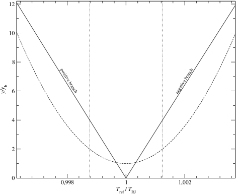
Figure 4: Dependence of the inferred y-parameter on the chosen reference temperature $T_{\rm ref}$ for two blackbodies with temperatures $T_{1}=2.72162\,$K and $T_{2}=2.72838\,$K, corresponding to the minimum and maximum of the CMB dipole. In this case the mean RJ temperature is $T_{\mathrm{RJ}}=(T_{1}+T_{2})/2=2.725\,$K and $y_{\rm b}=7.7\cdot 10^{-7}$. — Sum of two blackbodies: total y-parameter as given by (38b) (dashed line). — Difference of two blackbodies: the absolute value $|y_{\rm dif}|$ of the inferred y-parameter as given in equation (41b) (solid line). The dotted vertical lines show the location of $T_{\rm ref}=T_{1}$ and $T_{\rm ref}=T_{2}$ respectively.

The dependence of the inferred y-parameter on the chosen reference temperature is illustrated in Figure 4. As mentioned above the y-parameter reaches a minimum for $T_{\rm ref}=T_{\mathrm{RJ}}$. It is important to note that the minimal value of the y-parameter $y_{\rm b}$ does not depend on the reference temperature $T_{\rm ref}$ but only on the second beam moment of the temperature distribution function. Changing $T_{\rm ref}$ from $T_{\mathrm{RJ}}\rightarrow T_{i}$ the inferred y-parameter monotonically increases being a factor of $\sim 2$ larger than $y_{\rm b}$ for $T_{\rm ref}=T_{i}$. This can be understood as follows: If we set $T_{\rm ref}=T_{i}$ we obtain $y_{\rm sum}=(T_{1}-T_{2})^{2}/4\,T^{2}_{i}\approx(T_{1}-T_{2})^{2}/4\,T^{2}_{1}+\mathcal{O}(\Delta T^{3}/T_{1}^{3})$, with $\Delta T=T_{1}-T_{2}$. Therefore the ratio $y_{\rm sum}/y_{\rm d}\approx(T_{1}+T_{2})^{2}/2\,T^{2}_{1}\approx 2$.

Outside the region $T_{1}\leq T_{\rm ref}\leq T_{2}$ the inferred y-parameter increases further. It is in principle possible to gain large factors in the inferred y-parameter by going very far away from the RJ temperature of the SB, but at some point next order corrections will become important and therefore limit $T_{\rm ref}$ to the region where the approximation of small spectral distortions is still valid. For the CMB the most natural choices of the reference temperature are the whole sky mean temperature $T_{0}$ and the maximum or minimum of the CMB dipole. For the SB the inferred y-parameter varies from $y\sim 7.7\cdot 10^{-7}$ for $T_{\rm ref}=T_{0}$ to $y\sim 1.5\cdot 10^{-6}$ for $T_{\rm ref}=T_{1}$. The behavior of the inferred y-parameter shows, that in order to minimize the arising spectral distortion for absolute measurements it is important to use an internal calibrator with temperature close to the beam RJ temperature $T_{\mathrm{RJ}}$.

In the limit $T_{1}\rightarrow T_{2}$ we are in principle comparing one pure Planck spectrum with a reference blackbody. This case applies for an absolute measurement of the CMB sky in the limit of very narrow beams. In this case it follows that $y_{\rm b}\rightarrow 0$ and in addition $y_{\rm sum}\rightarrow 0$ for $T_{\rm ref}=T_{\mathrm{RJ}}$. Except for some changes in scales the behavior of the curve shown in Fig. 4 is unaffected.

4.2 Difference of two Planck spectra

Since $\Delta I=I_{2}-I_{1}\equiv\Delta I_{2}-\Delta I_{1}$, where $\Delta I_{i}=I_{i}-I_{\rm ref}$, applying equation (9) one can easily find

$$\frac{I_{2}-I_{1}}{I_{\rm ref}} \approx\frac{{\hat{x}}\,e^{\hat{x}}}{e^{\hat{x}}-1}\cdot\Big{[}\Delta_{2}-\Delta_{1}+g_{y}({\hat{x}})\cdot(y_{2}-y_{1})\Big{]}\,.$$ (40)

Again it is possible to simplify the difference of the first order terms and the y-parameters leading to

$$\Delta_{12} =\Delta_{2}-\Delta_{1}=\frac{T_{2}-T_{1}}{T_{\rm ref}}$$ (41a)

$$y_{\rm dif} =y_{2}-y_{1}=\Delta_{12}\cdot\Delta_{\rm RJ}\,,$$ (41b)

where $\Delta_{\rm RJ}=(T_{\mathrm{RJ}}-T_{\rm ref})/T_{\rm ref}$ and $T_{\mathrm{RJ}}=(T_{1}+T_{2})/2$. For the difference of two Plancks the temperature distortion does not vanish for any choice of the reference temperature (see equation (41a)), whereas the y-distortion changes sign at $T_{\rm ref}=T_{\mathrm{RJ}}$. As mentioned earlier, this shows that for the difference of two Planck spectra in order to obtain a positive y-parameter it is in general not sufficient to choose the intensity with higher RJ temperature as $I_{2}$. Comparing (41) to (30a) and (33) and keeping in mind that both beam moments $\left<\delta_{i}^{2}\right>_{\rm b,\it i}=0$ shows the equivalence of both approaches. In Figure 4 the dependence of the absolute value of the inferred y-parameter on the chosen reference temperature is shown. At $T_{\rm ref}=T_{i}$ the inferred y-parameter for the difference of two blackbodies is 2 times larger than in the case of the sum, $\left.(|y_{\rm dif}|/y_{\rm sum})\right|_{T_{i}}\sim 2$.

As in the case of the sum of two Plancks for $T_{\rm ref}$ outside the region $T_{1}\leq T_{\rm ref}\leq T_{2}$ the inferred y-parameter increases strongly. Again there is a limit set by the approximations of small spectral distortions. The behavior of the inferred y-parameter shows, that in order to minimize the spectral distortion arising in differential measurements it is important to choose a reference temperature close to the RJ temperature of the observed region.

5 Spectral distortions due to the CMB dipole

The largest temperature fluctuation on the observed CMB sky is connected with the CMB dipole. Its amplitude has been accurately measured by Cobe/Firas (Fixsen & Mather, 2002): $\Delta T_{\rm d}=3.381\pm 0.007$mK, corresponding to $\Delta T/T\sim 0.2\,\%$ on very large angular scales. Assuming that it is only due to the motion of the solar system with respect to the CMB rest frame it implies a velocity of $v=372\pm 1$ km/s in the direction $(l,b)=(264.14^{\circ}\pm 0.15^{\circ},48.26^{\circ}\pm 0.15^{\circ})$. In order to understand the spectral distortions arising due to the dipole, we start with the direction dependent temperature of the CMB, neglecting any intrinsic anisotropy:

$$T(\mu) =\frac{T_{0}}{\gamma[1-\beta\,\mu]}$$ (42a)

$$\!\!\stackrel{{\scriptstyle\stackrel{{\scriptstyle\beta\ll 1}}{{\downarrow}}}}{{\approx}}T_{0}\,\left[1-\frac{\beta^{2}}{6}+\beta\,\mu+\beta^{2}\left(\mu^{2}-\frac{1}{3}\right)\right]\,.$$ (42b)

Here we introduced the abbreviation $\mu=\cos\theta$, with $\theta$ being the angle between the direction of $v$ and the location on the sky. $T_{0}$ denotes the intrinsic CMB temperature, $\beta=v/c$ is the velocity in units of the speed of light and $\gamma=1/\sqrt{1-\beta^{2}}$ is the corresponding Lorentz factor. The whole sky mean RJ temperature is given by

$$\bar{T}_{\rm f}=\frac{T_{0}}{2\gamma\beta}\,\ln\left[\frac{1+\beta}{1-\beta}\right]\stackrel{{\scriptstyle\stackrel{{\scriptstyle\beta\ll 1}}{{\downarrow}}}}{{\approx}}T_{0}\,\left[1-\frac{\beta^{2}}{6}\right]\,,$$ (43)

where ’f’ denotes full sky average temperature. Equation (43) implies that due to the motion of the solar system relative to the CMB restframe the observed whole sky mean RJ temperature is $\Delta T=0.70\,\mu$K less than the intrinsic temperature $T_{0}$. The measured value of the whole sky mean temperature as given by the Cobe/Firas experiment (Fixsen & Mather, 2002) is $T_{0}=2.725\pm 0.001\,$K. Therefore this difference is still $\sim 1000$ times smaller than the current error bars and far from being measured.

Below we now discuss the spectral distortions arising due to the CMB dipole in the context of finite angular resolution. Since only the second moment of the temperature distribution is important, we will use the second order expansion of $T(\mu)$ in $\beta$ as given in equation (42b). In the last part of this section we show that, starting with equation (42a) all the results of this section can also be directly obtained by expansion of the blackbody $B_{\nu}(T(\mu))$ in terms of small $\beta$. This shows the equivalence of both approaches. Nevertheless, the big advantage of the treatment developed in Sect. 3 is that it can be applied to general temperature distributions and that the source of the y-distortion can be directly related to the second moment of the temperature distribution.

5.1 Whole sky beam spectral distortion

Defining $\delta=[T(\mu)-\bar{T}_{\rm f}]/\bar{T}_{\rm f}$, where $\bar{T}_{\rm f}$ is given by equation (43), the full sky moments can be calculated by the integrals $\left<\delta^{k}\right>_{\rm f}=\frac{1}{2}\int^{1}_{-1}\delta(\mu)^{k}{\,\rm d}\mu$. The first three moments may be found as

$$\left<\delta^{0}\right>_{\rm f} =1,\qquad\left<\delta^{1}\right>_{\rm f}=0$$ (44a)

$$\left<\delta^{2}\right>_{\rm f} =\frac{4\beta^{2}\gamma^{2}}{\Xi^{2}}-1\stackrel{{\scriptstyle\stackrel{{\scriptstyle\beta\ll 1}}{{\downarrow}}}}{{\approx}}\frac{\beta^{2}}{3}+\mathcal{O}(\beta^{4})\,,$$ (44b)

where $\Xi=\ln\!\!\big{[}\frac{1+\beta}{1-\beta}\big{]}$. With $\beta_{\rm d}=\Delta T_{\rm d}/T_{0}=1.241\cdot 10^{-3}$ one finds: $\left<\delta^{2}\right>_{\rm f}=5.1\cdot 10^{-7}$. This implies a full sky y-distortion with

$$y_{\rm d}=\frac{\beta_{\rm d}^{2}}{6}\approx 2.6\cdot 10^{-7}\,,$$ (45)

which is currently $\sim 60$ times below the Cobe/Firas upper limit. This distortion translates into a temperature difference of $\Delta T=0.7\cdot g_{y}({\hat{x}})\,\mu$K. The exact behavior of $g_{y}({\hat{x}})$ is shown in Fig. 2. We have checked that deviations from a y-distortion will become important only at extremely high frequencies (${\hat{x}}\geq 360$).

Here we want to note, that this full sky distortions arises due to the existence of the dipole anisotropy. In absolute measurements of the CMB $y_{\rm d}$ places a lower limit on the full sky y-parameter (see Sect. 3.1).

5.2 Beam spectral distortion due to the CMB dipole

Here we are interested in the angular pattern of the y-distortion induced by the SB over the dipole for an observation with a finite angular resolution and in particular in the location of the maximal y-distortion, when we compare the beam flux at different frequencies to a reference blackbody with beam RJ temperature. To model the beam we use a simple top-hat filter function

$$W(\theta^{\prime})=\begin{cases}1&\text{for $\theta^{\prime}\leq\theta_{\rm r}$,}\\ 0&\text{else,}\end{cases}$$ (46)

where the $z^{\prime}$-axis is along the beam direction and $\theta_{\rm r}$ is the radius of the top-hat in spherical coordinates.

The $k$th moment of some variable $X$ over the beam is then given by the integral

$$\left<X^{k}\right>_{\rm r}=\frac{1}{2\,\pi\,(1-\mu_{\rm r})}\int^{2\,\pi}_{0}\int^{1}_{\mu_{\rm r}}X^{k}{\,\rm d}\mu^{\prime}{\,\rm d}\phi^{\prime}\,,$$ (47)

where ’r’ denotes beam average for a top-hat of radius $\theta_{\rm r}$ and $\mu_{\rm r}=\cos\theta_{\rm r}$. Defining $\mu_{0}=\cos\theta_{0}$ and using

$$\mu=\mu_{0}\cdot\mu^{\prime}+\cos(\phi^{\prime}-\phi_{0})\,\sin(\theta_{0})\sqrt{1-\mu^{\prime 2}}\,,$$ (48)

one can calculate the beam averages of the dipole and quadrupole anisotropy

$$\left<\mu\right>_{\rm r} =\zeta_{+}\,\mu_{0}$$ (49a)

$$\left<\mu^{2}-\frac{1}{3}\right>_{\rm r} =\mu_{\rm r}\,\zeta_{+}\!\left(\mu_{0}^{2}-\frac{1}{3}\right)\,,$$ (49b)

where we introduced the abbreviation $\zeta_{\pm}=\frac{1\pm\mu_{\rm r}}{2}$. These equation will be very useful in all the following discussion.

Using formula (42b) and equations (47) and (49) the mean RJ temperature inside the beam in some direction $(\phi_{0},\theta_{0})$ relative to the dipole axis is given as

$$\bar{T}_{\rm r}=T_{0}\,\left[1-\frac{\beta^{2}}{6}+\beta\,\zeta_{+}\,\mu_{0}+\,\beta^{2}\,\mu_{\rm r}\,\zeta_{+}\!\left(\mu_{0}^{2}-\frac{1}{3}\right)\right]\,.$$ (50)

The position of the maximum and minimum is, as expected, at $\theta_{0}=0$ and $\theta_{0}=\pi$ respectively.

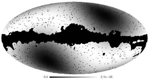
Figure 5: Angular distribution of $y_{\rm r}$ as given by equation (52) for $\theta_{\rm r}=20^{\circ}$. The maximal spectral distortion is expected to appear in a ring perpendicular to the dipole axis and in this case has a value $y_{\rm r,max}=2.3\cdot 10^{-8}$. The minimal y-parameter has a value of $y=2.4\cdot 10^{-10}$ and is located around the maximum and minimum of the dipole. The galactic plane was cut out using the kp0-mask of the Wmap data base.

Now the second moment of $\delta=[T(\mu)-\bar{T}_{\rm r}]/\bar{T}_{\rm r}$ inside the beam can be derived as:

$$\left<\delta^{2}\right>_{\rm r} \!\!\!\stackrel{{\scriptstyle\stackrel{{\scriptstyle\beta_{\rm d}\ll 1}}{{\downarrow}}}}{{\approx}}\frac{\beta^{2}_{\rm d}}{3}\cdot\left[1+\zeta_{+}-3\,\zeta_{+}\!\left(\mu_{0}^{2}-\frac{1}{3}\right)\right]\zeta_{-}\,,$$ (51)

where up to second order in $\beta$ only the CMB dipole contributes and we have set $\beta\equiv\beta_{\rm d}$. The corresponding y-parameter

$$y_{\rm r}=y_{\rm d}\cdot\left[1+\zeta_{+}-3\,\zeta_{+}\!\left(\mu_{0}^{2}-\frac{1}{3}\right)\right]\zeta_{-}\,,$$ (52)

has a monopole and quadrupole angular dependence. As expected it vanishes for high angular resolution ($\zeta_{-}\rightarrow 0$). In Fig. 5 the angular distribution of $y_{\rm r}$ for $\theta_{\rm r}=20^{\circ}$ is illustrated. The maximum lies in a broad ring perpendicular to the dipole axis, which even without taking the galaxy into account is covering a large fraction of the sky. In the shown case, the maximal value of the y-parameter is approximately $y_{\rm r,max}\sim y_{\rm d}/10$.

Using equation (51) the position of the maximum can be found: $\theta_{0,\rm max}=\frac{\pi}{2}$. This suggests that the location of the maximal distortion is where the derivative of the temperature distribution is extremal. The maximal y-parameter is given as

$$y_{\rm r,max}={y_{\rm d}}\cdot\left[1-\mu_{\rm r}\,\zeta_{+}\right]\,.$$ (53)

The dependence of $y_{\rm r,max}$ on the beam radius is shown in Fig. 6.

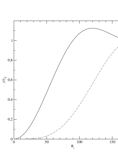
Figure 6: Dependence of the y-parameter in units of $y_{\rm d}=2.6\cdot 10^{-7}$ on the beam radius $\theta_{\rm r}$ in degree for a circular beam: $y_{\rm r}$ for $\mu_{0}=\pm 1$ as given by equation (52) (dash-dot-dotted), $y_{\rm r,max}$ according to equation (53) (solid). For values $-1<\mu_{0}<1$ the curves lie between these two extremes.

For beam radii larger than $\theta_{\rm r}=90^{\circ}$ it follows that $y_{\rm r,max}\geq{y_{\rm d}}$ and at $\theta_{\rm r}=120^{\circ}$ it is $9/8$ times ${y_{\rm d}}$. The maximal y-parameter, $y_{\rm r,max}$, is a steep function of beam radius: It has values $y_{\rm d}/2$, ${y_{\rm d}}/3$ and ${y_{\rm d}}/10$ for $\theta_{\rm r}=51.83^{\circ}$, $\theta_{\rm r}=40.68^{\circ}$ and $\theta_{\rm r}=21.29^{\circ}$ respectively and vanishes like $\sim 3\,\theta_{\rm r}^{2}/4$ for high angular resolution. For $\theta_{\rm r}=5^{\circ}$ it is $\sim 6\cdot 10^{-3}\times{y_{\rm d}}$. This implies that the beam spectral distortions resulting from the dipole are lower than $\Delta T/T\sim 10^{-9}$ for experiments with resolution better than $\sim 10^{\circ}$. As will be shown later, on this level contributions from the higher multipoles will start to become important (Sect. 6).

5.3 Distortion with respect to any $T_{\rm ref}$

We have seen in Sect. 3.1 that the inferred y-parameter for the comparison of the SB with some reference blackbody with temperature $T_{\rm ref}$ has one contribution from the second beam moment $\left<\delta^{2}\right>$ and another due to the dispersion $\Delta_{\rm RJ}^{2}$ of the beam RJ temperature relative to the temperature of the chosen reference blackbody (cf. equation (27b)). Therefore one can immediately write down the relative difference of the beam intensity and the intensity of the chosen reference blackbody making use of (27), (28), (50) and (51). In the limit $\theta_{\rm r}\rightarrow 0$ we can apply the results obtained in Sect. 4.1 for the sum of two blackbodies, if we set $T_{1}=T_{2}$. Here we want to discuss the case $T_{\rm ref}=T_{0}$ in more detail. For this choice the residual full sky y-distortion (which may be obtained by averaging the intensity data over the whole sky) is minimal.

Distortion with respect to $T_{0}$

Now, instead of comparing the spectrum of the SB to a blackbody with beam RJ temperature $\bar{T}_{\rm r}$ we compare to a blackbody of temperature $T_{0}$. Then the spectral distortion follows from equation (28) and in addition to the beam moment (51) the first two moments of $\Delta=(\bar{T}_{\rm r}-T_{0})/T_{0}$ have to be calculated:

$$\Delta^{1} =-\frac{\beta^{2}_{\rm d}}{6}+\beta_{\rm d}\,\zeta_{+}\,\mu_{0}+\,\beta_{\rm d}^{2}\,\mu_{\rm r}\,\zeta_{+}\!\left(\mu_{0}^{2}-\frac{1}{3}\right)$$ (54a)

$$\Delta^{2} =\;\;\,\frac{\beta^{2}_{\rm d}}{3}\,\zeta_{+}^{2}+\beta^{2}_{\rm d}\,\zeta_{+}^{2}\!\left(\mu_{0}^{2}-\frac{1}{3}\right)\,.$$ (54b)

The spectral distortion arising from the SB can now be characterized as follows: (i) At low frequencies the y-distortion vanishes. The motion of the solar system with respect to the CMB restframe induces a temperature dipole ($\sim\beta_{\rm d}$) and a temperature monopole and quadrupole ($\sim\beta^{2}_{\rm d}$) all resulting from the $\Delta^{1}$-term:

$$\left.\frac{\Delta T}{T_{0}}\right|_{\rm t}=-\frac{\beta^{2}_{\rm d}}{6}+\beta_{\rm d}\,\zeta_{+}\,\mu_{0}+\,\beta_{\rm d}^{2}\,\mu_{\rm r}\,\zeta_{+}\!\left(\mu_{0}^{2}-\frac{1}{3}\right)\,.$$ (55)

In the limit of high angular resolution ($\zeta_{+},\mu_{\rm r}\rightarrow 1$) this is equivalent to the expansion (42b). (ii) A y-distortion is induced which is proportional to the sum $\Delta^{2}+\left<\delta^{2}\right>_{\rm r}$:

$$\left.\frac{\Delta T}{T_{0}}\right|_{\rm y}=\frac{g_{2}({\hat{x}})}{g_{1}({\hat{x}})}\,\left[\frac{\beta^{2}_{\rm d}}{3}+\,\beta_{\rm d}^{2}\,\mu_{\rm r}\,\zeta_{+}\!\left(\mu_{0}^{2}-\frac{1}{3}\right)\right]\,.$$ (56)

It has a monopole and quadrupole angular dependence and only arises due to the CMB dipole. The sum of both contributions mentioned above can be rewritten as

$$\left.\frac{\Delta T}{T_{0}}\right|_{\rm tot} =\Delta-\Delta^{2}-\left<\delta^{2}\right>_{\rm r}+\frac{g({\hat{x}})}{2}\,\left[\Delta^{2}+\left<\delta^{2}\right>_{\rm r}\right]$$ (57a)

$$=-\frac{\beta^{2}_{\rm d}}{2}+\beta_{\rm d}\,\zeta_{+}\,\mu_{0}$$

$$\qquad+\frac{g({\hat{x}})}{2}\,\left[\frac{\beta^{2}_{\rm d}}{3}+\,\beta_{\rm d}^{2}\,\mu_{\rm r}\,\zeta_{+}\!\left(\mu_{0}^{2}-\frac{1}{3}\right)\right]\,,$$ (57b)

where we used the definition (6) for $g({\hat{x}})$. Rewriting the function $g_{2}({\hat{x}})$ in terms of $g({\hat{x}})$ lead to exact cancellation of the motion induced temperature quadrupole and changes the temperature monopole by $\beta_{\rm d}^{2}/3$ (cf. $\Delta-\Delta^{2}-\left<\delta^{2}\right>_{\rm r}$-term in equation (57a)).

Here we want to note, that in the picture of the SB it is easily understandable, that there is no difference in the resulting spectral distortion whether the dipole anisotropy is intrinsic or due to motion. Therefore, as has been noted earlier by Kamionkowski & Knox (2003), it is impossible to distinguish the intrinsic dipole from a motion induced dipole by measurement of the frequency dependent temperature quadrupole.

Expansion of $\Delta I/I_{0}$ for small $\beta$

Here we want to show, that the results (51) and (57) can also be directly obtained starting with the expansion of the blackbody spectrum with temperature $T(\mu)$ for small velocity $\beta$ and thereby prove the equivalence and correctness of both approaches. For this, inserting (42a) into the blackbody spectrum (3), by Taylor expansion up to second order of $\beta$ one may find

$$\frac{\Delta I}{I_{0}}=\beta^{2}\,g_{1}({\hat{x}})\,\left[\frac{g({\hat{x}})}{3}-\frac{1}{2}\right]+\,\beta\,g_{1}({\hat{x}})\,\mu\\ +\beta^{2}\,g_{1}({\hat{x}})\,g({\hat{x}})\!\left(\!\mu^{2}-\frac{1}{3}\right)\,.$$ (58)

This equation has been obtained earlier by Sazonov & Sunyaev (1999) for a cluster of galaxies moving with respect to the CMB and was later applied by Kamionkowski & Knox (2003) to discuss aspects of the observed CMB dipole and quadrupole. It is valid for a measurement of the CMB temperature with high angular resolution, where the y-parameter due to the second beam moment is negligible ($y\sim 10^{-9}$ for $10^{\circ}$ angular resolution).

First we want to calculate the SB in a circular beam and compare it to the blackbody $I_{0}$ of temperature $T_{0}$, i.e. we want to derive $\left<\Delta I/I_{0}\right>_{\rm r}$. Using equation (47) and since only $\mu$ and $\mu^{2}$ depend on $\mu^{\prime}$ and $\phi^{\prime}$ this integration with (49) immediately leads to equation (57).

Next we want to derive the spectral distortion relative to the reference blackbody with beam RJ temperature starting with (58). For this we rearrange (58) in terms of $g_{1}({\hat{x}})$ and $g_{2}({\hat{x}})$ leading to

$$I({\hat{x}})=I_{0}({\hat{x}})\cdot[1+g_{1}({\hat{x}})\cdot\delta_{0}+g_{2}({\hat{x}})\cdot\delta_{0}^{2}]\,,$$ (59)

with $\delta_{0}=-\frac{\beta^{2}}{6}+\beta\,\mu+\beta^{2}\left(\mu^{2}-\frac{1}{3}\right)$. In the RJ limit $g_{1}\rightarrow 1$ and $g_{2}\rightarrow 0$. This immediately leads from equation (59) to $T_{\rm RJ}=\left<T_{0}\cdot[1+\delta_{0}]\right>_{\rm r}=T_{0}\cdot[1+\Delta]$, where $\Delta$ is given by equation (54a). Now we replace ${\hat{x}}=h\,\nu/k\,T_{0}=(h\,\nu/k\,T_{\mathrm{RJ}})\cdot T_{\rm RJ}/T_{0}={\hat{x}}_{\ast}\cdot[1+\Delta]$ in equation (59) and expand in second order of $\Delta$ obtaining:

$$I({\hat{x}}_{\ast})=I_{\ast}({\hat{x}}_{\ast})\cdot\left[1+g_{1}({\hat{x}}_{\ast})\cdot(\delta_{0}-\Delta+\Delta^{2}-\delta_{0}\Delta)\right.\\ \left.+\,g_{2}({\hat{x}}_{\ast})\cdot(\delta_{0}^{2}+\Delta^{2}-2\,\delta_{0}\Delta)\right]\,,$$ (60)

with $I_{\ast}({\hat{x}}_{\ast})=B_{\nu}(T_{\mathrm{RJ}})$. Since only $\delta_{0}$ depends on $\mu^{\prime}$ and $\phi^{\prime}$ we may perform the beam averages using equations (47) and (49). This is equivalent to replacing $\delta_{0}\rightarrow\Delta$ and $\delta_{0}^{2}\rightarrow\left<\delta_{0}^{2}\right>_{\rm r}$ in equation (60). Therefore this leads to

$$\frac{I-I_{\ast}}{I_{\ast}}=g_{2}({\hat{x}}_{\ast})\cdot[\left<\delta_{0}^{2}\right>_{\rm r}-\Delta^{2}]\,.$$ (61)

Inserting equation (54b) and

$$\left<\delta_{0}^{2}\right>_{\rm r}=\frac{\beta^{2}}{3}+\beta^{2}\,\mu_{\rm r}\,\zeta_{+}\!\left(\mu_{0}^{2}-\frac{1}{3}\right)$$ (62)

one may obtain $\left<\delta_{0}^{2}\right>_{\rm r}-\Delta^{2}\equiv\left<\delta^{2}\right>_{\rm r}$, where $\left<\delta^{2}\right>_{\rm r}$ is given by equation (51) and we made use of the identities

$$1-\zeta_{+}^{2} =[1+\zeta_{+}]\,\zeta_{-}$$ (63a)

$$\mu_{\rm r}-\zeta_{+} =-\zeta_{-}\,.$$ (63b)

Let us note here, that since only $\delta_{0}$ depends on $\mu^{\prime}$ and $\phi^{\prime}$ we may have calculated the beam average already from equation (59). After expansing in terms of $\Delta$ this would have directly lead to the result (61) without the intermediate step (60). This finally shows the complete equivalence of both approaches.

6 Spectral distortions due to higher multipoles

The largest temperature anisotropy on the CMB sky is connected with the CMB dipole which was discussed in detail above (Sect. 5). In what follows here we are only concerned with spectral distortions arising from multipoles with $l\geq 2$. As has been shown above, the spectral distortions induced by the CMB dipole are indistinguishable from a y-distortion. Since the typical amplitude of the temperature fluctuations for $l\geq 2$ is a factor of $\sim 100$ less than the dipole anisotropy ($\Delta T/T\sim 10^{-5}$), the spectral distortion arising from higher multipoles will also be indistinguishable from a y-distortion.

Calculations using a realization of the CMB sky

In order to investigate the spectral distortions arising from the multipoles $l\geq 2$, we use one realization of the CMB sky computed with the Synfast code of the Healpix distribution given the theoretical $C_{l}$’s for the temperature anisotropies computed with the Cmbfast code for the WMAP best fit model (Bennett et al., 2003). Here we are only interested in the distortions arising from the primordial CMB anisotropies. Future experiments will have $\sim\,$arcmin resolution. Therefore we perform our analysis in the domain, $l\leq 3000$, corresponding to angular scales with dimensions $\theta\gtrsim 3.6^{\prime}$.

Using the generated CMB maps we extract the temperature distribution function $R(T)$ inside a circular beam of given radius $\theta_{\rm r}$ in different directions on the sky. We then calculate the spectrum and the spectral distortion inside the beam using equation (12) and setting the reference temperature to the beam RJ temperature $T_{\mathrm{RJ}}=\int R\,T{\,\rm d}T$. As expected, we found that the spectral distortions are indistinguishable from a y-distortion with y-parameter given by equation (18). As discussed above this follows from the fact, that the temperature fluctuations for $l\geq 2$ are extremely small ($\sim 10^{-5}$).

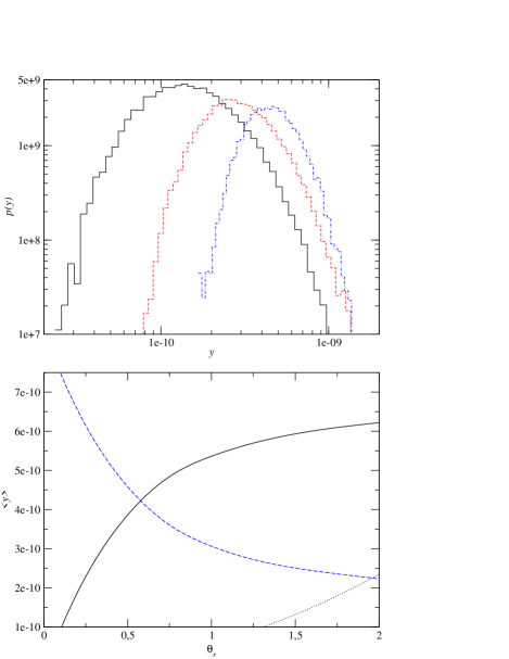
Figure 7: Top: Probability density $p(y)$ for different aperture radii: $\theta_{\rm r}=0.25^{\circ}$ (solid), $\theta_{\rm r}=0.5^{\circ}$ (dashed) and $\theta_{\rm r}=1.0^{\circ}$ (dashed-dotted). — Bottom: Dependence of the average y-parameter on the aperture radius $\theta_{\rm r}$ in degrees: for the beam spectral distortion (solid) and for the y-parameter resulting from the dispersion of the beam RJ temperatures in different directions on the sky relative to $T_{0}$ (dashed). Also shown is the maximal beam spectral distortion arising due to the dipole, $y_{\rm r,max}$ (dotted), according to equation (53).

In Fig. 7 the probability density $p(y)$ for a given aperture is shown. It is defined such that $p(y)\,dy$ gives the probability to find a value of the y-parameter in a random direction on the sky between $y$ and $y+dy$ for a given beam radius. As expected, the average value $\left<y\right>$ increases with aperture radius, while the width of $p(y)$ decreases. For $\theta_{\rm r}\gtrsim 1$ the average beam y-parameter varies only slowly. In the limit of a whole sky measurement, the y-parameter converges to $y_{\rm h}=8.33\cdot 10^{-10}$, which corresponds to the whole sky rms dispersion $\Delta T\sim 111\,\mu$K of the used realization of the CMB sky. For $\theta_{\rm r}\lesssim 1$ the beam y-parameter falls off very fast. As Fig. 7 suggests, for $\theta_{\rm r}\lesssim 2-5^{\circ}$ the distortions arising due to the dipole are negligible in comparison to the distortions arising due to higher multipoles.

Figure 7 also shows the y-parameter resulting from the dispersion of the beam RJ temperatures in different directions on the sky relative to $T_{0}$. It drops with increasing beam radius, because the average beam RJ temperature becomes closer to $T_{0}$ for bigger beam radius. Looking at the sum of the beam distortion and the distortion due to the dispersion of the beam RJ temperatures shows that the averaged whole sky distortion is independent of the angular resolution.

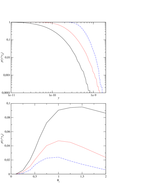
Figure 8: Top: Cumulative probability $p(y\geq y_{0})$ for different aperture radii $\theta_{\rm r}=0.1^{\circ}$ (solid), $\theta_{\rm r}=0.25^{\circ}$ (dashed) and $\theta_{\rm r}=1.0^{\circ}$ (dashed-dotted). – Bottom: Dependence of the cumulative probability $p(y\geq y_{0})$ on the aperture $\theta_{\rm r}$ for $y_{0}=8\cdot 10^{-10}$ (solid), $y_{0}=9\cdot 10^{-10}$ (dashed) and $y_{0}=10^{-9}$ (dashed-dotted).

In Fig. 8 the cumulative probability for finding a spectral distortion with $y\geq y_{0}$ is shown for different apertures. Fixing the value $y_{0}$, there is a maximum probability of $2.4\%$ to measure $y\geq 10^{-9}$ for an aperture radius $\theta_{\rm r}\sim 1^{\circ}$ during the mapping or scanning of extended regions of the sky. This correspond to $\sim 500$ sources on the whole sky. In Fig. 9 the dependence of the number of sources with $y$ above $y_{0}$ for a given radius $\theta_{\rm r}$ is illustrated. It peaks around $\theta_{\rm r}\sim 0.5$ degree, corresponding to the first acoustic peak. We should mention that the maxima of the y-distortion do not coincide with the maxima of $\Delta T/T$, but that they both should have similar statistical properties. We expect that the maxima of the y-parameter are there, where the derivatives of the averaged temperature field are large.

Figure 9: Number of regions on the sky with $y\geq y_{0}$ for different aperture radii $\theta_{\rm r}$ in degree: for $y_{0}=8\cdot 10^{-10}$ (solid), $y_{0}=9\cdot 10^{-10}$ (dashed) and $y_{0}=10^{-9}$ (dashed-dotted).

The motion induced CMB octopole

In section 5 we discussed spectral distortions due to the motion of the solar system relative to the CMB restframe up to second order in $\beta_{\rm d}$. On the level of $y\sim 10^{-10}-10^{-9}$ third order corrections $\propto\beta_{\rm d}^{3}$ should also start to contribute. In this order of $\beta_{\rm d}$ not only the motion induced dipole and quadrupole lead to spectral distortions but also terms connected to the products of the intrinsic dipole and quadrupole with the motion induced dipole and quadrupole. Here we now only discuss the motion induced CMB third order terms.

Expanding (42a) up to third order in $\beta_{\rm d}$ and calculating the beam averaged RJ temperature for the top-hat beam using (47) leads to

$$\bar{T}_{\rm r,oct}=\bar{T}_{\rm r}+T_{0}\,\beta_{\rm d}^{3}\,\zeta_{+}\,\left[\frac{1}{10}\,\mu_{0}\right.\\ \left.+\left(1-5\,\zeta_{+}\,\zeta_{-}\right)\mu_{0}\!\left(\mu_{0}^{2}-\frac{3}{5}\right)\right]\,,$$ (64)

where $\bar{T}_{\rm r}$ is given by (50). In addition to the motion induced octopole in third order of $\beta_{\rm d}$ there also is a correction to the CMB dipole. Now we can also recalculate the second beam moment leading to a y-parameter of

$$y_{\rm r,oct}=y_{\rm d}\,\beta_{\rm d}\cdot\left[\mu_{0}\left(1+\frac{7}{5}\,\mu_{\rm r}\right)-6\,\mu_{0}\!\left(\mu_{0}^{2}-\frac{3}{5}\right)\right]\zeta_{+}\,\zeta_{-}\,,$$ (65)

for the third order in $\beta_{\rm d}$. The total motion induced y-parameter is then given by the sum $y=y_{\rm r}+y_{\rm r,oct}$, where $y_{\rm r}$ is given by (52). As before in the limit $\theta_{\rm r}\rightarrow 0$ the y-parameter $y_{\rm r,oct}$ vanishes. It has a dipole and octopole angular dependence and reaches a maximal value of $y_{\rm r,oct}\sim 9.6\cdot 10^{-11}$ in the $\mu_{0},\theta_{\rm r}$-plane. Therefore one may completely neglect the contribution of the second beam moment to the y-parameter. If we consider the third beam moment we find

$$\left<\delta^{3}\right>_{\rm r}=6\,y_{\rm d}\,\beta_{\rm d}\cdot\left[-\frac{2}{5}\,\mu_{0}+\mu_{0}\!\left(\mu_{0}^{2}-\frac{3}{5}\right)\right]\zeta_{+}\,\zeta_{-}^{2}\,.$$ (66)

It reaches a maximal value of $\left<\delta^{3}\right>_{\rm r}/6\sim 1.8\cdot 10^{-11}$. Due the strong dependence on $\theta_{\rm r}$ we may therefore also neglect any contribution of the third beam moment.

7 Spectral distortions induced in differential measurements of the CMB sky

In Sect. 5 we discussed the spectral distortion arising due to the CMB dipole inside a single circular beam in comparison to a reference blackbody with temperature $T_{0}$. In this chapter we address the spectral distortion arising in differential measurements of the CMB fluctuations, where two beam intensities $I_{1}$ and $I_{2}$ are directly compared with each other and the intensity difference $\Delta I=I_{2}-I_{1}$ is measured. Since in Sect. 6 we have shown that y-distortion arising due to higher multipoles have corresponding y-parameters $y\leq 10^{-9}$, here we are only taking distortions arising due to the CMB dipole into account. If we assume that the both beams are circular and have the same radius $\theta_{\rm r}$ (see Fig. 10), we may define the beam RJ temperatures as $\bar{T}_{\rm r,1}$ and $\bar{T}_{\rm r,2}$, where $\bar{T}_{\rm r,\it i}$ of each beam is given by equation (50).

Figure 10: Illustration of a differential observing strategy: The maximum of the dipole lies in the direction of the $z$-axis. Both observed patches have the same radius $\theta_{\rm r}$ and the observed intensity difference is $\Delta I=I_{2}-I_{1}$.

Now, defining the reference blackbody $I_{\ast}=B_{\nu}(T_{\ast})$ with temperature $T_{\rm ref}=T_{\ast}$ using equations (7) and (29) we find for the inferred temperature difference at frequency ${\hat{x}}_{\ast}=h\nu/k\,T_{\rm ref}$

$$\frac{\Delta T({\hat{x}}_{\ast})}{T_{\ast}} =\Delta_{\rm r,12}+y_{\rm r,12}\cdot g_{y}({\hat{x}}_{\ast})\,,$$ (67)

where we have introduced the abbreviations

$$\Delta_{\rm r,12} =\frac{\bar{T}_{\rm r,2}-\bar{T}_{\rm r,1}}{T_{\ast}}$$ (68a)

$$y_{\rm r,12} =y_{\rm b,r}+{y_{\rm ref}}$$ (68b)

$${y_{\rm ref}} =\frac{\bar{T}_{\rm r,2}-\bar{T}_{\rm r,1}}{\bar{T}_{\rm r,1}+\bar{T}_{\rm r,2}}\cdot\frac{\bar{T}_{\rm r,1}+\bar{T}_{\rm r,2}-2\,T_{\ast}}{T_{\ast}}\,.$$ (68c)

Using equation (52), the difference of the beam y-parameters $y_{\rm b,r}=y_{\rm r}(\mu_{2})-y_{\rm r}(\mu_{1})$ can be written as

$$y_{\rm b,r} =-3\,y_{\rm d}\,\Delta\mu\,[2\,\mu_{1}+\Delta\mu]\,\zeta_{+}\,\zeta_{-}\,,$$ (69)

where $\mu_{i}=\cos\theta_{i}$, $\Delta\mu=\mu_{2}-\mu_{1}$ and $\theta_{i}$ is the angle between the dipole axis and the beam $i$. Here it is important to note, that in the case $\Delta\mu=2$, i.e. when we are comparing the maximum and minimum of the CMB dipole $y_{\rm b,r}\equiv 0$, since both beams have the same shape and size. In this case we are directly dealing with the difference of two blackbodies with temperatures $\bar{T}_{\rm r,\it i}$ and we may apply the results obtained earlier in Sect. 4.

Now one can write for the relative temperature difference of the two beams at two frequency ${\hat{x}}_{\ast,1}$ and ${\hat{x}}_{\ast,2}$, with ${\hat{x}}_{\ast,2}>{\hat{x}}_{\ast,1}$ and ${\hat{x}}_{\ast,i}=h\nu_{i}/k\,T_{\ast}$ as

$$\Delta\Delta =\frac{\Delta T({\hat{x}}_{\ast,2})-\Delta T({\hat{x}}_{\ast,1})}{T_{\ast}}$$

$$=y_{\rm r,12}\cdot[g_{y}({\hat{x}}_{\ast,2})-g_{y}({\hat{x}}_{\ast,1})]\,.$$ (70)

If we assume that ${\hat{x}}_{\ast,1}\ll 1$, i.e. for a measurement in the RJ region of the CMB spectrum, then we can approximate $g_{y}({\hat{x}}_{\ast,1})\approx{\hat{x}}_{\ast,1}^{2}/6$. For estimates we will assume that $g_{y}({\hat{x}}_{\ast,1})=0$.

On the CMB sky the most natural choices for the reference temperature is the full sky mean temperature $T_{0}$ and the temperature of the maximum or the minimum of the CMB dipole anisotropy, whereas the last two are equivalent. Below we now discuss the dependence of the inferred y-parameter on the angle between the beams for these two choices of the reference temperature. In the limit $\theta_{\rm r}\rightarrow 0$ we can apply the results obtained in Sect. 4.2 for the difference of two blackbodies.

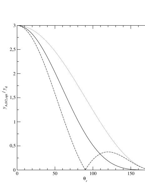
Figure 11: Dependence of the y-parameter in units of $y_{\rm d}=2.6\cdot 10^{-7}$ on the beam radius $\theta_{\rm r}$ in degree for differential measurements: $y_{\mathcal{A},0,\rm opt}$ as given by equation (73) (dashed/left ordinate), $y_{\mathcal{A},1,\rm opt}$ as given by equation (76) (solid/right ordinate) and $y_{\mathcal{A},2,\rm opt}$ as given by equation (77) (dotted/left ordinate) .

Case $T_{\ast}=T_{0}$

In this case, making use of equation (50) and (68c) one may find

$$y_{\rm ref,0} =3\,y_{\rm d}\,\Delta\mu\,[2\,\mu_{1}+\Delta\mu]\,\zeta_{+}^{2}+\mathcal{O}(\beta_{\rm d}^{3})\,.$$ (71)

Using the beam y-parameter $y_{\rm b,r}$ as given in equation (69) we find for the corresponding total inferred y-parameter

$$y_{\rm\mathcal{A},0}=3\,{y_{\rm d}}\left|\mu_{\rm r}\,\zeta_{+}\,\Delta\mu\cdot[2\,\mu_{1}+\Delta\mu]\right|+\mathcal{O}(\beta_{\rm d}^{3})\,.$$ (72)

The largest values of the y-parameter in the $\mu_{1},\Delta\mu$-plane are obtained for the combinations $(\mu_{1},\Delta\mu)=(0,1)$, $(0,-1)$, $(1,-1)$, $(-1,1)$. In these optimal cases it follows

$$y_{\mathcal{A},0,\rm opt}=3\,{y_{\rm d}}\,\zeta_{+}\left|\mu_{\rm r}\right|+\mathcal{O}(\beta_{\rm d}^{3})\,.$$ (73)

The dependence of $y_{\mathcal{A},0,\rm opt}$ on the radius of the beam is shown in Fig. 11. The distortion does not vanish for high angular resolution ($\theta_{\rm r}\rightarrow 0$) and the maximum is 3 times bigger than ${y_{\rm d}}$. The corresponding absolute temperature difference in some of the Planck frequency channels are given in Table LABEL:tab:one. For $\theta_{\rm r}=\pi/2$ the y-distortion vanishes.

Let us note here, that in the case $\Delta\mu=2$, i.e. when we are directly comparing the maximum and the minimum of the CMB dipole, the spectral distortion vanishes. This can be understood as follows: As was argued in Sect. 3.2, if the chosen reference temperature is equal to $T_{y=0}$ as given by equation (34) the total y-parameter is zero. For $\mu_{1}=-1$ and $\mu_{2}=1$ the beam moments $\left<\delta_{i}^{2}\right>_{\rm r,\it i}$ are both equal and therefore do not contribute to the total inferred y-parameter (68b). In this case we obtain $T_{y=0}=T_{\mathrm{RJ}}=(\bar{T}_{\rm r,1}+\bar{T}_{\rm r,2})/2=T_{0}+\mathcal{O}(\beta_{\rm d}^{2})$. Therefore, consistent in second order of $\beta_{\rm d}$ the total inferred y-parameter vanishes. This conclusion can also be directly drawn from equation (36).

Case $T_{\ast}=\bar{T}_{\rm r,1}$

In this case, again making use of equation (50) and (68c) one may find

$$y_{\rm ref,1} =3\,y_{\rm d}\,\Delta\mu^{2}\,\zeta_{+}^{2}+\mathcal{O}(\beta_{\rm d}^{3})\,.$$ (74)

Now using equation (69) we may write the total inferred y-parameter as

$$y_{\rm\mathcal{A},1}=3\,{y_{\rm d}}\zeta_{+}\,\left|\Delta\mu\cdot[\mu_{\rm r}\,\mu_{2}-\mu_{1}]\right|+\mathcal{O}(\beta_{\rm d}^{3})\,.$$ (75)

The largest values of the y-parameter in the $\mu_{1},\Delta\mu$-plane are obtained for the combinations $(\mu_{1},\Delta\mu)=(1,2)$ and $(-1,-2)$. In these optimal cases the y-parameter is

$$y_{\mathcal{A},1,\rm opt}=12\,{y_{\rm d}}\,\zeta^{2}_{+}+\mathcal{O}(\beta_{\rm d}^{3})\,.$$ (76)

For high resolution ($\zeta_{+}\rightarrow 1$) we can obtain $y_{\mathcal{A},1,\rm opt}$ directly as the difference of two Planck spectra with temperature corresponding to the maximum $T_{2}$ and the minimum $T_{1}$ of the dipole using (41b) with $T_{\rm ref}=T_{1}$. In this case we directly get $\frac{1}{2}\,[(T_{2}-T_{1})/T_{1}]^{2}=2\,\beta_{\rm d}^{2}=12\,y_{\rm d}$. As will be discussed later this way of comparing the maximum and minimum of the CMB dipole should open a way to cross calibrate the frequency channels in future experiments with full sky coverage to very high precision (Sect. 8).

The dependence of $y_{\mathcal{A},1,\rm opt}$ on the beam radius is shown in Fig. 6. As in the previous case, the y-distortion does not vanish for high resolution ($\theta_{\rm r}\rightarrow 0$) and in the maximum it is even 12 times bigger than ${y_{\rm d}}$, corresponding to $y_{\rm opt}=3.1\cdot 10^{-6}$. This is only $\sim 5$ times below the current upper limit on the mean y-parameter given by Cobe/Firas. The corresponding absolute temperature difference in some of the Planck frequency channels are given in Table LABEL:tab:one.

Another case may be interesting for CMB missions with partial sky coverage, but which have access to the maximum or the minimum of the dipole ($\mu_{1}=\pm 1$) and a region in the directions perpendicular to the dipole axis ($\mu_{2}=0$): Using (75) with $(\mu_{1},\Delta\mu)=(\pm 1,0)$ one obtains

$$y_{\mathcal{A},2,\rm opt}=3\,{y_{\rm d}}\,\zeta_{+}+\mathcal{O}(\beta_{\rm d}^{3})\,.$$ (77)

In this case the amplitude is comparable to $y_{\rm\mathcal{A},0}$, but the dependence on the beam radius $\theta_{\rm r}$ is much weaker (see Fig. 6).

8 Cross Calibration of frequency channels

The cross calibration of the different frequency channels of CMB experiments is crucial for the detection of any frequency dependent signal. As has been mentioned earlier usually the dipole and its annual modulation due to the motion of the earth around the sun is used for calibration issues. The amplitude of the dipole is known with a precision of $\sim 0.3\%$ on a level of $\Delta T\sim\,$mK. But the sensitivities of future experiments will be significantly higher than previous missions and request a possibility for cross calibration down to the level of tens of nK.

In this Sect. we now discuss two alternative ways to cross calibrate the frequency channels of future CMB experiments. Most importantly we show that making use of the superposition of blackbodies and the spectral distortions induced by the CMB dipole should open a way to cross calibrate down to the level necessary to detect signals from the dark ages as proposed by Basu et al. (2003).

8.1 Calibration using clusters of galaxies

It is obvious, that brightest relaxed clusters of galaxies on the sky open additional way to cross calibrate the different frequency channels of future CMB experiments like Planck and ground based experiments like Act. The CMB signal of the majority of rich clusters has very distinct y-type spectrum due to the thermal SZE. Multifrequency measurements allow to determine their y-parameters and thereby open a way to use them as sources for cross calibration. This cross calibration will then enable us to detect the effects of relativistic correction for very hot clusters and thereby to measure the temperatures of clusters independent of X-ray observations.

Clusters such as Coma, where existing X-ray data provide excellent measurements of the electron densities and temperatures inside the cluster and where we know the contamination of the CMB brightness by radiosources and the dust in galaxies very well, even may be used for absolute calibration of CMB experiments. For the Coma cluster today X-ray data allows us to predict the CMB surface brightness with precision of the order of a few percent.

Due to the redshift independence of the SZ signal, distant clusters have similar surface brightness but much smaller angular diameters. Therefore they are good sources for calibration issues for experiments covering only limited parts of the sky and having high angular resolution like Act (for example Act is planing to investigate 200 square degree of the sky (Kosowsky, 2003)).

One disadvantage of clusters for cross calibration purposes is that they are too bright: Typically clusters have y-parameter of the order of $\sim 10^{-5}-10^{-4}$ and therefore are only a few times weaker than the temperature signal of the CMB dipole ($\sim 3\,$mK). In comparison to the level of calibration and cross calibration achieved directly using the dipole this is not much of an improvement.

In addition planets or galactic and extragalactic radiosources might serve for cross calibration purposes, if we know their spectral features with very high precision. Quasars and Active Galactic Nuclei are not good candidates for this issue, since they are highly variable in the spectral band of interest.

8.2 Cross calibration using the superposition of blackbodies

All the sources mentioned in Sect. 8.1 do not allow cross calibration down to the level of the sensitivity of future CMB experiments and do not enable us to detect signals from the dark ages as predicted by Basu et al. (2003). Therefore here we want to discuss a method to cross calibrate the frequency channel using the spectral distortions induced by the CMB dipole (see Sect. 5). These spectral distortions can be predicted with very high accuracy on a level of $\sim\mu$K. This is $\sim 1000$ times lower than the dipole signal and should therefore allow cross calibration to a very high precision.

Every CMB experiment is measuring the fluctuations of the CMB intensity on the sky. Due to the nature of the physical processes producing these fluctuations in each point they are related to the fluctuations of the radiation temperature. In a map making procedure the measured fluctuations in the intensity are translated into the fluctuations in the radiation temperature. Usually the aim of any map making procedure is to reduce statistic and systematic error in order to obtain a clean signal from these CMB temperature fluctuations. As has been discussed in Sects. 3 the superposition of blackbodies with slightly different temperature in second order induces y-distortions in the inferred temperature differences. The amplitude of these distortions depends on the temperature difference and the chosen reference temperature. In Sects. 5 and 7 it has been shown that due to the two basic observing strategies, absolute and differential measurements, the dipole can induce y-distortions with y-parameters up to $y\sim 10^{-6}$. It was also shown in Sect. 6 that contributions from higher multipoles are much smaller ($y\sim 10^{-11}-10^{-9}$).

The y-distortions induced by the dipole can contaminate the maps produced in the map making procedure on a level higher than the sensitivity of the experiment. Therefore it is important to chose the map making procedure such that spectral distortions are minimized. The discussion in Sects. 4 has shown, that for this purpose in absolute measurements of the CMB sky it is the best to choose the temperature of the reference blackbody close to the beam RJ temperature. This implies that for CMB experiment the best choice for the temperature of the internal calibrator is the full sky mean temperature $T_{0}$. In order to minimize the spectral distortions arising due to the superposition of blackbodies in differential measurements the best choice for the reference temperature used to relate the intensity difference maps to the temperature difference maps is the RJ temperature of the combined temperature distribution of both beams. This optimal reference temperature will be time dependent due to the various scanning strategies and orientations of the spinning axis relative to the dipole during observations.

The purpose of this Sect. is not to discuss details about map making procedures but to show, that there are ways to manipulate these CMB maps in order to make the spectral distortions arising due to the superposition of blackbodies become useful for cross calibration purposes. As the discussion in Sect. 4 has shown, for this issue it is better to move $T_{\rm ref}$ as far as possible away from $T_{0}$. The optimal choice of $T_{\rm ref}$ depends on the sensitivity of the experiment and on the observing strategy: For absolute measurements $T_{\rm ref}$ should be as close as possible to $T_{0}$ in order to minimize the induced y-distortions but on the other hand it should be chosen such that the induced y-distortion due to the CMB dipole is still measurable within the sensitivity of the experiment. But in principle there is no strong constrain, since the induced y-distortions can again eliminated afterwards. For differential measurements it is possible to chose the optimal reference temperature for calibration issues independent of the best map making reference temperature, but here it is important to compare regions on the sky with maximal temperature difference, i.e. with maximal angular separation in the observed field. Below we now separately discuss CMB experiments using differential measurements with full and partial sky coverage in more detail.

Full sky CMB surveys

For full sky missions like Planck the regions with maximal temperature difference are located around the extrema of the CMB dipole. Using equation (75) we see that they correspond to $\Delta\mu=2$ and the resulting maximal spectral distortion is characterized by $y_{\rm opt}=12\,y_{\rm d}=3.1\cdot 10^{-6}$, if we set $T_{\rm ref}=\bar{T}_{\rm r,1}$ or $T_{\rm ref}=\bar{T}_{\rm r,2}$, i.e. to the maximum or minimum of the temperature on the CMB sky arising due to the dipole.

Table 1: y-distortion: $\Delta T=T_{\rm ref}\cdot y$ in $\mu$K for $y$ as given in the left column in some of the Planck spectral channels. Here $y_{\rm d}=2.6\cdot 10^{-7}$, $y_{\rm opt,0}=3\,{y_{\rm d}}$ and $y_{\rm opt}=12\,{y_{\rm d}}$.

	Center of channels [GHz]
$\nu_{\rm c}$	30	44	70	100	143	217	353
$y_{\rm d}$	0.03	0.07	0.17	0.34	0.67	1.39	2.97
$y_{\rm opt,0}$	0.10	0.21	0.52	1.03	2.01	4.18	8.90
$y_{\rm opt}$	0.39	0.83	2.07	4.13	8.05	16.71	35.56

One attractive procedure to compare the maximum and minimum of the CMB dipole is to take the CMB intensity maps of each spectral channel and to calculate the difference between each map and the map obtained by remapping the value of the intensity $I(\mbox{\boldmath${n}$\unboldmath})$ at position ${n}$ to the value $I(-\mbox{\boldmath${n}$\unboldmath})$ at position $-\mbox{\boldmath${n}$\unboldmath}$, i.e rotating the initial map by $180$ degrees around any axis, which is perpendicular to the CMB dipole axis and is crossing the origin or equivalently setting $\mu_{2}=-\mu_{1}$ in equation (67).

Afterwards these artificial intensity maps for each spectral channel are converted into temperature maps using equation (7) and setting the reference temperature at each point to $T_{\ast}(\mbox{\boldmath${n}$\unboldmath})=\bar{T}_{\rm r,1}(\mbox{\boldmath${n}$\unboldmath})$ of the intrinsic map. Neglecting the contributions from intrinsic multipoles with $l\geq 2$, the difference map in some frequency channel ${\hat{x}}_{\ast}=h\nu/k\,\bar{T}_{\rm r,1}$ will be given by

$$\frac{\Delta T({\hat{x}}_{\ast},\@vec{n})}{\bar{T}_{\rm r,1}(\@vec{n})}=-2\,\beta_{\rm d}\,\zeta_{+}\,\mu+2\,\beta_{\rm d}^{2}\,\zeta_{+}^{2}\,\mu^{2}\\ +12\,y_{\rm d}\,\zeta^{2}_{+}\,\mu^{2}\cdot g_{y}({\hat{x}}_{\ast})\,,$$ (78)

where we used the definition (5) for $g_{y}({\hat{x}})$. This shows, that the artificial maps will contain a frequency independent temperature dipole component with twice the initial dipole amplitude and a monopole and quadrupole y-distortion resulting from the second term in (78). The maxima of the spectral distortion will coincide with the extrema of the CMB dipole.

Now, using the artificial map of the lowest frequency channel as a reference and taking the differences between this reference map and the artificial maps in higher spectral channels we can eliminate the frequency independent term corresponding to twice the dipole in equation (78). This then opens a way to cross calibrate all the channels to very high precision, since the quadrupole component in these artificial maps will be larger in higher spectral channels, following the behavior of $g_{y}$ with ${\hat{x}}$.

The signal will include both statistical and systematic errors for the average temperature of the sky and the dipole amplitude $\beta_{\rm d}$. All uncertainties are mainly influencing the frequency independent dipole term but for the frequency dependent monopole and quadrupole they will become important only in next order:

$$\bar{T}_{1}\cdot\beta_{\rm d}^{2} =\bar{T}_{1,0}\,\beta_{\rm d,0}^{2}\,(1\pm\Delta_{T})\cdot(1\pm\Delta_{\beta})^{2}$$

$$=\bar{T}_{1,0}\,\beta_{\rm d,0}^{2}\,[1\pm 2\,\Delta_{\beta}\pm\Delta_{T}]+\mathcal{O}(\Delta_{\beta}\cdot\Delta_{T})\,,$$ (79)

where $\bar{T}_{1,0}$ is the correct value of the temperature at a given point on the sky, $\beta_{\rm d,0}$ is the correct dipole amplitude and $\Delta_{T}$ and $\Delta_{\beta}$ are their corresponding relative uncertainties. This implies that all the corrections to the frequency dependent terms are at least 1000 times smaller than the signal we are discussing here. On this level correction due to higher order moments might become important, but their contributions will be less than 1%. This means that y-distortion on a level of $10\,\mu$K can be predicted with $\sim 100\,$nK precision.

Let us note here, that applying the procedure as described above we are adding signals which have statistically independent noise. Therefore the statistical noise of the artificial maps should be a factor of $2/\sqrt{2}=\sqrt{2}$ stronger than the initial maps. On the other hand we are increasing the amplitude of the y-distortion quadrupole by a factor of $12$, resulting in strong gain.

The maxima of the quadrupole component in the artificial maps will be rather broad and correspond to thousands of square degrees on the sky, allowing to average the signal and thereby increasing the sensitivity. For circular beam average formula (78) will be applicable. The statistical sensitivity of the Planck experiment will permit to find these spectral distortions in the artificial maps down to the level which is necessary to detect the effects of reionization as discussed by Basu et al. (2003). Applying the above procedure to the $33\,$GHz and $93\,$GHz frequency channels of Wmap will lead to a maximal temperature difference of $\Delta T=3.6\,\mu$K, whereas the maximal difference will be $\Delta T=35.6\,\mu$K for the $353\,$GHz channel of Planck (see Table LABEL:tab:one). Nevertheless, even in the case of Wmap the very high precision of the experiment might permit the detection of this quadrupole and thereby open the way to cross calibrate its different spectral channels.

For Cobe/Firas the proposed method permits to check the precision of the internal calibration. The internal calibrator was measured and tested with some finite precision and there is the possibility that the internal calibration may be better than the precision at which it was tested. The proposed method has distinct spectral and angular properties, making it possible to improve the cross calibration of the spectral channels and possibly this will open a way to further improve the great results this experiment already gave us.

CMB surveys with partial sky coverage

Surveys with partial sky coverage may not simultaneously have access to regions around the maximum and the minimum of the dipole. Therefore here one should choose two regions in the accessible field of view such that the mean temperature difference between these regions is as large a possible. The dependence of the signal on the separation angle has been discussed in detail in Sect. 7.

Before cross calibration all the bright sources detected such as bright clusters of galaxies and point sources inside the chosen areas should be extracted. Typically the expected amount of SZ sources will be of the order of a few tens per square degrees with corresponding angular extensions less than $1^{\prime}$ (see Carlstrom & Holder, 2002; Rubiño-Martín & Sunyaev, 2003). Afterwards the difference of the signals in the two patches can be taken and compared to the signals in the other spectral channels.

For example choosing one area centered on the minimum or maximum of the CMB dipole as a reference ($T_{\ast}=\bar{T}_{\rm r,1}$) and choosing the second area in the ring perpendicular to the dipole axis the maximal y-parameter is $y=3\,y_{\rm d}\,\zeta_{+}=7.7\cdot 10^{-7}\,\zeta_{+}$ (cf. equation (77)). If we instead set $T_{\ast}=T_{0}$ we obtain the same maximal y-parameter but a stronger dependence on the beam radius or size of the regions we average (cf. equation (73)). This small example shows that for any experiment with partial sky coverage a separate analysis of the optimal choice of the reference temperature and the regions on the sky has to be done.

9 Other sources of spectral distortions

Injection of energy into the CMB prior to recombination leads to spectral distortions of the background radiation. Given the Wmap best fit parameters, before redshift $z_{\rm th}\sim 2\cdot 10^{6}$ all distortions are efficiently wiped out, whereas energy injection in the redshift range $z_{\rm th}>z>z_{\mu}$, with $z_{\mu}\sim 1.4\cdot 10^{5}$, leads to a $\mu$-distortion and injection in the range $z_{\mu}>z>z_{\rm rec}$ to a y-distortion, with $z_{\rm rec}\sim 1090$ (Sunyaev & Zeldovich, 1970b; Illarionov & Sunyaev, 1975; Burigana, Danese & Zotti, 1991; Hu & Silk, 1993).

As was shown by Silk (1968) photon diffusion and thermal viscosity lead to the dissipation of small scale density perturbations before recombination. This damping of acoustic waves will contribute to a $\mu$- and y-distortion because it was leading to (i) energy release (Sunyaev & Zeldovich, 1970b; Daly, 1991; Hu, Scott & Silk, 1994a) and (ii) mixing of photons from regions having different temperatures (Zeldovich, Illarionov & Sunyaev, 1972).

Now, the Wmap data implies that the initial spectrum of perturbations is close to a scale-invariant Harrison-Zeldovich spectrum with spectral index $n=1.03\pm 0.04$ (Bennett et al., 2003). Different estimates for the spectral distortions arising from the dissipation of acoustic waves in the early universe give a chemical potential of the order of $\mu_{\rm dis}\sim 2\cdot 10^{-7}$ and y-distortions with $y_{\rm dis}\sim 10^{-7}$ (Daly, 1991; Hu, Scott & Silk, 1994a).

Another contribution to the y-distortion arises from the epoch of reionization (Zeldovich & Sunyaev, 1969; Hu, Scott & Silk, 1994b) and from the sum of the SZE of clusters of galaxies (Markevitch et al, 1991). The Wmap results for the TE power spectrum point towards an early reionization of the universe with corresponding optical depth $\tau_{\rm re}=0.17\pm 0.04$ (Kogut et al, 2003; Spergel et al, 2003). Here two main effects are important: (i) The photoionized gas typically has temperatures $T$ of the order of $\sim 10^{4}\,$K. Therefore the diffuse gas after reionization will produce a y-distortion in the CMB spectrum with

$$y_{\rm re}\sim\int\frac{k\,T}{m_{\rm e}\,c^{2}}\,{\,\rm d}\tau\sim 3\cdot 10^{-7}\;\frac{\tau_{\rm re}}{0.17}\;\frac{T}{10^{4}\,\text{K}}\,.$$

(ii) The motion of the matter induces a y-distortion on the whole sky due to the second order Doppler effect, with corresponding y-parameter (Hu, Scott & Silk, 1994b), $y_{v}=\frac{1}{3}\int\sigma_{\rm T}\,n_{\rm e}\,c\left<v^{2}\right>{\,\rm d}t$, where $\left<v^{2}\right>$ is the velocity dispersion over the whole sky in units of the speed of light. For a CDM model it is of the order of

$$\qquad\quad y_{v}\sim 2\cdot 10^{-8}\left(\left[\frac{z_{\rm re}}{10}\right]^{1/2}-1\right)\frac{\left<v^{2}\right>}{10^{-5}}\,\frac{\Omega_{\rm b}h^{2}}{0.0224}\,.$$

Since the reionization optical depth is very small, this is one order of magnitude smaller than $y_{\rm re}$. If secondary ionization was patchy this will in addition lead to angular fluctuations (Santos et al., 2003).

All the effects mentioned in this section lead to y-distortions with corresponding y-parameter in the range $y\sim 10^{-8}-10^{-7}$. As has been shown in Sects. 5 and 7 the y-distortions arising due to the CMB dipole are of the same order. For example the CMB dipole induces a full sky y-distortion with ${y_{\rm d}}=2.6\cdot 10^{-7}$. Therefore, to measure any of the effects discussed above it is necessary to take spectral distortions associated with the CMB dipole into account. But since the angular distribution and the amplitude of these distortions can be accurately predicted they can be easily extracted. As has been shown in Sect. 6 spectral distortions arising from higher multipoles typically have $y\sim 10^{-11}-10^{-9}$ and therefore do not play an important role in this context. But even for these distortions the locations and amplitudes can be accurately predicted with measured CMB maps and therefore offer the possibility to eliminate these distortions from the maps.

10 Conclusion

We have discussed in detail the spectral distortions arising due to the superposition of blackbodies with different temperatures in the limit of small temperature fluctuations. The superposition leads to y-distortion with y-parameter $y_{\rm S}=\left<\delta^{2}\right>/2$, where $\left<\delta^{2}\right>$ denotes the second moment of the temperature distribution function, if the difference in temperatures in less than a few percent of the mean RJ temperature. We have shown that in this limit even comparing to pure blackbodies leads to a y-distortion.

The results of this derivation where then applied to measurements of the CMB temperature anisotropies with finite angular resolution and in particular to the CMB dipole and its associated spectral distortions, but in principle the method developed here can be applied whenever one is dealing with the superposition of blackbodies with similar temperatures. We have shown, that taking the difference of the CMB intensities in the direction of the maximum and the minimum of the CMB dipole leads to a y-distortion with y-parameter $y_{\rm opt}=3.1\cdot 10^{-6}$. This value is 12 times higher than the y-type monopole, $y_{\rm d}=2.6\cdot 10^{-7}$. Since the amplitude of this distortion can be calculated with the same precision as the CMB dipole, i.e. $0.3\%$ today (Fixsen & Mather, 2002), it opens a way to cross calibrate the different frequency channels of CMB experiment down to the level of a few tens of nK ( for more details see Sect. 8).

We discussed another possibility to check the zero levels of different frequency channels by observing the difference of the brightness in the direction of the dipole maximum and in the direction perpendicular to the dipole axis: The dipole induced spectral distortion in this case is 4 times weaker than for the difference of the maximum and minimum and corresponds to $y\sim 7.7\cdot 10^{-7}$. Nevertheless, it is still 3 times stronger than the dipole induced whole sky y-distortion with y-parameter $y_{\rm d}$.

The value of $y_{\rm opt}$ is only 5 times lower than the upper limit on the whole sky y-parameter obtained by the Cobe/Firas experiment Fixsen & Mather (2002) and is orders of magnitudes above the sensitivity of Planck and Cmbpol in each of their spectral channels. Therefore this signal might become useful for both cross calibration and even absolute calibration of different frequency channels of these experiments to very high precision, in order to permit detection of the small signals of reionization as for example discussed by Basu et al. (2003), and to study frequency dependent foregrounds with much higher sensitivity. We should emphasize, that on this level we are only dealing with the distortions arising from the CMB dipole as a result of the comparison of Planck spectra with different temperatures close to the maximum and minimum of the CMB dipole, i.e. due to the superposition of blackbodies. The distortions are introduced due to the processing of the data and become most important in the high frequency channels.

Let us stress that the distortions discussed in this work have both well known spectral and angular dependence and that they are connected with the much stronger signal of the CMB dipole. The amplitude of the dipole is known to a relative precision $\sim 10^{-3}$ and therefore the induced spectral distortions can be calculated to the same accuracy. Maybe the great properties of the calibration source discussed above might even be detectable in the high frequency channels ($x\gtrsim 10$) of the existing Cobe/Firas data and thereby help to further improve its calibration.

The development of the CMB experimental technology is repeating with 20 years delay the progress that was made in the astronomical observations with X-ray grazing incidence mirrors and CCD detectors. Due to the big efforts of many spacecraft teams, the X-ray background today is resolved to more than 85 % (Rosati et al., 2002). During the next decade, CMB observers will be able to pick up all rich clusters of galaxies and all bright y-distorted features connected with supernovae in the early universe, groups of galaxies and even rising down to patchy reionization in the CMB maps. Deep source counts may permit the separation of their contribution to the y-parameter and in principle might bring us close to the level of the y-distortions mentioned in Sect. 9. As has been argued, on this stage the contributions to the y-parameter arising from the superposition of Planck spectra with different temperatures corresponding to the observed CMB temperature fluctuations will be the easiest to separate. Again, the main contribution will arise from the CMB dipole. On the full sky the corresponding y-parameter will be $y_{\rm d}=2.6\cdot 10^{-7}$. But even the distortions arising from the primordial temperature fluctuations with multipoles $l\geq 2$ can lead to distortions of the order of $y\sim 10^{-9}$ in significant parts of the sky. In the future this type of spectral distortion can be taken into account making it possible to enter the era of high precision CMB spectral measurements.