Calibrating the Galaxy Halo – Black Hole Relation Based on the Clustering of Quasars

Abstract

The observed number counts of quasars may be explained either by long-lived activity within rare massive hosts, or by short-lived activity within smaller, more common hosts. It has been argued that quasar lifetimes may therefore be inferred from their clustering length, which determines the typical mass of the quasar host. Here we point out that the relationship between the mass of the black-hole and the circular velocity of its host dark-matter halo is more fundamental to the determination of the clustering length. In particular, the clustering length observed in the 2dF quasar redshift survey is consistent with the galactic halo – black-hole relation observed in local galaxies, provided that quasars shine at $\sim 10$–$100\%$ of their Eddington luminosity. The slow evolution of the clustering length with redshift inferred in the 2dF quasar survey favors a black-hole mass whose redshift-independent scaling is with halo circular velocity, rather than halo mass. These results are independent from observations of the number counts of bright quasars which may be used to determine the quasar lifetime and its dependence on redshift. We show that if quasar activity results from galaxy mergers, then the number counts of quasars imply an episodic quasar lifetime that is set by the dynamical time of the host galaxy rather than by the Salpeter time. Our results imply that as the redshift increases, the central black-holes comprise a larger fraction of their host galaxy mass and the quasar lifetime gets shorter.

1 Introduction

The Sloan Digital Sky Survey (York et al. 2000) and the 2dF quasar redshift survey (Croom et al. 2001a) have measured redshifts for large samples of quasars, and determined their luminosity function over a wide range of redshifts (Boyle et al. 2000; Fan et al. 2001a,b; Fan et al. 2003). The 2dF survey has also been used to constrain the clustering properties of quasars (Croom et al. 2001b). It has been suggested that quasars have clustering statistics similar to optically selected galaxies in the local universe, with a clustering length $R_{0}\sim 8$Mpc. The large sample size of the 2dF quasars also provided clues about the variation of clustering length with redshift (Croom et al. 2001b) and apparent magnitude (Croom et al. 2002). Quasars appear more clustered at high redshift, although with a relatively mild trend. There is also evidence that more luminous quasars may be more highly clustered.

As pointed out by Martini & Weinberg (2001) and Haiman & Hui (2001), the quasar correlation length determines the typical mass of the dark matter halo in which the quasar resides. One may therefore derive the quasar duty-cycle by comparing the number density of quasars with the density of host dark matter halos. The quasar lifetime then follows from the product of the duty-cycle and the lifetime of the dark-matter halo in between major mergers, although there is a degeneracy between the lifetime and the quasar occupation fraction or beaming. Preliminary results suggested quasar lifetimes of $t_{\rm q}\sim 10^{6}-10^{7}$ years, consistent with the values determined by other methods (see Martini 2003 for a review), including the transverse proximity effect (Jakobsen et al. 2003) and counting arguments relative to the local population of remnant supermassive black holes (SMBHs; see Yu & Tremaine 2002). Kauffmann & Haehnelt (2002) used a detailed semi-analytic model (Kauffmann & Haehnelt 2000) to predict the correlation length of quasars and its evolution with redshift. They found that their model reproduces the correct correlation length as well as its redshift evolution for present-day quasar lifetimes of $t_{\rm q}\sim 10^{7}$ years.

In this work we argue that the correlation length of quasars is fundamentally determined by the relation between the masses of SMBHs and their host galactic halo rather than by the quasar lifetime. We find that the amplitude of the correlation length depends on the product of the SMBH–halo relation and the typical fraction of the Eddington luminosity at which quasars shine. Moreover, we show that the evolution of the correlation length is sensitive to how the SMBH – halo relation evolves with redshift, and therefore to the physics of SMBH formation and quasar evolution.

The paper is organized as follows. In § 2 and § 3 we discuss the calculation of the correlation function of quasars with a particular apparent magnitude $B$, and the different scenarios for the evolution of the SMBH – galaxy halo relation. In § 4 we compare fiducial model correlation functions to the results of the 2dF quasar redshift survey (Croom et al. 2001b,c). We find that the shallow evolution of the correlation length implies that SMBH mass has a redshift-independent scaling with the circular velocity of the host dark matter halo rather than with its mass. The ranges of the normalizations in the SMBH – galaxy halo relation and of the fraction of Eddington allowed by observations of the observed quasar correlation function are explored in § 5. In § 6 we examine the quasar lifetime by requiring that observational constraints from both the correlation and luminosity functions be satisfied simultaneously. Finally, in § 8 we summarize our results and discuss a very simple, physically motivated model that satisfies all constraints with no free parameters. Throughout the paper we adopt the set of cosmological parameters determined by the Wilkinson Microwave Anisotropy Probe (WMAP, Spergel et al. 2003), namely mass density parameters of $\Omega_{m}=0.27$ in matter, $\Omega_{b}=0.044$ in baryons, $\Omega_{\Lambda}=0.73$ in a cosmological constant, and a Hubble constant of $H_{0}=71~{}{\rm km\,s^{-1}\,Mpc^{-1}}$.

2 The Correlation Function of Quasars

The mass correlation function between halos of mass $M_{1}$ and $M_{2}$, separated by a co-moving distance $R$ is (see Scannapieco & Barkana 2003 and references therein)

$$\xi_{\rm m}(M_{1},M_{2},R) = \frac{1}{2\pi^{2}}\int dkk^{2}P(k)$$ (1)

$$\times \frac{\sin(kR)}{kR}W(kR_{1})W(kR_{2}),$$

where

$$R_{1,2}=\left(\frac{3M_{\rm 1,2}}{4\pi\rho_{\rm m}}\right)^{1/3},$$ (2)

$W$ is the window function (top-hat in real space), $P(k)$ the power spectrum and $\rho_{\rm m}$ is the cosmic mass density. The dark-matter halo correlation function for halos of mass $M$ is obtained from the product of the mass correlation function $\xi_{\rm m}(M,M,R)$ and the square of the ratio between the variances of the halo and mass distributions. This ratio, $b$, is defined as the halo bias; its value for a halo mass $M$ may be approximated using the Press-Schechter formalism (Mo & White 1996), modified to include non-spherical collapse (Sheth, Mo & Tormen 2001)

$$b(M,z)=1+\frac{1}{\delta_{\rm c,0}} \left[\nu^{\prime 2}+b\nu^{\prime 2(1-c)}\right.$$ (3)

$$\left.-\frac{\nu^{\prime 2c}/\sqrt{a}}{\nu^{\prime 2c}+b(1-c)(1-c/2)}\right],$$

where $\delta_{\rm c,0}$ ($\approx 1.69$) is the critical overdensity threshold for spherical collapse, $\delta_{\rm c}(z)=\delta_{\rm c,0}/D(z)$, $D(z)$ is the growth factor at redshift $z$, $\sigma$ is the variance on a mass-scale $M$, $\nu\equiv{\delta_{\rm c}^{2}(z)}/{\sigma^{2}(M)}$, $\nu^{\prime}\equiv\sqrt{a}\nu$, $a=0.707$, $b=0.5$ and $c=0.6$. This expression yields an accurate approximation to the halo bias determined from N-body simulations (Sheth, Mo & Tormen 2001).

We need the halo correlation function between halos of different masses. The bias (equation 3) yields the excess probability relative to the mass distribution of finding a halo at any point. We may therefore determine the halo correlation function for halos of mass $M_{1}$ and $M_{2}$ using the product of the biases for individual masses,

$$\xi_{\rm h}(M_{1},M_{2},R)=b(M_{1},z)b(M_{2},z)\xi_{\rm m}(M_{1},M_{2},R)D(z)^{2}.$$ (4)

If the correlation function between halos forming at different redshifts is required, then the more general analytic treatment of Scannapieco & Barkana (2003) should be used.

We would like to constrain the relationship between SMBH mass, $M_{\rm bh}$, and galactic halo mass, $M_{\rm halo}$, by constructing a theoretical quasar correlation function for comparison with observational data. Observations of the quasar correlation function measure the clustering of quasars of a certain luminosity, rather than the clustering of halos or SMBHs of a particular mass. We therefore need to associate the $B$-band luminosity $L_{\rm B}$ of a quasar with the halo mass of its host galaxy $M_{\rm halo}$. We begin by assuming quasars to have a spectral energy distribution corresponding to the median of their population (Elvis et al. 1994). We then allow the SMBH to shine at a fraction $\eta$ of its Eddington luminosity, so that in solar units, the $B$-band luminosity of the quasar is

$$\frac{L_{\rm B}}{L_{\rm B,\odot}}=5.73\times 10^{12}\,\eta\left(\frac{M_{\rm bh}}{10^{9}M_{\odot}}\right).$$ (5)

We also need to specify a relation between SMBH and halo mass [$M_{\rm bh}=f(M_{\rm halo})$, see § 3]. Given a luminosity $L_{\rm B}$, quasar pairs shining with Eddington fractions $\eta_{1}$ and $\eta_{2}$ have their correlation function specified by equation (4) where $M_{1,2}=f^{-1}(M_{\rm bh,1,2})$ and $M_{\rm bh,1,2}=L_{\rm B}/(5.73\times 10^{3}\,\eta_{1,2}L_{\rm B,\odot})M_{\odot}$.

The correlation function for a population of quasars with a luminosity $L_{\rm B}$ can therefore be computed by drawing pairs of $\eta$-values from an appropriate probability distribution, $dP_{\rm obs}/d\eta$. The correlation function of quasars with luminosity $L_{\rm B}$ is

$$\xi_{\rm q}(L_{\rm B})=\langle\xi_{\rm h}(L_{\rm B},\eta_{1},\eta_{2})\rangle,$$ (6)

where $\eta_{1,2}$ are drawn from $dP_{\rm obs}/d\eta$ and angular brackets denote an average over the probability distribution of $\eta$-values.

We consider two distributions for $\eta$ in this paper. In the first case all quasars shine at their Eddington luminosity, so that $dP_{\rm obs}/d\eta\propto\delta(\eta-1)$, where $\delta$ is the Dirac delta function. This corresponds to an idealized quasar lightcurve that is a tophat-function in time, $\eta(t)=\Theta(-t)\Theta(t-t_{\rm q})$, whereby the quasar shines at the Eddington luminosity ($\eta=1$) throughout its lifetime, $t_{\rm q}$. In the second case, the observed distribution is assumed be flat in the logarithm of $\eta$ so that $dP_{\rm obs}/d(\log\eta)$ is constant. This is the form of distribution expected for a quasar lightcurve of the exponential form $\Theta(-t)\eta(t)=\exp{(-{t}/{t_{\rm q}})}$.

3 the M_bh-M_halo relation

Dormant SMBHs are ubiquitous in local galaxies (Magorrian et al. 1998). The masses of these SMBHs scale with physical properties of their hosts (e.g. Magorrian et al., 1998; Merritt & Ferrarese 2001; Tremaine et al. 2002). Motivated by local observations (Ferrarese 2002), we assume a relation $M_{\rm bh}=f\left(M_{\rm halo},z\right)$ between SMBH mass and the mass of the host dark matter halo. This relation may be applied to the calculations of the correlation function of quasars because the masses of SMBHs scale the same way with the physical properties of their host galaxies in both quiescent and active galaxies (McLure & Dunlop 2002). The function $f$ is constrained by local observations (Ferrarese 2002), and we consider two different forms for its redshift dependence:

• Case A: we assume that SMBH mass is correlated with the halo circular velocity. This scenario is supported empirically by Shields et al. (2003) who studied quasars out to $z\sim 3$ and demonstrated that the relation between $M_{\rm bh}$ and the stellar velocity dispersion does not evolve with redshift. This is expected if the mass of the black-hole is determined by the depth of the gravitational potential well in which it resides, as would be the case if growth is regulated by feedback from quasar outflows (e.g. Silk & Rees 1998; Wyithe & Loeb 2003). Expressing the halo circular velocity, $v_{c}$, in terms of the halo mass, $M$, and redshift, $z$, the redshift dependent relation between the SMBH and halo masses may be written as

  $$M_{\rm bh}(M_{\rm halo},z) = \mbox{const}\times v_{c}^{5}$$ (7)

  $$=\epsilon M_{\rm halo}\left(\frac{M_{\rm halo}}{10^{12}M_{\odot}}\right)^{\frac{2}{3}}[\zeta(z)]^{\frac{5}{6}}(1+z)^{\frac{5}{2}},$$

  where $\epsilon$ is a constant, $\zeta(z)$ is close to unity and defined as $\zeta\equiv[(\Omega_{m}/\Omega_{m}^{z})(\Delta_{c}/18\pi^{2})]$, $\Omega_{m}^{z}\equiv[1+(\Omega_{\Lambda}/\Omega_{m})(1+z)^{-3}]^{-1}$, $\Delta_{c}=18\pi^{2}+82d-39d^{2}$, and $d=\Omega_{m}^{z}-1$ (see equations 22–25 in Barkana & Loeb 2001 for more details).

• Case B: we consider the scenario in which the SMBH mass maintains the same dependence on its host halo mass at all redshifts, namely

  $$M_{\rm bh}(M_{\rm halo},z) = \mbox{const}\times M_{\rm halo}^{5/3}$$ (8)

  $$=\epsilon M_{\rm halo}\left(\frac{M_{\rm halo}}{10^{12}M_{\odot}}\right)^{\frac{2}{3}}[\zeta(0)]^{\frac{5}{6}}.$$

The normalizing constant in these relations has an observed value of $\epsilon=\epsilon_{\rm SIS}\approx 10^{-5.1}$ at $z=0$ (Ferrarese 2002); where SIS denotes the underlying assumption that the halo mass profile resembles a Singular Isothermal Sphere. In the following section we construct model correlation functions assuming both of these scenarios, and compare the results to observations. We will show that case A is consistent with the data of the 2dF quasar redshift survey, while case B is not.

3.1 Summary of models

Before proceeding to the comparison with the observed correlation length we label six models of interest:

• (AI) The fiducial model: $M_{\rm bh}\propto v_{c}^{5}$, $\eta=1$, $\epsilon=\epsilon_{\rm SIS}$.

• (AII) $M_{\rm bh}\propto v_{c}^{5}$, $dP_{\rm obs}/d(\log{\eta})=\mbox{const}$, $\epsilon=\epsilon_{\rm SIS}$.

• (AIII) $M_{\rm bh}\propto v_{c}^{5}$, $dP_{\rm obs}/d(\log{\eta})=\mbox{const}$,
  $\epsilon=10\epsilon_{\rm SIS}$.

• (BI) $M_{\rm bh}\propto M^{3/2}$, $\eta=1$, $\epsilon=\epsilon_{\rm SIS}$.

• (BII) $M_{\rm bh}\propto M^{3/2}$, $dP_{\rm obs}/d(\log{\eta})=\mbox{const}$,
  $\epsilon=\epsilon_{\rm SIS}$.

• (BIII) $M_{\rm bh}\propto M^{3/2}$, $dP_{\rm obs}/d(\log{\eta})=\mbox{const}$,
  $\epsilon=10\epsilon_{\rm SIS}$.

In models AII, AIII, BII and BIII, the range $0.01\leq\eta\leq 1$ is considered. We refer to the above labels when presenting our results through the remainder of the paper.

The models described above utilize a $M_{\rm bh}$–$M_{\rm halo}$ relation with a normalization derived under the simplifying assumption of a flat rotation curve. However, the circular velocity at the radii probed by observations of galaxies is likely to be larger than the circular velocity at their virial radius. The normalization $\epsilon$ in equations (7) and (8) may therefore be larger than the value $\epsilon_{\rm SIS}$ considered here (Ferrarese 2002). For any universal halo profile, this difference is degenerate with a simple renormalization of $\eta$. The results in the following section may be applied to a case where the normalization is $\epsilon^{\prime}=C\epsilon$ by substituting a correspondingly lower value of the Eddington luminosity $\eta^{\prime}=\eta/C$. The allowed range of the product $\epsilon\eta$ is explored in § 5.

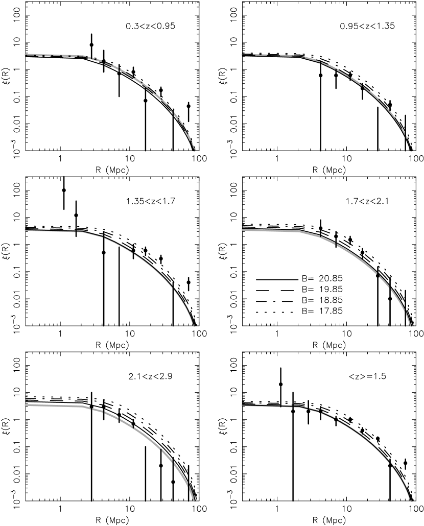
Figure 1: Predicted correlation function at various redshifts, in comparison to the 2dF data (Croom et al. 2001b). The dark lines show the correlation function predictions for quasars of various apparent B-band magnitudes ($B$). The 2dF limit is $B\sim 20.85$. The lower right panel shows data from entire 2dF sample in comparison to the theoretical prediction at the mean quasar redshift of $\langle z\rangle=1.5$. The $B=20.85$ prediction at this redshift is also shown by thick gray lines in the other panels to guide the eye. This case assumes $M_{\rm bh}\propto v_{c}^{5}$, normalized to local observations, and $\eta=1$ (case AI).

4 Comparison to Observations

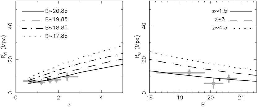
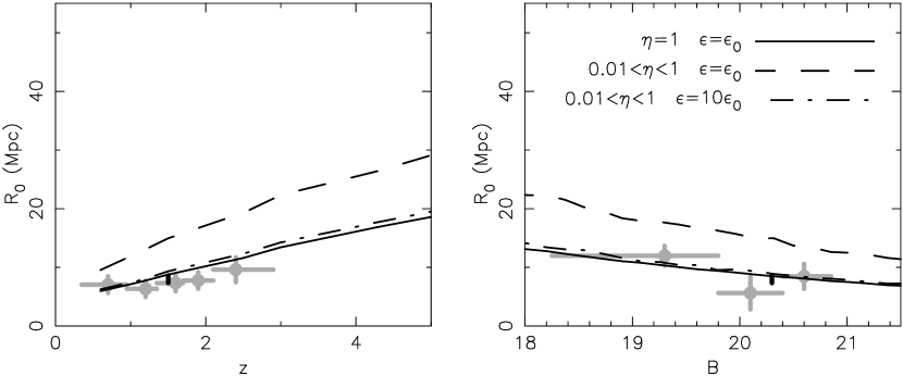
Figure 2: The correlation length, $R_{0}$ [defined through $\xi_{\rm q}(R_{0})=1$] plotted as a function of redshift (left hand panel) and apparent magnitude (right hand panel). The data is from the 2dF quasar redshift survey (Croom et al. 2001b,c), with the gray error bars showing the correlation length from different sub-samples, and the dark error bar at $z=1.5$ (left hand panels) and $B=20.3$ (right hand panels) showing the correlation length for the full sample. The theoretical model assumes $M_{\rm bh}\propto v_{c}^{5}$. In the upper panels $\eta=1$ (case AI), and the curves are shown for different apparent magnitudes (left), and different redshifts (right). In the lower panels we show curves corresponding to different choices for $\eta$ and $\epsilon$, (cases AII and AIII) assuming $B=20.3$ and $z=1.5$ respectively.

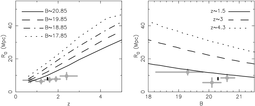
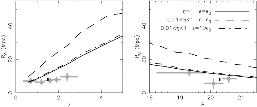
Figure 3: The correlation length, $R_{0}$ as a function of redshift (left hand panel) and apparent B-band magnitude (right hand panel). The data is from the 2dF QRS (Croom eta al. 2001b,c), with the gray error bars showing the correlation length from different sub-samples, and the dark error bars at $z=1.5$ (left hand panels) and $B=20.3$ (right hand panels) showing the correlation length for the full sample. The model assumes $M_{\rm bh}\propto M_{\rm halo}^{5/3}$. In the upper panels $\eta=1$ (case BI), and the curves are shown for different apparent magnitudes (left), and different redshifts (right). In the lower panels we show curves corresponding to different choices for $\eta$ and $\epsilon$ (cases BII and BIII), assuming $B=20.3$ and $z=1.5$ respectively.

Next we compare model correlation functions to observations from the 2dF quasar redshift survey (Croom et al. 2001b,c). Figure 1 shows the correlation function obtained by assuming that SMBH mass scales with halo circular velocity and that all quasars shine at their Eddington luminosity (case AI). We show the predicted correlation function at various redshifts, and several apparent B-band magnitudes, as determined from the relation

$$B = 5.5-2.5\log_{10}\left(\frac{L_{\rm B}}{L_{{\rm B},\odot}}\right)+5\log_{10}\left(\frac{D_{\rm L}}{10\mbox{pc}}\right)$$ (9)

$$- 2.5(1+\alpha_{\nu})\log_{10}\left(1+z\right),$$

where $\alpha_{\nu}=-0.5$ is the typical slope of the quasar power-law continuum (with a frequency dependence of the spectral flux $f_{\nu}\propto\nu^{\alpha_{\nu}}$), and $D_{\rm L}$ is the luminosity distance. The magnitude limit of the 2dF quasar redshift survey is $B\sim 20.85$, and so the data should be compared with the model correlation function corresponding to $B\sim 20-21$ (solid and dashed lines). The lower right panel of Figure 1 shows the 2dF correlation function generated from the entire quasar sample. This data is compared with a model correlation function computed at the median quasar redshift of the survey ($\langle z\rangle\sim 1.5$). The $B=20.85$ prediction at this redshift is replotted in the other panels of figure 1 to guide the eye (thick gray curves). We find that the correlation function depends more sensitively on redshift than on luminosity over the ranges under consideration.

4.1 The correlation function for models with $M_{\rm bh}\propto v_{\rm c}^{5}$

Variation of clustering with redshift and apparent magnitude is demonstrated more clearly in Figure 2. The upper panels show the dependences of the clustering length, $R_{0}$ [defined through the condition $\xi_{\rm q}(R_{0})=1$] for the fiducial case where the SMBH mass scales with halo circular velocity and quasars shine at their Eddington limit (case AI). The correlation length is plotted for various values of apparent magnitude as a function of redshift (left panel), and various redshifts as a function of apparent magnitude (right panel). The data for the correlation length as a function of redshift was computed from a sample having $B\lesssim 20.85$, drawn from the 2dF quasar redshift survey (Croom et al. 2001b,c). The gray error bars show the values for $R_{0}$ in different redshift bins, while the correlation length measured for the whole sample (plotted at $z=1.5$ and $B=20.3$ in the left and right hand panels respectively) is shown by the dark error bar. We find the predictions for $R_{0}$ to be consistent with observations. In particular, both the value of the clustering length and its slow evolution with redshift and apparent magnitude are consistent with current data. There is little variation of the clustering length with apparent magnitude over the range considered, although there is a tendency for brighter quasars to be more highly clustered, as was noted by Croom et al. (2002).

Note that the K-correction assumed in equation (9) is only valid out to $z\sim 3$ where Ly$\alpha$ absorption enters into the $B$-band. As a result the extrapolations of redshift dependence to $z\gtrsim 3$ shown in Figures 2 and 3 do not include Ly$\alpha$ absorption in the calculation of the quasar luminosity. However, these extrapolations are included to illustrate the evolution of the clustering length at yet higher redshifts (as measured in bands redward of the redshifted Ly$\alpha$ line).

The lower panels of Figure 2 show the corresponding dependence of the clustering length on redshift and apparent magnitude for quasars that shine at Eddington fractions $\eta$ lower than unity. Only the cases of $B=20.3$, corresponding approximately to the median quasar B-magnitude (left hand panel) and $z=1.5$ (right hand panel) are shown, and the curve corresponding to $\eta=1$ (case AI) is reproduced from the upper panels for comparison (solid lines). Assuming the local normalization $\epsilon=\epsilon_{\rm SIS}$ and that $\eta$ ranges between 0.01 and 1 with a constant $dP_{\rm obs}/d(\log\eta)$ (case AII), the typical quasar of apparent magnitude $B$ must be powered by a more massive SMBH and hence reside in a more massive galaxy than in the $\eta=1$ case. This results in a larger clustering length for quasars of a given apparent magnitude $B$. The resulting evolution, indicated by the dashed lines, appears to be incompatible with the data. The increase in $R_{0}$ may be compensated for by an increase in the normalization of the $M_{\rm BH}-M_{\rm halo}$ relation. The dot-dashed curves show the result of increasing this normalization relative to local observations by a factor of 10 ($\epsilon=10\epsilon_{\rm SIS}$). This factor equals the inverse of the median of the distribution $dP/d(\log{\eta})=\mbox{const}$. The resulting curve (corresponding to case AIII) is very similar to our fiducial case ($\eta=1$).

These results demonstrate that while a spread in the values of $\eta$ for different quasars results in the correlation function being measured over a wider range of halo masses, the correlation length is primarily sensitive to the characteristic halo mass, as specified by the characteristic value of $\eta$. Furthermore, the results demonstrate the important point that the correlation length measures the product of the normalization in the $M_{\rm bh}$–$M_{\rm halo}$ relation and the median fraction of the Eddington luminosity at which quasars shine, $\eta_{\rm med}$. With respect to the correlation function, this quantity $\epsilon\eta_{\rm med}$ (which is the same in cases AI and AIII) is more fundamental to the correlation function than the quasar lifetime since it predicts the correlation length independent from consideration of quasar number counts. It is important to note that since the normalization of the local $M_{\rm BH}-M_{\rm halo}$ relation is estimated ($\epsilon=\epsilon_{\rm SIS}$, Ferrarese 2002), the value of the quasar correlation length at low redshift implies that quasars spend most of their bright phase shining near their Eddington luminosity.

4.2 The correlation function for models with $M_{\rm bh}\propto M_{\rm halo}^{5/3}$

We next examine whether the correlation function observed by the 2dF survey may be used to constrain the evolution of the $M_{\rm bh}$–$M_{\rm halo}$ relation. In the previous sub-section, we have considered the case of a SMBH mass that scales with the fifth power of circular velocity independent of redshift (equation 7, case A). The alternative case B example postulates that the SMBH mass has a redshift independent scaling with the halo mass rather than halo circular velocity (equation 8). The upper panels of Figure 3 plot the correlation length in this case with $\eta=1$ and $\epsilon=\epsilon_{\rm SIS}$ (case BI). Both the evolution of the correlation length with redshift for different apparent magnitudes (left hand panel), and the variation of correlation length with a given apparent magnitude at various redshifts (right hand panel) are shown. The case B $M_{\rm bh}-M_{\rm halo}$ relation results in a correlation length that varies significantly more with redshift than the data requires. The lower panels show examples with values of $\eta$ that differ from unity. Only the cases of $B=20.3$ (left hand panel) and $z=1.5$ (right hand panel) are shown, and the result assuming $\eta=1$ (case BI) is reproduced from the upper panels for comparison (solid lines). If $\epsilon=\epsilon_{\rm SIS}$, and $\eta$ ranges between 0.01 and 1, with $dP_{\rm obs}/d\eta\propto\mbox{const}$ (case BII), then the typical quasar of apparent magnitude $B$ must have a larger clustering length (dashed lines). This may be compensated for by increasing the normalization of the $M_{\rm BH}$–$M_{\rm halo}$ relation by a factor of 10 ($\epsilon=10\epsilon_{\rm SIS}$, case BIII) as considered before (dot-dashed lines).

The rapid evolution with redshift that results from a case B $M_{\rm BH}$–$M_{\rm halo}$ relation could be diminished if the luminosities of quasars were a higher fraction of their Eddington limit at higher redshift. However we have seen that the locally observed normalization of the $M_{\rm bh}$–$M_{\rm halo}$ relation requires most present-day quasars to be shining near their Eddington luminosity. Quasars at high redshift would therefore have to be super-Eddington, shining at $\sim\eta\sim(1+z)^{5/2}$ ($\eta\sim 30$ at $z\sim 3$) in order to reproduce the observed slow evolution of the clustering length. This requirement on $\eta$ may be somewhat relaxed in models having $\epsilon>\epsilon_{\rm SIS}$, as is discussed in the next section.

5 Constraining $\eta$ and $\epsilon$ using the quasar correlation function

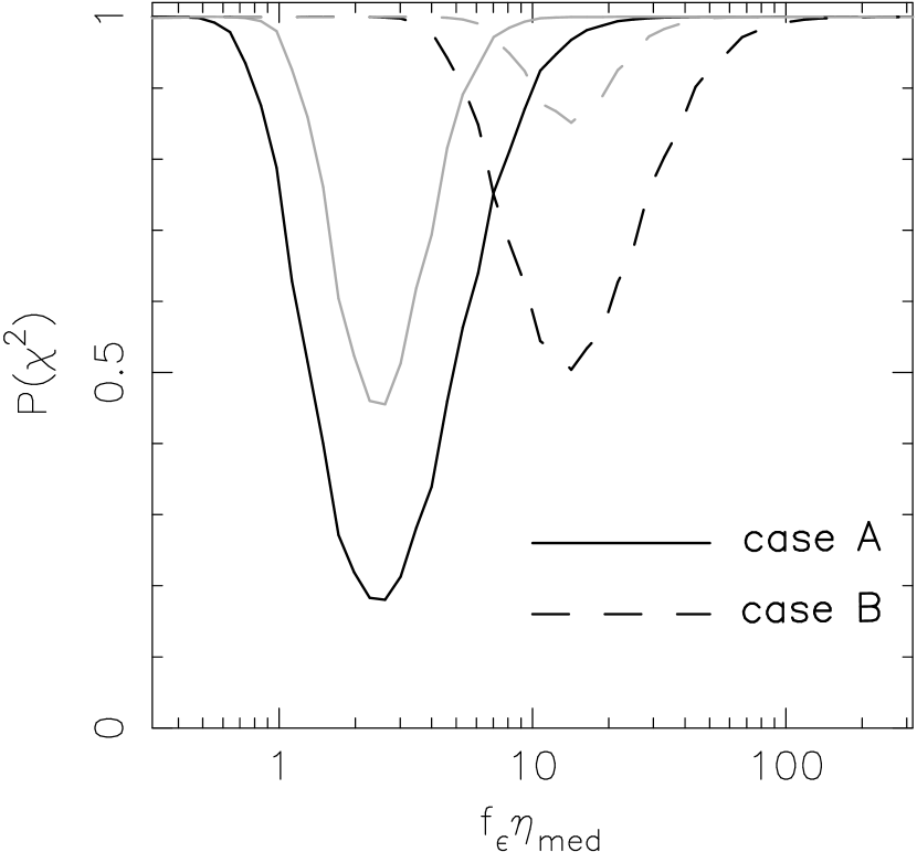
Figure 4: The probability $P(\chi^{2})$ of case A and case B models as a function of $f_{\epsilon}\eta_{\rm med}$. The dark lines correspond to fits to the redshift dependent correlation length $R_{0}(z)$ measured by the 2dF quasar redshift survey (Croom et al. 2001b). The gray lines show results for a hypothetical larger future sample whose errors on $R_{0}$ are reduced by a factor of $\sqrt{2}$ relative the the 2dF quasar survey.

The $M_{\rm bh}$–$M_{\rm halo}$ relation for local galaxies requires a choice for the relationship between the circular velocity at the radius probed by observations of galaxies, and the circular velocity at the virial radius. This relationship depends on the dark-matter mass profile and is still uncertain due to the gravitational interaction between the baryons (which cool and often dominate gravity near the center of galaxies) and the dark matter. Ferrarese (2002) presented $M_{\rm bh}$–$M_{\rm halo}$ relations for three different cases, which may be summarized in the present notation by $\epsilon=\epsilon_{\rm SIS}$, $\epsilon=\epsilon_{\rm NFW}=3.7\epsilon_{\rm SIS}$, and $\epsilon=\epsilon_{\rm S02}=25\epsilon_{\rm SIS}$. The second case corresponds to the universal profile of Navarro, Frenk & White (1996, NFW), and the third to the normalization derived based on the weak lensing study of Seljak (2002).

The results in the preceding sections have been presented for fiducial models with $(\epsilon,\eta)=(\epsilon_{\rm SIS},1)$, ($\epsilon_{\rm SIS},0.1$) and ($10\epsilon_{\rm SIS},0.1$). It was demonstrated that the correlation function is primarily dependent on the product between $\epsilon$ and the median value of $\eta$, namely $\epsilon\eta_{\rm med}$. This raises the possibility that $\epsilon\eta_{\rm med}$ could be constrained using correlation function data. We have computed the evolution of the correlation length $R_{0}(z)$ for a set of models having a range of values for the product $\epsilon\eta_{\rm med}\equiv f_{\epsilon}\epsilon_{\rm SIS}\eta_{\rm med}$, and calculated the reduced $\chi^{2}$-statistics as well as the confidence with which a model is excluded by the 2dF data, $P(\chi^{2})$. In figure 4 we plot the resulting $P(\chi^{2})$ as a function of $f_{\epsilon}\eta_{\rm med}$ (dark lines).

The results suggest that Case A models (solid lines) favor $f_{\epsilon}\eta_{\rm med}\sim 1$–$5$ indicating that $\epsilon$ is a factor of a few larger than $\epsilon_{\rm SIS}$ for $\eta\sim 1$, as would be expected from the universal NFW profile, or that $\eta_{\rm med}$ has a maximum value of a few tenths. If $\epsilon=\epsilon_{\rm S02}$, case A requires $\eta_{\rm med}\sim 0.08$. Figure 4 shows that Case B models (dashed lines) are more restricted, requiring $f_{\epsilon}\eta_{\rm med}\sim 10-30$. This implies that $\epsilon=\epsilon_{\rm SIS}$ and $\epsilon=\epsilon_{\rm NFW}$ cannot be accommodated since the required values of $\eta_{\rm med}\gtrsim 10$ and $\eta_{\rm med}\gtrsim 3$ respectively, are considered unphysical in most accretion models (Nityananda & Narayan 1982; see, however, Ruszkowski & Begelman 2003). The more extreme case of $\epsilon=\epsilon_{\rm S02}$ may be marginally accommodated by case B; however even in this case the quasars must shine somewhat in excess of their Eddington limit.

Figure 4 also shows $P(\chi^{2})$ as a function of $f_{\epsilon}\eta_{\rm med}$ for a hypothetical future survey that would yield the same evolution of $R_{0}$ with redshift, but with errors that are smaller by a factor of $\sqrt{2}$ (light lines). Future surveys will better constrain the gradient $dR_{0}/dz$, and help discriminate further between different models of the $M_{\rm bh}$–$M_{\rm halo}$ relation.

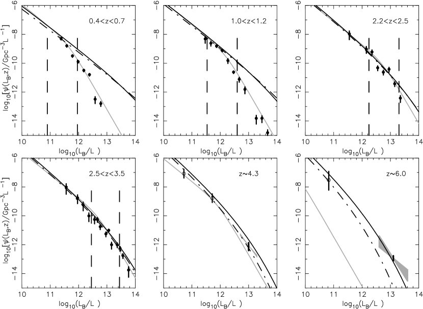
Figure 5: Comparison of the model and observed quasar luminosity functions at various redshifts. The data points at $z\lesssim 4$ are summarized in Pei (1995), while the light lines show the double power-law fit to the 2dF quasar luminosity function (Boyle et al. 2000). At $z\sim 4.3$ and $z\sim 6.0$ the data is from Fan et al. (2001a;2001b;2003). The gray regions show the 1-$\sigma$ range of logarithmic slope ($[-2.25,-2.75]$ at $z\sim 4.3$ and $[-1.6,-3.1]$ at $z\sim 6$), and the vertical bars show the uncertainty in the normalization. The open circles show data points converted from the X-ray luminosity function (Barger et al. 2003) of low luminosity quasars using the median quasar spectral energy distribution (Elvis et al. 1994). The model luminosity functions shown correspond to cases AI (solid curves) and a model assuming case B evolution with $\epsilon=\epsilon_{\rm S02}$, $\eta=1$ and a constant lifetime of $t_{\rm q}=10^{7}$ years (dot-dashed curves). The dashed pairs of vertical lines show the range corresponding to apparent B-magnitudes between 18.25 and 20.85.

Our discussion so far has been independent of the quasar luminosity function. In the next section we discuss how the luminosity function may be used to determine the redshift evolution of the quasar lifetime.

6 The Luminosity Function and Quasar Lifetime

In the previous sections we have demonstrated that the evolution of the $M_{\rm bh}$–$M_{\rm halo}$ relation with redshift may be constrained directly from the quasar correlation function. We have shown that the critical parameter determining the SMBH mass is the halo circular velocity rather than the halo mass. We reiterate that this result does not rely on the luminosity function of quasars. On the other hand, the number counts of quasars are proportional to the quasar lifetime. Therefore, the quasar lifetime and its evolution with redshift may be determined by comparing the observed quasar number counts to the SMBH mass function. The latter may be obtained from the Press-Schechter (1976) mass-function of dark-matter halos (with the improvement of Sheth & Tormen 1999) combined with the $M_{\rm bh}$–$M_{\rm halo}$ relation.

Theoretical models of the quasar luminosity function often associate quasar activity with major mergers (e.g. Kauffmann & Haehnelt 2000; Wyithe & Loeb 2003). A simple model that attributes quasar activity to major mergers, assumes a $M_{\rm bh}$–$M_{\rm halo}$ relation that is described by equation (7), and sets the quasar lifetime equal to the dynamical time of a galactic disk, accurately reproduces the entire optical and X-ray luminosity functions of quasars at redshifts between 2 and 6 (Wyithe & Loeb 2003). At lower redshifts ($z\lesssim 2$), this prescription correctly predicts the luminosity function at luminosities below the characteristic break (Boyle et al. 2000). In difference to Wyithe & Loeb (2003) we have assumed the quasar activity to take place in the larger SMBH before coalescence of the SMBH binary formed during the merger (Volonteri et al. 2002). Figure 5 shows the comparison of this model with observations. Specifically, we show the fiducial case AI (which corresponds to the model presented in Wyithe & Loeb 2003) using equation (7) with $\epsilon=\epsilon_{\rm SIS}$ and $\eta=1$ (solid curves). We have shown that case AI describes the observed quasar correlation function (see figures 1-2). However as discussed in § 5, case-B models for the $M_{\rm bh}$–$M_{\rm halo}$ relation also provide acceptable fits to $R_{0}(z)$ so long as $\epsilon\gtrsim 10\epsilon_{\rm SIS}$ and $\eta\sim 1$. Therefore a corresponding luminosity function model was also generated for this case assuming a constant lifetime of $t_{\rm q}=10^{7}$ years. We have plotted this model in figure 5 (dot-dashed lines).

We find that our fiducial model (case AI; solid lines) with a quasar lifetime that equals the dynamical time of a galactic disk, reproduces the observed luminosity function over a wide range of redshifts and luminosities (see Wyithe & Loeb 2003). Our second model (case B, $\epsilon\gtrsim 10\epsilon_{\rm SIS}$, $\eta=1$, $t_{\rm q}=10^{7}$; dot-dashed lines) also reproduces the observed luminosity function at $z\lesssim 4.5$. However at $z\sim 6$ this model underestimates the observed number counts by two orders of magnitude. Case B evolution for the $M_{\rm bh}$–$M_{\rm halo}$ relation is therefore challenged by the existence of the highest redshift quasars, which would imply a quasar lifetime that exceeds the age of the universe at $z\sim 6$. Moreover, given the Salpeter (1964) time of $\sim 4\times 10^{7}$ years, the SMBHs powering these quasars would grow to 25 times their initial mass during their lifetime. Provided that quasar activity is trigged by major mergers, the requirement that the $M_{\rm bh}$–$M_{\rm halo}$ relation reproduce the observed evolution in quasar clustering, together with the observed evolution in the number counts of quasars therefore implies case A evolution, and a quasar lifetime that is set by the dynamical time of the host galaxy. We reinforce the important qualitative result that since the evolution of quasar correlations require SMBHs to take a larger fraction of the halo mass at high redshift (case A, see equation 7), the observed evolution in the number counts requires a quasar lifetime that is shorter at higher redshifts, scaling approximately as the dynamical time of a dark matter halo [$\propto(1+z)^{-3/2}$].

We point out that the model luminosity functions fail to reproduce the rapid drop in the density of luminous quasars seen at low redshift. This drop is thought to be due to the consumption of cold gas in galaxies by star formation (e.g. Kauffmann & Haehnelt 2000) and the inhibition of accretion onto massive halos at late times (e.g. Scannapieco & Oh 2004). However, most of the quasars in the 2dF quasar redshift survey have $B$-magnitudes that lie below the characteristic break in the luminosity function at low redshift (Boyle et al. 2000; Croom et al. 2001). This can be seen in Figure 5 where the vertical dashed lines show the luminosities bracketing the apparent magnitude range $18.25<B<20.85$. Since the model correctly predicts the luminosity function within most of this luminosity range at all redshifts, we are justified in deriving combined constraints from the luminosity and correlation functions of quasars.

7 Do bright low-redshift quasars shine near their Eddington Luminosity?

In § 4 we demonstrated that the 2dF quasar sample has a correlation length that is consistent with the local $M_{\rm bh}-M_{\rm halo}$ relation, and that quasars shine near their Eddington luminosity. In addition it was shown that this consistency extends to both bright and faint subsamples of quasars. The brightest 2dF quasars ($18.1\leq B\leq 19.9$) presented by Croom et al. (2002) are mostly brighter than the characteristic break luminosity in the differential quasar number counts (e.g. Boyle et al. 2000). These bright quasars have a lower abundance than expected from merging halos at $z\lesssim 2$ (see figure 5). Either the lifetime (or occupation fraction) of bright quasars is lower than expected at $z\lesssim 2$ or else these quasars shine well below their Eddington limit. Figure 2 indicates that the slow dependence of $R_{0}$ with $B$ reported by Croom et al. (2002) is consistent with the expected trend if all quasars shine near their Eddington luminosity. This consistency suggests that bright quasars are under represented at $z\lesssim 2$ because of a reduced quasar lifetime (or a reduced occupation fraction) rather than a reduced value of $\eta$ during their brightest phase.

8 discussion

In this paper we have demonstrated that the relationship between the mass of a SMBH and its host dark-matter halo is the fundamental quantity that determines the clustering of quasars. In particular the $M_{\rm bh}$–$M_{\rm halo}$ relation and its evolution with redshift, may be determined directly from the evolution in the correlation length of quasars, independent of consideration of the quasar luminosity function or assumptions about the quasar lifetime. Beginning with the locally observed $M_{\rm bh}$–$M_{\rm halo}$ relation, we have shown that the observed correlation length of quasars in the 2dF quasar redshift survey is consistent with SMBHs that shine at $\sim 10$–$100\%$ of their Eddington luminosity during their bright quasar episode. Moreover, the evolution of the clustering length with redshift is consistent with a SMBH mass whose redshift-independent scaling is with the circular velocity of the host dark matter halo (see equation 7). In contrast, it appears that a relation for the SMBH mass whose redshift-independent scaling is with the mass of the host dark matter halo (equation 8) would have resulted in too much evolution of the clustering length with redshift.

The portion of the 2dF quasar survey from which the data used in this study were drawn, contains $\sim 10^{4}$ quasars. Upon completion, the Sloan Digital Sky Survey will have spectra for ten times this number of quasars, spread over a larger redshift range (York et al. 2000). This will allow more accurate determination of the correlation length and its evolution, and hence provide more accurate constraints the SMBH population. The selection of quasars for the spectroscopic survey of SDSS at $z<3$ is restricted to $i^{*}<19$. Thus, most of the low redshift SDSS quasars will fall at luminosities that are brighter than the characteristic break in the luminosity function (e.g. Boyle et al. 2000). These bright quasars have a lower abundance than expected from the number of halos merging at $z\lesssim 2$. The reason for this low abundance may be either that the lifetime (or occupation fraction) of bright quasars is lower than expected at $z\lesssim 2$, or alternatively that the fraction of the Eddington limit at which the quasars shine is small. The 2dF quasar sample straddles the luminosity function break. We have shown that the similarity in the clustering statistics of sub-samples of quasars having different ranges in luminosity suggest that the lifetime (or occupation fraction) of bright quasars is lower than expected at $z\lesssim 2$, but that these quasars also shine near their Eddington luminosity. Measurements of the correlation length as a function of quasar luminosity in SDSS can help further distinguish between these two possibilities.

As we have shown in a previous paper (Wyithe & Loeb 2003), feedback–regulated growth of SMBHs during active quasar phases implies $M_{\rm bh}\propto v_{c}^{5}$, consistent with the inferred relation for galactic halos in the local universe (Ferrarese 2002). Assuming $\eta=1$ as suggested by observations of both low and high-redshift quasars (Floyd 2003; Willott, McLure & Jarvis 2003), we have shown that only $\sim 7\%$ of the Eddington luminosity output needs to be deposited into the surrounding gas in order to unbind it from the host galaxy over the dynamical time of the surrounding galactic disk. The power-law index of 5 in the $M_{\rm bh}$–$v_{c}$ relation, is larger than the values of 4–4.5 inferred from the local relation between $M_{\rm bh}$ and the stellar velocity dispersion $\sigma_{\star}$ (Merritt & Ferrarese 2001; Tremaine et al. 2002); the difference originating from the observation that the $v_{c}$–$\sigma_{\star}$ relation is shallower than linear for stellar bulges embedded in cold dark matter halos (Ferrarese 2002). Feedback–regulated growth also implies that the $M_{\rm bh}$–$v_{\rm c}$ relation should be independent of redshift, as implied by the slow evolution in the clustering length of quasars.

A very simple model can therefore be constructed to describe the correlation length of quasars and its evolution in the 2dF survey, as well as the number counts of quasars out to very high redshift ($z\sim 6$). The model includes four simple assumptions, but no free parameters: (i) the locally observed $M_{\rm bh}$–$M_{\rm halo}$ relation extends to high redshifts through equation (7) with the SMBH mass scaling as halo circular velocity to the 5-th power; (ii) SMBHs shine near their Eddington luminosity with a universal spectrum (Elvis et al. 1994) during luminous quasar episodes; (iii) quasar episodes are associated with major galaxy mergers; and (iv) the quasar lifetime is set by the dynamical time of the host galaxy.

The assumption of a SMBH mass that scales with halo circular velocity independently of redshift is supported by the observations of Shields et al. (2003) that there is no evolution in the $M_{\rm bh}$–$\sigma_{\star}$ relation out to $z\sim 3$. The assumption that quasars shine near their Eddington limit is supported by observations of high and low redshift quasars (Floyd 2003; Willott, McLure & Jarvis 2003). Overall, the sample of available data on the clustering properties and the number counts of quasars is most readily explained by a quasar lifetime that is set by the dynamical time of the host galaxy rather than by the Salpeter (1964) $e$-folding time for the growth of its mass.

References

- Barger et al. (2003) Barger, A. J., Cowie, L. L., Capak, P., Alexander, D. M., Bauer, F. E., Brandt, W. N., Garmire, G. P., & Hornschemeier, A. E. 2003, astro-ph/0301232
- (2) Barkana, R., & Loeb, A. 2001, Phys. Rep., 349, 125
- Boyle et al. (2000) Boyle, B. J., Shanks, T., Croom, S. M., Smith, R. J., Miller, L., Loaring, N., & Heymans, C. 2000, MNRAS, 317, 1014
- Croom et al. (2001) Croom, S. M., Smith, R. J., Boyle, B. J., Shanks, T., Loaring, N. S., Miller, L., & Lewis, I. J. 2001a, MNRAS, 322, L29
- Croom et al. (2001) Croom, S. M., Shanks, T., Boyle, B. J., Smith, R. J., Miller, L., Loaring, N. S., & Hoyle, F. 2001b, MNRAS, 325, 483
- Croom et al. (2002) Croom, S. M., Boyle, B. J., Loaring, N. S., Miller, L., Outram, P. J., Shanks, T., & Smith, R. J. 2002, MNRAS, 335, 459
- Elvis et al. (1994) Elvis, M. et al. 1994, ApJS, 95, 1
- (8) Fan, X., et al. 2001a AJ, 121, 54
- (9) Fan, X., et al. 2001b AJ, 122, 2833
- (10) Fan, X., et al. 2003, astro-ph/0301135
- Ferrarese (2002) Ferrarese, L. 2002, ApJ, 578, 90
- (12) Floyd, D.J.E., 2003, astro-ph/0303037
- Goldschmidt & Miller (1998) Goldschmidt, P. & Miller, L. 1998, MNRAS, 293, 107
- Haiman & Hui (2001) Haiman, Z. & Hui, L. 2001, ApJ, 547, 27
- (15) Jakobsen, P., Jansen, R., A., Wagner, S., Reimers, D., 2003, Astron. Astrophys, 397, 891
- Kauffmann & Haehnelt (2000) Kauffmann, G. & Haehnelt, M. 2000, MNRAS, 311, 576
- Kauffmann & Haehnelt (2002) Kauffmann, G. & Haehnelt, M. G. 2002, MNRAS, 332, 529
- (18) Magorrian, J. et al. 1998, AJ, 115, 2285
- Martini (2003) Martini (2003) Martini, P. 2003, preprint astro-ph/0304009
- Martini & Weinberg (2001) Martini, P. & Weinberg, D. H. 2001, ApJ, 547, 12
- McLure & Dunlop (2002) McLure, R. J. & Dunlop, J. S. 2002, MNRAS, 331, 795
- (22) Merritt, D., & Ferrarese, L., 2001, ApJ., 547, 140
- Mo & White (1996) Mo, H. J. & White, S. D. M. 1996, MNRAS, 282, 347
- Nityananda & Narayan (1982) Nityananda, R. & Narayan, R. 1982, MNRAS, 201, 697
- (25) Pei, Y. C. 1995, ApJ, 438, 623
- (26) Press, W. H., & Schechter, P. 1974, ApJ, 187, 425
- Ruszkowski & Begelman (2003) Ruszkowski, M. & Begelman, M. C. 2003, ApJ, 586, 384
- Salpeter (1964) Salpeter, E. E. 1964, ApJ, 140, 796
- Sheth & Tormen (1999) Sheth, R. K. & Tormen, G. 1999, MNRAS, 308, 119
- (30) Scannapieco, E., Oh, S.P., 2004, astro-ph/0401087
- Seljak (2002) Seljak, U. 2002, MNRAS, 334, 797
- Sheth, Mo, & Tormen (2001) Sheth, R. K., Mo, H. J., & Tormen, G. 2001, MNRAS, 323, 1
- Shields et al. (2003) Shields, G. A., Gebhardt, K., Salviander, S., Wills, B. J., Xie, B., Brotherton, M. S., Yuan, J., & Dietrich, M. 2003, ApJ, 583, 124
- Silk & Rees (1998) Silk, J. & Rees, M. J. 1998, A&A, 331, L1
- Spergel et al. (2003) Spergel, D. N. et al. 2003, ApJS, 148, 175
- Tremaine et al. (2002) Tremaine, S. et al. 2002, ApJ, 574, 740
- Volonteri, Haardt, & Madau (2003) Volonteri, M., Haardt, F., & Madau, P. 2003, ApJ, 582, 559
- Willott, McLure, & Jarvis (2003) Willott, C. J., McLure, R. J., & Jarvis, M. J. 2003, astro-ph/0303062
- Wyithe & Loeb (2003) Wyithe, J. S. B. & Loeb, A. 2003, ApJ, 595, 614
- York et al. (2000) York, D. G. et al. 2000, AJ, 120, 1579
- (41) Yu, Q., & Tremaine, S. 2002, MNRAS, 335, 965