HST ABSOLUTE SPECTROPHOTOMETRY OF VEGA FROM THE FAR-UV TO THE IR

Abstract

The Space Telescope Imaging Spectrograph has measured the absolute flux for Vega from 0.17–1.01 $\mu$m on the HST White Dwarf flux scale. These data are saturated by up to a factor of 80 overexposure but retain linearity to a precision of 0.2%, because the charge bleeds along the columns and is recovered during readout of the CCD. The S/N per pixel exceeds 1000, and the resolution $R$ is about 500. A $V$ magnitude of 0.026$\pm$0.008 is established for Vega; and the absolute flux level is $3.46\times 10^{-9}$ erg cm^-2 s^-1 at 5556 Å. In the regions of Balmer and Paschen lines, the STIS equivalent widths differ from the pioneering work of Hayes in 1985 but do agree with predictions of a Kurucz model atmosphere, so that the STIS flux distribution is preferred to that of Hayes. Over the full wavelength range, the model atmosphere calculation shows excellent agreement with the STIS flux distribution and is used to extrapolate predicted fluxes into the IR region. However, the IR fluxes are 2% low with respect to the standard Vega model of Cohen. IUE data provide the extension of the measured STIS flux distribution from 0.17 down to 0.12 $\mu$m. The STIS relative flux calibration is based on model atmosphere calculations of pure hydrogen WDs, while the Hayes flux calibration is based on the physics of laboratory lamps and black body ovens. The agreement to 1% of these two independent methods for determining the relative stellar flux distributions suggests that both methods may be correct from 0.5–0.8 $\mu$m and adds confidence to claims that the fluxes relative to 5500 Å are determined to better than 4% by the pure hydrogen WD models from 0.12 to 3 $\mu$m.

To be published in the 4 June 2004 issue of the Astronomical Journal

1. INTRODUCTION

The most commonly used flux calibration for the fundamental standard Vega ($\alpha$ Lyr, HD 172167, HR 7001) is the compilation of Hayes (1985), while Megessier (1995) suggests an increase of 0.6% in the Hayes value of $3.44\times 10^{-9}$ erg cm^-2 s^-1 Å^-1 at 5556 Å. The Hayes flux for Vega is traceable to fundamental standard lamps pedigreed by NBS (now NIST), which is charged with maintaining fundamental standards of physical units. The Hayes flux compilation is based on direct comparisons of the star to calibrated lamps and black body ovens. Most ground based estimates of absolute stellar flux are traceable to the flux of Vega.

With the advent of extensive space based observations in the far-UV, a need for standard flux candles arose at wavelengths below the atmospheric cutoff. A few rocket experiments established some UV standard stars with $\sim$10% precision (e.g.  Strongylis & Bohlin 1979). To establish standards with better accuracy, a technique based on model atmospheres for simple, pure hydrogen WDs was suggested by D. Finley and J. Holberg for calibrating the IUE satellite spectrophotometry, (cf. Fig. 8 in Bohlin, et al. 1990). The hot WD standard stars G191B2B, GD 153, and GD 71 at $V=12$–13 mag were established by computing LTE model atmosphere flux distributions for pure hydrogen atmospheres, which were then normalized to precisely measured $V$ magnitudes from A. Landolt (see Bohlin 2000). EUV observations below the Lyman limit demonstrated that any effects of interstellar extinction in these three stars is less than 1% longward of the 912 Å Lyman limit. These three WD standards are now based on NLTE models by Ivan Hubeny (Bohlin 2003) and are complemented by three solar analog stars for HST calibrations extending into the IR (Bohlin, Dickinson, & Calzetti 2001).

The Vega observations with STIS are discussed in Section 2. Section 3 establishes the best estimate of the V band magnitude of Vega, while Section 4 presents the first direct comparison between the WD and the standard lamp methods for establishing absolute flux. A third method for defining the flux of Vega at all wavelengths is based on modeling of its stellar atmosphere, as discussed in Section 5. Model atmosphere codes are now sophisticated enough to warrant detailed comparisons between observation and theory. Because of the excellent agreement of a model (Kurucz 2003, Castelli and Kurucz 1994) with the STIS observations up to 1 $\mu$m, the model should provide a good estimate of the flux beyond 1 $\mu$m, as discussed in Section 6.

2. CALIBRATION OF THE SATURATED OBSERVATIONS

STIS observations of Vega in the three CCD low dispersion modes G230LB, G430L, and G750L (Kim Quijano 2003) produce heavy saturation of the full well depth. However at Gain = 4, the A-to-D amplifier does not saturate; and the excess charge just bleeds into adjacent pixels along the columns, which are perpendicular to the dispersion axis. Gilliland, Goudfrooij, and Kimble (1999, GGK) have demonstrated that saturated data on the STIS CCD are linear in total charge vs. stellar flux, as long as the extraction region on the CCD image is large enough to include all the charge. In particular, GGK demonstrated linearity to 0.1% accuracy using 50$\times$ overexposed images of a star in M67 to compare with unsaturated exposures of the same star. In the G430M medium dispersion spectral mode, 0.8s observations of $\alpha$ Cen A saturated by about a factor of 4; and GGK showed that the ratio to a mean G430M spectrum at 0.1s is linear to $\ll 1$%. Furthermore, GGK demonstrated that the short 0.3s STIS exposure times are stable and accurate to 0.2%, i.e. 0.0006s.

2.1. Corrections for the Tall Extractions of the Saturated Data

For Vega, the extraction heights required to include all the charge in the saturated images are 84, 54, and 40 pixels tall for G230LB, G430L, and G750L, respectively, for single integrations of 6s for G230LB and 0.3s for G430L and G750L. For these saturated images, the signal level is so high that any signal loss due to charge transfer efficiency (CTE) effects (Bohlin & Goudfrooij 2003) is $<$0.1%.

Because of scattered light from the STIS gratings, a tall extraction height contains more signal than the standard 7 pixel extraction, to which the absolute flux calibrations apply (Bohlin 1998). The amount of excess signal in the tall extractions must be derived from unsaturated images. Observations of the star AGK+81^∘266 that is used to monitor the change in STIS instrumental sensitivity are used to derive the correction for the heights of 54 and 40 pixels, respectively for G430L with 43 observations and G750L with 37 observations. For G230LB, the three unsaturated G230LB observations of Vega itself are used to correct the 84 pixel extractions of the saturated observations. All three unsaturated Vega G230LB spectra at the detector center give the same correction from a 7 to an 84 pixel high extraction. This correction drops from 1.293 at 1700 Å to 1.150 at 3000 Å with a maximum difference among the three observations of 0.2% in the 1.293 correction factor at 1700 Å.

The uncertainties in the tall slit corrections for G430L and for G750L below 8450 Å, where saturation ends (see 2.3 below), can be characterized by the rms scatter among the many AGK+81^∘266 determinations. The ratios of the 54 and 40 pixel high extractions to the standard 7 pixel extraction have an added uncertainty of 0.2–0.6% measured by the rms of these ratios for AGK+81^∘266 but do not show trends with time that might be caused by the increasing CTE losses. The CTE correction for the 7 pixel extractions grows from zero in 1997 to a maximum of 3% in the relevant 3000–8450 Å range for the AGK+81^∘266 data obtained near the time of the Vega observations; but the limit to any error caused by our assumption of a matching CTE correction in the 54 or 40 pixel tall extractions is included in the 0.2–0.6% rms values. For example in the range covered by the $V$ filter (see Section 3), the rms uncertainty in the tall slit correction is 0.3%. The rms uncertainties of $<$0.2% for G230LB and 0.2–0.6% over the 3000–8450 Å range for the tall slit correction ratios should be included in the total systematic error budget as a function of wavelength.

2.2. Verification of Linearity for Saturated Data

2.2.1 Shutter Timing

Linearity for the Vega data can be verified directly, because 0.3s observations of Vega in the G230LB mode are unsaturated below 2900 Å, i.e. over the first 900 pixels of the 1024 pixel spectrum. Exposures of 6s were obtained in order to re-verify linearity up to a saturation factor of 20. The 6s observations with G230LB are more saturated at the longest wavelengths than at any wavelength in the G430L or G750L spectra. Table 1 is the journal of the Vega observations, while Figure 1 demonstrates both the repeatability of G230LB observations and, also, the linearity beyond saturation. The individual frame exposure times are the exptime per cr-split frame from Table 1, i.e. 0.3s for all observations, except for the saturated G230LB observations of 6s. One spectrum in the 52X2E1 aperture was placed 130 pixels from the top of the detector, where the CTE correction is 4$\times$ lower than the central correction, which exceeds 1% only below 2000 Å. However, the flat field correction for the E1 position relative to centered spectra is currently based on only 13 observations obtained in 2000–2002 and is uncertain by $\sim$0.5%. The E1 exposure will not be included in the analysis below. Figure 1 shows the ratio of the five centered individual G230LB observations to their average. The two 6s exposures are low by 0.9998$\pm$0.0005 and the three centered and unsaturated ratios average 1.0027$\pm$0.0005. The discrepancy between the flux for the two exposure times is 0.29%$\pm$0.07%. One simple explanation is that the nominal 0.3s exposures are really 0.3009s$\pm$0.0002s, in agreement with GGK who find that the 0.3s shutter timing is accurate to $\sim$0.0006s.

2.2.2 Saturation and Charge Transfer Efficiency Corrections

Other possibilities for the 0.3% flux difference between the 0.3 and 6s exposures are non-linearities, either in the saturated data or in the CTE correction of the unsaturated data. GGK demonstrate linearity to better than 0.1% for exposures of point sources overexposed by 50$\times$ and for spectra of $\alpha$ Cen A at 4$\times$ over saturation (see above). The loss of signal due to charge transfer efficiency (CTE) is $<$0.1% for the saturated spectra, while the amount of the CTE correction for the unsaturated 0.3s G230LB data ranges from $\sim$1.5% at the shorter wavelengths to $\sim$0.5% at the longest wavelengths. Bohlin and Goudfrooij (2003) suggest their CTE correction formula is accurate to 10% for the signal level of the Vega data, which corresponds to $<$0.2% for the CTE correction of $<$2% for the 0.3s fluxes. Because these uncertainties are comparable to the measured timing error of the 0.3s exposures, the nominal 0.3000s value is retained. The uncertainty of 0.3% in the 0.3s exposure times will contribute to the uncertainty in the final determination of the measured STIS $V$ mag that will be compared with $V=0.035$, which was previously used to set the overall level of the absolute STIS flux calibration on the WD scale (Bohlin 2000 and Section 3 below.)

2.3. Additional Details

The 84 pixel extractions have more contamination from the out-of-band scattered light that fills in the line cores slightly and produces the $\sim$1% dips in Figure 1 at the locations of the deeper lines in the 7 pixel extractions from the 0.3s images. At the strong 2800 Å Mg II line, the differential filling reaches $\sim$2%. To minimize the out-of-band stray light, a standard 7 pixel extraction is used longward of 8450 Å, where there is no saturation in the 0.3s exposures with G750L.

After extracting the spectra from the images, adjusting the flux to a standard 7-pixel-high aperture, correcting for sensitivity changes with time Bohlin (2003), and applying the CTE correction (Bohlin & Goudfrooij 2003), corrections to the wavelengths are made for sub-pixel wavelength errors that are obvious in the high S/N saturated spectra. These shifts range up to 0.5 pixel and are found by cross-correlation of the absorption lines with a model flux distribution.

3. THE V BAND MAGNITUDE OF VEGA

The STIS flux calibration is based on standard star reference fluxes that are pure hydrogen WD models normalized relative to the average flux of Vega over the $V$ band (Colina and Bohlin 1994, Bohlin 2000). The absolute flux of these fundamental standard stars G191B2B, GD 71, and GD 153, depends directly on the difference between the $V$ magnitude of Vega and $V$ for each WD star. The one sigma uncertainties in the Landolt $V$ magnitudes of the WD stars are in the range 0.001–.004 mag (Landolt 1992 and private communication). The measured STIS flux for Vega relative to the WD standard star fluxes determines the instrumental $V$ magnitude of Vega with respect to the precision Landolt $V$ magnitudes of the WDs. The Landolt transformations from his instrumental scale to Johnson $V$ magnitudes is summarized in Colina and Bohlin (1994). There are three choices for the definition of the Landolt $V$ bandpass: the Kitt Peak filter+detector (Landolt, private communication), the CTIO filter+detector (Landolt 1992), and the latter as modified by Cohen et al.  (2003b) to include an estimate of the atmospheric transparency above the CTIO observatory. None of the estimated bandpass functions include the telescope optics; but that omission is expected to cause $<$0.001 mag errors (Colina and Bohlin 1994). The three bandpass functions yield slightly different magnitudes for Vega in the range of $V=0.021$ to 0.031; but $V=0.026$ for the Cohen et al. (2003b) bandpass with the atmosphere included should be the most accurate. Conservatively, 0.005 mag is assigned to the uncertainty that still remains in the Landolt-Cohen CTIO bandpass function. The small scatter of 0.002 among the separate determinations from the three WDs is included in the 0.005 mag bandpass error estimate.

Colina and Bohlin (1994) previously adopted $V=0.035$ for Vega. Megessier (1995) and Bessell, Castelli, and Plez (1998) adopt $V=0.03$, while Johnson et al. (1966) also quote 0.03 in their Table 2 of the best mean values with a probable uncertainty of 0.015 mag. Because the STIS determination is more accurate and differs from the ground based value by less than its $\sigma=0.015$ mag, $V=0.026\pm 0.008$ is adopted for Vega. The rms uncertainty of 0.008 is the combination of the 0.005 mag from the bandpass and 0.003 mag uncertainties from each of the shutter timing, the tall slit correction, the Landolt WD magnitudes, and the CTE correction to the WD standard stars. The constant offset of 0.006 mag between Johnson $V$ and color corrected Landolt $V$ is not usually applied (Colina and Bohlin 1994). However, the 0.006 has been added for this direct comparison to Johnson $V$ values, while 0.020 is used to compare with the Landolt $V$ magnitudes of the WD standard stars. Because the STIS observations determine the flux of Vega relative to the fundamental 12–13 mag WD standards, adopting $V=0.026$ means that the STIS low dispersion spectroscopic modes on the CCD detector are perfectly linear over this $\sim$10${}^{{}^{5}}$ range in stellar flux.

4. COMPARISON OF STIS FLUXES WITH HAYES

Megessier (1995) claims that the average monochromatic Hayes flux of $3.44\times 10^{-9}$ erg cm^-2 s^-1 Å^-1 at 5556 Å includes one value from a faulty tungsten strip lamp at Palomar. Eliminating the Palomar value of $3.36\times 10^{-9}$ erg cm^-2 s^-1 Å^-1, Megessier finds that the flux at 5556 Å is $3.46\times 10^{-9}$ erg cm^-2 s^-1 Å${}^{-1}\pm 0.7$% from a weighted average of three remaining independent determinations. The absolute scaling of the STIS sensitivity functions is set by a recalibration for $V=0.026$ and the corresponding integration over the model as normalized to $3.46\times 10^{-9}$ erg cm^-2 s^-1 Å^-1 at 5556 Å. Even though the monochromatic model flux is increased by only 0.6% at 5556 Å relative to Hayes (1985), the slightly different flux distributions over the broad band V filter causes a 0.9% higher average for the model compared to the Hayes flux distribution. The resulting STIS flux for Vega produces a ratio of STIS divided by the original Hayes (1985) fluxes shown by the solid line in Figure 2. Before dividing by the Hayes flux, the STIS values are binned over the Hayes 25 Å  bandpass, the ratio is then smoothed twice with a 5 point boxcar and plotted at the 25 Å sample spacing of the Hayes compilation.

More important than the question of absolute flux level is the slope (dF/d$\lambda$) of the independently determined WD and Hayes flux distributions. Over the 5000–8500 Å range, the two flux distributions agree to $\sim$0.5% in slope. The H$\alpha$ lines of Hayes and STIS also match; but the higher Balmer lines below 5000 Å and the Paschen lines above 8500 Å are significantly different in the two spectra. In order to understand the nature of these differences, the two measured fluxes are compared with the Kurucz (2003) $R=500$ model in Figures 3–4 on a vacuum wavelength scale. The resolving power $R$ of the three STIS CCD low dispersion modes ranges from 500 to 1100 for narrow slits; however, the broader PSF in the 2 arcsec wide slit and the tall extraction heights for the saturated data cause some added degradation. The line depths of the hydrogen lines in the STIS spectra are best matched by the Kurucz model at $R=500$. Figure 3 illustrates the discrepant Hayes H$\beta$ line profile in comparison to the model and to STIS. The equivalent width of the Hayes H$\beta$ line is too low. The rest of higher Balmer lines show similar discrepancies, which cause the three big dips in Figure 2 between 3900 and 5000 Å, where STIS measures stronger features. Perhaps, the Hayes data at the shorter wavelengths suffer from stray light that fills in the line profiles. Figure 4 illustrates a different situation for the Paschen lines. At these long wavelengths, STIS CCD observations suffer from a severe fringing pattern that must be removed with a contemporaneous flat from a tungsten lamp. The de-fringed STIS spectrum suffers from residual artifacts at the $\sim$2% level, so that all the differences between the STIS data and the model can be ascribed to fringe residuals. Several of the Hayes lines are too strong by up to a factor of 2; and the centroids of several of his spectral features lie at the wrong wavelengths. In one case, the 8677.4 Å (8675 Å air wavelength) Hayes point is a peak, rather than the minimum that should correspond to the Paschen line just shortward, at 8667.4 Å. These apparent major errors in the Hayes spectrophotometry cause the spurious structure in the ratio of STIS/Hayes in Figure 2. Hayes (1985) used the 25A step size from the one available data set with a continuous scan but also included other data sets with resolutions of 10 to 100 Å in his final weighted average of absolute fluxes. He warns of the low accuracy of his energy distribution “…near strong lines and in the Balmer and Paschen confluences…” Some additional problems with the Hayes spectrophotometry at the longer wavelengths of Figure 4 are probably caused by telluric water vapor lines, while the Balmer line region may be contaminated by ozone and $O_{\mathrm{4}}$ absorption features in the Earth’s upper atmosphere (Kurucz 1995). Our final flux distribution (see the next section for details) is shown in Figure 5 and is entirely independent of the Hayes compilation.

5. COMPARISON OF THE STIS OBSERVATIONS WITH A VEGA MODEL ATMOSPHERE CALCULATION

The excellent agreement of the STIS spectrum with the Kurucz (2003) calculations motivates a more detailed investigation with the goal of establishing typical uncertainties that might apply to the model atmosphere fluxes in the unobserved IR region. The Balmer line profiles are correct in the Kurucz models, because the effective temperature (9550 K) and gravity ($\log g=3.95$) are determined by fitting theoretical line profiles to high resolution observations (Castelli & Kurucz 1994). The metallicity is [M/H] $=-0.5$, and a detailed discussion of the elemental abundances is in Castelli and Kurucz (1994). The main difference between the Kurucz (2003) and the Castelli and Kurucz (1994) models is the correction of a spurious dip in the flux distribution in the 3670–3720 Å region.

5.1. 6600–8500 Å

Starting the detailed comparison at the long wavelengths, only one spectral feature, the O I multiplet at 7775 Å (7773 Å air), is deeper than 1% in the range from H$\alpha$ to the 8500 Å cutoff of Figure 4. The only deviation $>$1% between the model and the STIS flux is from 7800–8200 Å, where STIS is systematically $\sim$1% high. Again, this small difference is probably an artifact of the de-fringing process.

5.2. Scaling to the Continuum Level

Below H$\alpha$, there are no fringes in the STIS spectra; and Figures 6–8 show the comparison between the data and the model after normalizing to a continuum. These figures show the fluxes divided by the theoretical smooth continuum, conveniently provided by Kurucz as a third column in his model files. Both STIS and the model fluxes are divided by the same continuum values. The continuum level has no physical significance and only provides a scaling that allows the spectral features to be displayed on a common expanded scale. Therefore, from 3640–3980 Å, a lower continuum level is adopted in order to bring the features in this range closer to unity after normalization. Figure 6 presents the regime from H$\delta$ to H$\alpha$; Figure 7 covers the Balmer continuum and higher Balmer lines; and Figure 8 compares the observations with the model in the region with strong metal line blanketing from Mg II (2800 Å) down to the STIS G230LB cutoff.

5.3. 4100–6600 Å

Figure 6 shows the region of best agreement, where model and observation agree to $\sim$1%. The two 1–2% differences in the centers of weak lines could be due to small differences of the actual STIS resolution from the $R=500$ model.

5.4. 2800–4100 Å

Figure 7 shows the most troubling divergence of the model from the STIS flux distribution. The model has higher fluxes by $\sim$3% from $\sim$3100 Å to 3670 Å. This difference gradually diminishes toward shorter wavelengths and disappears around 2800 Å, while a similarly larger model flux appears in the five or six well resolved regions between the Balmer lines shortward of H$\delta$. In the problematic region of difficult atomic physics (Castelli and Kurucz, see above), the model still dips for 20–30 Å near 3700 Å to a few percent lower than the smoother STIS transition from lines to continuum. Because the STIS flux calibration is based on similar calculations of the shape of the Balmer jump region, the source of the difference must arise from errors in the WD models or in the Kurucz Vega model. The Balmer jump in the hot WDs is 6–7 times weaker; and line strengths are correspondingly less, so that the hotter WD fluxes should have a lower fractional error across the transition region from Balmer lines to continuum. In other words, any opacity errors in the Balmer continuum or in the overlapping wings of the lines are magnified in the Vega model relative to a 30,000–60,000K WD model atmosphere.

5.5. 1680–2800 Å

Figure 8 covers the region of heavy metal line blanketing and shows excellent agreement of the wavelengths of the spectral bumps and dips, implying that the model does include the proper set of spectral lines. Several regions agree in flux to 1%, especially those around the 0.9 level, i.e. 10% blanketing. However, as the blanketing increases, the amount of increase is too large in the model. For example, the model is too low by an average of 6% in the 1800–1900 Å region, where the STIS flux drops as low as 0.82 compared to 0.74 for the model. The source of these differences are difficult to ascribe to STIS, because its flux calibration is determined by the WD standard stars, which are perfectly smooth with no lines in this region. Broadband residuals in the STIS calibration are $<$0.5% for all three standard stars between Ly-$\alpha$ and 9600 Å, while narrow band ($\sim$25 Å) residuals are all $<$1%. Because the differences in Figure 8 increase with the amount of blanketing, a more likely cause seems to be some systematic overestimate of the line strengths in the model. There is no evidence for interstellar reddening, which would reduce the observed flux the most in the 2200 Å region for the standard galactic reddening curve of Seaton (1979).

5.6. Below the 1680 Å Cutoff of STIS

In the far-UV, the comparison of the model with the IUE spectrum follows the above pattern, where the model is often lower but rarely higher than the measured flux distribution. An outstanding example is from 1600–1650 Å, where the IUE is fairly constant at 0.80 to 0.85 relative to the continuum. However, the model has a big dip down to 0.64 and averages $\sim$0.77, i.e. the model is $\sim$7% low averaged over 1600–1650 Å. The possibility that the UV metal lines are too strong in the model is again supported by a comparison of the strong 1670.8 Å  Al II line in the model vs. an IUE high dispersion spectrum. The full width at half the continuum level of the IUE line is 0.81 Å, while the measured width in the model is 0.88 Å, even when comparing the full resolution $R=500,000$ Kurucz spectrum to the $R=\sim$12,000 IUE line profile.

5.7. The Recommended Flux Distribution

IUE spectrophotometry on the HST WD scale (Bohlin 1996) completes the observed flux distribution of Vega below the STIS CCD cutoff at 1675 Å after multiplying by 1.04 to normalize to the STIS fluxes over the 1700–1900 Å range. Longward of $\sim$4200 Å, the few isolated differences between the STIS spectrum and the model are at the 1–2% level and can be attributed to instrumental effects. In the continuum, the STIS data are 0.4% higher at 5556  Å and only 0.1% higher in the $V$ band. Therefore, in view of this excellent agreement of the model with STIS, the $R=500$ model with effective temperature 9550 K and $\log g=3.95$ is adopted as the standard star flux distribution longward of 4200 Å. The STIS PSF is expected to have a Gaussian core corresponding to $R\sim 500$ with broad wings extending to the 2 arcsec width of the 52$\times$2 entrance slit. The $R=500$ model that matches the STIS resolution is shown in Figure 5 and comprises the recommended flux distribution. However, higher resolution model spectra are available from Kurucz (2003) and provide equally valid model flux distributions after normalization to $3.46\times 10^{-9}$ erg cm^-2 s^-1 Å^-1 at 5556 Å. From 1675 to 4200 Å, the final Vega absolute flux distribution is defined by the new STIS observations as calibrated on the HST pure hydrogen WD scale. The only dependencies of this HST flux scale on ground based observations are the adopted monochromatic flux for Vega at 5556A from Megessier (1995) and the Landolt V magnitudes of the three pure hydrogen primary standard WDs, as reviewed in the Introduction but refined using the new V magnitude and model flux distribution defined for Vega in this work. The URL for accessing the new Vega flux distribution is http://www.stsci.edu/instruments/observatory/ cdbs/calspec. The file name is alpha_lyr_stis_002.fits. Included in the file are the estimated systematic uncertainty of 1% and the statistical uncertainties, which determine a S/N per pixel that ranges from 1300 at 1700 Å to 6700 at 3000 Å.

6. THE INFRARED SPECTRUM OF VEGA

Our infrared spectrum of Vega is provided by the $R=500$ Kurucz model, after normalizing the model to the $3.46\times 10^{-9}$ flux of Megessier at 5556 Å. Cohen et al. (1992) used 1991-vintage Kurucz models to establish Sirius and Vega as primary IR irradiance standards, which are the basis for a heroic effort to standardize IR fluxes and photometry that is now up to Paper XIV (Cohen et al.  2003a). While our Vega flux distribution is 0.6% higher at 5556 Å, the cooler Cohen temperature of 9400 K makes the broadband ratio of the 9550/9400 K models about 2% lower from 1.2 to 35 $\mu$m. Our normalization of the hotter Kurucz model implies an angular diameter of 3.273 mas, in comparison with the Cohen et al. (1992) value of 3.335 mas and the measured value of 3.24$\pm$0.07 mas (Hanbury Brown et al. 1974). However, a 2% lower IR flux for Vega causes worse agreement with the few existing absolute IR flux measurements as summarized by Cohen et al. (1992), who adopted an uncertainty in the IR of 1.5% from the Hayes (1985) standard error at 5556 Å. Perhaps, 2% is a more realistic minimum uncertainty for Vega in the IR. Because the more recent Kurucz LTE models have realistic line profiles, narrow band comparisons of the 1991 vs. 2003 Kurucz models can differ by larger factors, if an absorption line is an important contributor to the average flux over the bandpass.

Future work on Vega model atmosphere calculations might solve the discrepancies below 4100 Å (see Section 5) and could also result in a cooler $T_{\mathrm{eff}}$ than used by Kurucz (2003). The 2% IR uncertainty for the Vega modeling effort is not applicable to the pure hydrogen WD calibrations, where lack of metal line absorption and higher $T_{\mathrm{eff}}$ result in lower dispersion between the possible WD IR flux distributions below $\sim$2 $\mu$m. Above 2 $\mu$m, differences between LTE and NLTE model atmospheres for the hottest WD G191B2B exceed 2% (Bohlin 2003). Because NLTE models for the hot WDs are brighter in the IR compared to the visible, a NLTE model for Vega might improve the agreement with the IR absolute flux determinations.

The use of a model to represent the IR flux from Vega does not produce an ideal standard star. Cohen et al. (1992) utilize Sirius as their only primary standard beyond 17 $\mu$m because of Vega’s disk of cold dust. Furthermore, Gulliver, Hill, & Adelman  (1994) point out that Vega is a pole-on rapid rotator. Kurucz tuned his Vega model to fit the average visible spectrum. However, the hot poles emit more in the UV; the cooler equator has more flux in the IR; and the averages in the UV and IR may be appropriate to different models. A composite average of Kurucz models for $T_{\mathrm{eff}}=9300$ K at the equator to 9620 K at the pole has been constructed by Hill, Gulliver, and Adelman (1996) and is currently being updated by Gulliver (private communication). Hopefully, the composite model will be brighter in the UV and IR relative to 5556 Å and will fit the absolute STIS spectrophotometry and the absolute IR flux measurements better, while maintaining the same 5556 Å surface brightness as the 9550K model that produces the excellent agreement with the Hanbury Brown angular diameter.

Sirius is a slow rotator and easier to model, because one model should fit all wavelengths. STIS observations of Sirius should be made to test whether the Kurucz (2003) model for Sirius and its observed flux agree better than for the Vega case. In addition, more high precision IR absolute flux measurements should be made relative to pedigreed laboratory light sources.

7. SUMMARY

As a result of the STIS observations of Vega, a V mag of 0.026 is established for the improved bandpass function of Cohen et al.  (2003b). The Kurucz  (2003) model of Vega agrees so well with the STIS observations that the model itself defines the standard star fluxes longward of 4200 Å. These improvements, combined with the more realistic bandpass function that is used to translate the V magnitudes of the WD standards into relative fluxes, have resulted in WD fluxes that are uniformly 0.5% fainter than found by Bohlin  (2000). The WD standard star model flux distributions must be updated in the CALSPEC archive, along with the new Vega spectrum. Because these files have not been updated since 00Apr4, the changes quantified by Bohlin (2003) as a function of wavelength for the switch from LTE to NLTE are also included in the new *mod*.fits files. The updates for the CALSPEC secondary flux standards are being prepared and will reflect the above changes plus a number of new STIS observations, better corrections for the changes with time and temperature, and improved CTE corrections for the CCD data. In addition, a suite of NICMOS grism calibration observations are being obtained to resolve the IR differences between the pure hydrogen WDs and the solar analogs and to extend the HST spectrophotometric coverage to 2.5 $\mu$m. Unfortunately, Vega is too bright for NICMOS grism observations.

Figure 1.— Ratios of each of the five centered observations of Vega in the G230LB mode to the average of these five spectra. The total exposure time of the CR-split=3 observations are written on the plots. The average spectrum is dominated by the two heavily saturated observations of 18s, while the shorter observations are not saturated below 2900 Å. The three short observations are all 0.2–0.3% brighter than the average and show a flat ratio from 1900 to 3000 Å, corresponding to a range in detected photoelectrons of 7$\times$. The strongest features in the short exposure ratios are absorption lines that have slightly more contamination by out-of-band light in the tall extraction height of 84 pixels required to catch all the saturation. For example, Mg II at 2800 Å has a deeper line by $\sim$2% in the 7 pixel extraction of the 0.9s observation relative to the 84 pixel extraction of the 18s data. The global average and rms of the residuals are written on each panel, along with three mean and rms values for the three separate regions delineated by the vertical dashed lines.

Figure 2.— Ratio of the final STIS fluxes for Vega to those of Hayes (1985). The revised monochromatic flux of Megessier (1995) at 5556 Å is shown as the filled circle.

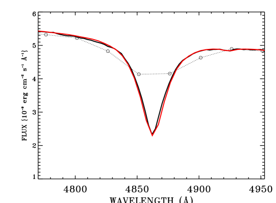
Figure 3.— The H$\beta$ spectral region. Solid line: final STIS flux, red line: Kurucz (2003) $R=500$ model scaled to $3.46\times 10^{-9}$ erg cm^-2 s^-1 at 5556 Å, dotted line with open circles: Hayes fluxes adjusted by 1.006 and wavelengths converted to vacuum to match STIS and the model.

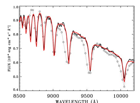
Figure 4.— As in Figure 3 for the region of the H I Paschen lines, where the Hayes (1985) spectrophotometry differs the most from STIS and the Kurucz model. At these longest wavelengths of the STIS CCD data, the de-fringing technique leaves some residuals at the $\sim$2% level. The STIS data and $R=500$ model agree within the uncertainty of the de-fringing.

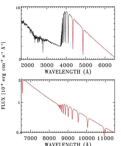
Figure 5.— Absolute flux distribution of Vega as measured by STIS below 4200 Å and as determined by the Kurucz (2003) $R=500$ model at the longer wavelengths. Below 3000 Å the spectrum is dominated by metal line blanketing, while above 3000 Å, only the Balmer and Paschen lines of hydrogen are deeper than $\sim$2% at the STIS resolution of $R=\sim 500$. The top panel shows the peak of the flux distribution down to $2\times 10^{-9}$ erg cm^-2 s^-1 Å^-1, while the lower panel covers the next factor of five lower fluxes.

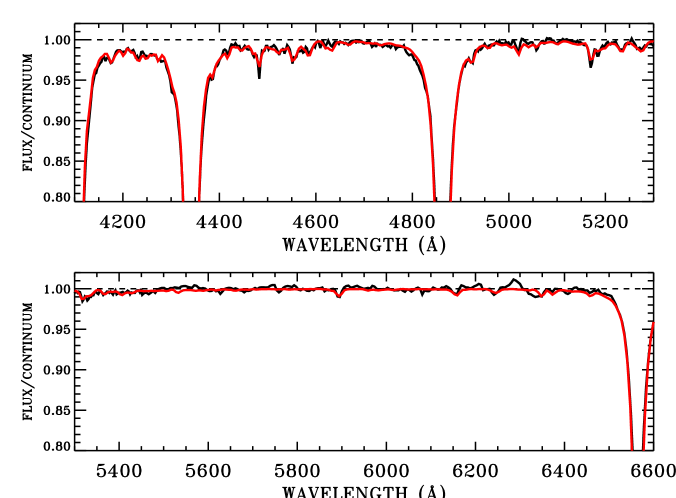
Figure 6.— Comparison of STIS (black) to the Kurucz (2003) model (red) that has effective temperature 9550 K and $\log g=3.95$ from H$\delta$ to H$\alpha$. The observations and theory agree to $\sim$1%.

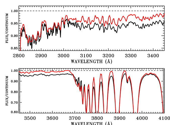
Figure 7.— Comparison as in Figure 6 for the Balmer continuum region. Systematic differences of up to $\sim$3% are prevalent. The upper panel has an expanded vertical scale in comparison to the lower panel.

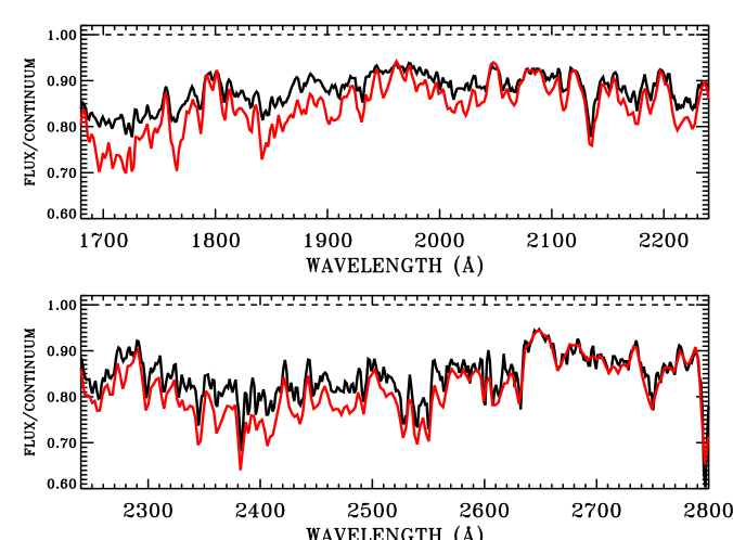
Figure 8.— Comparison in the UV below 2800 Å, where there is an excellent correlation in the wavelengths of the detailed spectral features. However, the model often shows an excess of metal line blanketing by up to several percent.

Table 1Journal of Observations

Root	Mode	Aper.	Date	Time	Propid	Exptime(s)	CR-split	Postarg
								(arcsec)
O8I105010	G230LB	52X2	03-06-30	11:00:47	9664	0.9	3	0.5
O8I105020	G230LB	52X2	03-06-30	11:03:02	9664	18.0	3	0.5
O8I105030	G230LB	52X2	03-06-30	11:08:37	9664	0.9	3	0.0
O8I105040	G230LB	52X2E1	03-06-30	11:12:38	9664	0.9	3	0.0
O8I105060	G430L	52X2	03-06-30	12:10:37	9664	0.9	3	0.0
O8I105070	G750L	52X2	03-06-30	12:17:45	9664	0.9	3	0.0
O8I106010	G430L	52X2	03-08-23	22:29:15	9664	0.9	3	0.0
O8I106020	G230LB	52X2	03-08-23	22:36:23	9664	0.9	3	0.0
O8I106030	G230LB	52X2	03-08-23	22:41:37	9664	18.0	3	0.0
O8I106040	G430L	52X2	03-08-23	22:49:00	9664	0.9	3	0.0
O8I106050	G750L	52X2	03-08-23	22:59:07	9664	1.5	5	0.0

References

- (1) Bessell, M. S., Castelli, F., & Plez, B. 1998, AA, 333, 231
- (2) Bohlin, R. C. 1996, AJ, 111, 1743
- (3) Bohlin, R. 1998, Instrument Science Report, STIS 98-01 (Baltimore: STScI)
- (4) Bohlin, R. C., Harris, A. W., Holm, A. V., & Gry, C. 1990, ApJS, 73, 413
- (5) Bohlin, R. C. 2000, AJ, 120, 437
- (6) Bohlin, R. 2003, 2002 HST Calibration Workshop, eds. S. Arribas, A. Koekemoer, and B. Whitmore (Baltimore: STScI), p. 115
- (7) Bohlin, R. C., Dickinson, M. E., & Calzetti, D. 2001, AJ, 122, 2118
- (8) Bohlin, R. & Goudfrooij, P. 2003, Instrument Science Report, STIS 03-03, (Baltimore: STScI)
- (9) Castelli, F. & Kurucz, R. L. 1994, AA, 281, 817
- (10) Cohen, M., Walker, R. G., Barlow, M. J., & Deacon, J. R. 1992, AJ, 104, 1650
- (11) Cohen, M., Wheaton, W. A., & Megeath, S. T. 2003a, AJ, 126, 1090
- (12) Cohen, M., Megeath, S. T., Hammersley, P. L., Martin-Luis, F., & Stauffer, J. 2003b, AJ, 125, 2645
- (13) Colina, L. & Bohlin, R. C. 1994, AJ, 108, 1931
- (14) Gilliland, R. L., Goudfrooij, P., & Kimble, R. A. 1999, PASP, 111, 1009 (GGK)
- (15) Gulliver, A. F., Hill, G., & Adelman, S. J. 1994, ApJL, 429, L81
- (16) Hanbury Brown, R., Davis, J., & Allen, L. R. 1974, MNRAS, 167, 121
- (17) Hayes, D. S. 1985, in Calibration of Fundamental Stellar Quantities, Proc. of IAU Symposium No. 111, eds. D. S. Hayes, L. E. Pasinetti, A. G. Davis Philip (Reidel: Dordrecht), p. 225
- (18) Hill, G., Gulliver, A.F., and Adelman, S.J. 1996, in Model Atmospheres and Spectrum Synthesis, ASP Conf 108, (eds. S.J. Adelman, F. Kupka, and W.W. Weiss) pp. 184-192
- (19) Johnson, H. L., Mitchell, R. I., Iriarte, B., & Wisniewski, W. Z. 1966, Comm. Lun. & Pl. Lab, 63 (Tucson: Univ. of Az)
- (20) Kurucz, R. L. 1995, ”The Solar Spectrum: Atlases and Line Identifications,” in Laboratory and Astronomical High Resolution Spectra, ASP Conf. Series 81, (eds. A.J. Sauval, R. Blomme, and N. Grevesse) (San Francisco: Astron. Soc. of the Pacific), pp. 17-31
- (21) Kim Quijano, J., et al. 2003, ”STIS Instrument Handbook”, Version 7.0, (Baltimore: STScI).
- (22) Kurucz, R. L. 2003, http://kurucz.harvard.edu/
- (23) Landolt, A. U. 1992, 104 340
- (24) Megessier, C. 1995, A&A, 296, 771
- (25) Seaton, M. 1979, MNRAS, 187, 73P
- (26) Strongylis, G. & Bohlin, R. C. 1979, PASP, 91, 205