Two-dimensional structure of thin transonic discs: observational manifestations

Abstract

We study the two-dimensional structure of thin transonic accretion discs in the vicinity of a non-spinning black hole within the framework of hydrodynamical version of the Grad-Shafranov equation. Our analysis focuses on the region inside the marginally stable orbit (MSO), $r<r_{\rm ms}$. We show that all components of the dynamical force in the disc become significant near the sonic surface and (especially) in the supersonic region. Under certain conditions, the disc structure can be far from radial, and we review the affected disc properties, in particular the role of the critical condition at the sonic surface. Finally, we present a simple model aimed at explaining the quasi-periodical oscillations that have been observed in the infra-red and X-ray radiation of the Galactic Centre.

1 Introduction

The investigation of accretion flows near black holes (BHs) is undoubtedly of great astrophysical interest. Substantial energy release must take place near BHs, and general relativity effects, attributable to strong gravitational fields, must show up there. Depending on external conditions, both quasi-spherical and disc accretion flows can be realized. The structure of thin accretion discs has been the subject of many papers. Many results were included in textbooks [1, 2]. Lynden-Bell [3] was the first to point out that supermassive BHs surrounded by accretion discs could exist in galactic nuclei. Subsequently, a theory for such discs was developed that is now called the standard model, or the model of the $\alpha-$disc [4, 5, 6].

Since then the standard disc thickness prescription has been widely used,

$$H\approx r\frac{c_{\rm s}}{v_{\rm K}},$$ (1)

where the disc thickness $H$ is assumed to be determined by the balance of gravitational and accreting matter pressure forces with the dynamical force neglected. This relation was later used in the renowned approach where all quantities were averaged over the disc thickness [7], with a lot of such one-dimensional models following [8, 9, 10, 11, 12, 13, 14, 15, 16, 17]. As for the two-dimensional structure of accretion discs, it was investigated mostly only numerically and only for thick discs [9, 18, 19, 20].

Even though standard disc thickness prescription (1) and the averaging procedure are likely to be valid in the region of stable orbits $r>r_{\rm ms}$ [1], they in our view require a more serious analysis. It is the assumption that the transverse velocity $v_{\theta}$ may always be neglected in thin accretion discs all the way up to horizon [21], i.e. that the disc thickness is always determined by (1), that is the most debatable [22]. This assumption is widely used, explicitly or implicitly, virtually in all papers devoted to thin accretion discs [23, 24].

There is a brief discussion on thin discs in this volume that covers theory shortcomings and a brief description of our approach (cf. Sec. named Thin disk in [22]). In this paper we briefly describe our study of subsonic and transonic regions of thin discs followed in Sec. 5 by the elaborate discussion of the supersonic flow. Finally, in Sec. 6 we develop a toy model for explaining the observed quasi-periodical oscillations detected in the infra-red and X-ray observations of the GC.

2 Basic equations

We consider thin disc accretion on to a BH in the region where there are no stable circular orbits. The contribution of viscosity should no longer be significant here [22]. Hence we may assume that an ideal hydrodynamics approach is suitable well enough for describing the flow structure in this inner area of the accretion disc. Below, unless specifically stated, we consider the case of non-spinning BH, i.e. use the Schwarzschild metric, and use a system of units with $c=G=1.$ We measure radial distances in the units of $M$, the BH mass.

In Boyer-Lindquist coordinates the Schwarzschild metric is [25]

$${\rm d}s^{2}=-\alpha^{2}{\rm d}t^{2}+g_{ik}{\rm d}x^{i}{\rm d}x^{k},$$ (2)

where

$$\alpha^{2}=1-2/r,\quad g_{rr}=\alpha^{-2},\quad g_{\theta\theta}=r^{2},\quad g_{\varphi\varphi}=\varpi^{2}=r^{2}\sin^{2}\theta.$$ (3)

We reduce our discussion to the case of axisymmetric stationary flows. For an ideal flow there are three integrals of motion conserved along the streamlines, namely entropy, $S$, energy $E=\mu\alpha\gamma$, and $z$-component of angular momentum $L=\mu\varpi u_{\hat{\varphi}}$, where $\mu=(\rho_{m}+P)/n$ ($\rho_{m}$ is internal energy density, $P=nT$ is pressure) is relativistic enthalpy. The relativistic Bernoulli equation $u^{2}_{\rm\hat{p}}=\gamma^{2}-u_{\hat{\varphi}}^{2}-1$, where $u_{\rm\hat{p}}$ is the physical poloidal $4$-velocity component [22, 26, 27], now becomes

$$u^{2}_{\rm\hat{p}} =\frac{E^{2}-\alpha^{2}L^{2}/\varpi^{2}-\alpha^{2}\mu^{2}}{\alpha^{2}\mu^{2}}.$$ (4)

Below we use another angular variable $\Theta=\pi/2-\theta$ and for the sake of simplification we adopt the polytropic equation of state $P=k(S)n^{\Gamma}$ so that temperature and sound velocity can be written as [1]

$$T=k(S)n^{\Gamma-1};\qquad c^{2}_{\rm s}=\frac{\Gamma}{\mu}k(S)n^{\Gamma-1}.$$ (5)

3 Subsonic flow

Following Sec. 1, we assume that the $\alpha$-disc theory holds outside the MSO. We adopt the flow velocity components, which this theory yields on the MSO $r=r_{\rm ms},$ as the first three boundary conditions for our problem. For the sake of simplicity we consider the radial velocity, which is responsible for the inflow, to be constant at the surface $r=r_{\rm ms}$ and equal to $u_{0}$ and the toroidal velocity to be exactly equal to that of a free particle revolving at $r=r_{\rm ms}$. We also assume the speed of sound to be constant at the MSO, $c_{\rm s}=c_{0}=\mathrm{const}$. Having introduced $\Theta_{\rm ms}$ [27] — the Lagrange coordinate of streamlines at the MSO — for $c_{\rm s}\ll 1$, i.e. non-relativistic temperature, we obtain from (4) and (5),

$$u^{2}_{\rm\hat{p}}=u_{0}^{2}+w^{2}+\frac{2}{\Gamma-1}\left(c_{0}^{2}-c^{2}_{\rm s}\right)+\frac{1}{3}\left(\Theta^{2}_{\rm ms}-\Theta^{2}\right)+\dots$$ (6)

The quantity

$$w^{2}(r)=\frac{e_{0}^{2}-\alpha^{2}l_{0}^{2}/r^{2}-\alpha^{2}}{\alpha^{2}}\equiv\frac{1}{\alpha^{2}}\frac{(6-r)^{3}}{9r^{3}},$$ (7)

where $e_{0}=E_{0}/\mu_{0}$ and $l_{0}=L/(\mu_{0}\cos\Theta_{\rm ms})$, is the poloidal four-velocity of a free particle having zero poloidal velocity at the MSO.

In the extreme subsonic case, $u_{\rm\hat{p}}\ll c_{\rm s}$, the Grad-Shafranov hydrodynamic equation is significantly simplified [22, 27]. The numerical results are shown in Fig. 2. In the subsonic region, $r_{*}<r\leq r_{\rm ms}\equiv 3r_{\rm g}$, the disc thickness rapidly diminishes, and at the sonic surface we have $H(r_{*})=u_{0}/c_{0}H(r_{\rm ms})$, so that you cannot neglect the dynamical force there.

We stress that taking the dynamical force into account is indeed extremely important. This is because, unlike zero-order standard disc thickness prescription (1), the Grad-Shafranov equation has second order derivatives, i.e. contains two additional degrees of freedom. This means that the critical condition only fixes one of these degrees of freedom (e.g. imposes some limitations on the form of the flow) rather than determines the angular momentum of the accreting matter [22, 27].

4 Transonic flow

In order to verify our conclusions we consider the flow structure in the vicinity of the sonic surface in more detail. Since the smooth transonic flow is analytical at a singular point $r=r_{*},\Theta=0$ [28], it is possible to express the quantities via a series of powers of $h=(r-r_{*})/r_{*}$ and $\Theta$. Substituting these expansions into equations of motion we get a set of equations on the coefficients which allows us to reconstruct the flow structure in the vicinity of the sonic point (see Fig. 2), in particular

$$u^{2}_{\rm\hat{p}} =c_{*}^{2}\left[1-2\eta_{1}h+\frac{1}{6}(\Gamma-1)\,\frac{a_{0}^{2}}{c_{0}^{2}}\Theta^{2}+\frac{2}{3}(\Gamma+1)\eta_{1}^{2}\Theta^{2}\right],$$

$$c^{2}_{\rm s} =c_{*}^{2}\biggl{[}1+\left(\Gamma-1\right)\eta_{1}h+\frac{1}{6}(\Gamma-1)\,\frac{a_{0}^{2}}{c_{0}^{2}}\Theta^{2}-\frac{1}{3}(\Gamma-1)(\Gamma+1)\eta_{1}^{2}\Theta^{2}\biggr{]},$$ (8)

where $a_{0}=\left[2/(\Gamma+1)\right]^{(\Gamma+1)/2(\Gamma-1)}c_{0}/u_{0}$ gives the compression of streamlines, $a_{0}=H(r_{\rm ms})/H(r_{*})$, and $\eta_{1}\sim u_{0}^{-1}$. Equation (8) yields shape of the sonic surface, $u_{\rm\hat{p}}=c_{\rm s}$; it has the standard parabolic form $h=(\Gamma+1)\eta_{1}\Theta^{2}/3$.

Since the transonic flow in the form of a nozzle (see Fig. 2) has longitudinal and transversal scales of one order of magnitude [28], near the sonic surface we have $\delta r_{\parallel}\approx\delta r_{\bot},$ i.e. $\delta r_{\parallel}\approx H(r_{*})$. Hence for thin discs (i.e. for $c_{0}\ll 1$) this longitudinal scale is always much smaller than the distance from the BH, $\delta r_{\parallel}/r_{*}\approx H(r_{*})/r_{*}\ll 1$. Only by taking the transversal velocity into account do we retain the small longitudinal scale $\delta r_{\parallel}\ll r_{\rm g}.$ This scale is left out during the standard one-dimensional approach.

5 Supersonic flow

Since the pressure gradient becomes insignificant in the supersonic region, the matter moves here along the trajectories of free particles. Neglecting the $\nabla_{\theta}P$ term in the $\theta$-component of relativistic Euler equation [29], we have [21]

$$\alpha u_{\hat{r}}\frac{\partial(ru_{\hat{\Theta}})}{\partial r}+\frac{(ru_{\hat{\Theta}})}{r^{2}}\frac{\partial(ru_{\hat{\Theta}})}{\partial\Theta}+(u_{\hat{\varphi}})^{2}\tan\Theta=0.$$ (9)

Here, using the conservation law of angular momentum, $u_{\hat{\varphi}}$ can be easily expressed in terms of radius: $u_{\hat{\varphi}}=2\sqrt{3}/r$. We also introduce dimensionless functions $f(r)$ and $g(r)$: $\Theta f(r)=ru_{\hat{\Theta}}$ and $g(r)=-\alpha u_{\hat{r}}>0$. Using (9) and the definitions above, we obtain an ordinary differential equation for $f(r)$ which could be solved if we knew $g(r)$:

$$\frac{{\rm d}f}{{\rm d}r}=\frac{f^{2}+12}{r^{2}g(r)}.$$ (10)

From (4) we have $u^{2}_{\rm\hat{p}}\rightarrow w^{2}$ as $r\rightarrow r_{\rm g}$. On the other hand, $u_{\rm\hat{p}}\approx c_{*}\approx c_{0}$ for $r\lesssim r_{*}$. Therefore, the following approximation should be valid throughout the $r_{\rm g}<r<r_{*}$ region, $g(r)\approx\sqrt{(\alpha w)^{2}+(\alpha c_{*})^{2}}$.

Equation (10) governs the supersonic flow structure for the case of non-spinning BH. To get a better match with observations (cf. Sec. 6), we also consider a more general case of spinning BH, i.e. a Kerr BH with non-zero specific angular momentum $a$. After some calculation, equation (10) can be generalized to the Kerr metric with a strikingly simple form,

$$\frac{{\rm d}f}{{\rm d}r}=\frac{f^{2}+a^{2}\left(1-e_{0}^{2}\right)+l_{0}^{2}}{r^{2}\tilde{g}\left(r\right)},$$ (11)

where $\tilde{g}\left(r\right)$ is a straightforward generalization of $g(r)$ to the Kerr case; we omit it here due to space limitations. For the Schwarzschild BH ($a=0$, $e_{0}=\sqrt{8/9}$, $l_{0}=2\sqrt{3}$ [28]) equation (11) reduces back to (10).

Integrating (11), we obtain

$$f\left(r\right)=\kappa\tan\left[\kappa\int_{r_{*}}^{r}\frac{d\xi}{\xi^{2}g(\xi)}+\frac{\pi}{2}\right],$$ (12)

where $\kappa=\sqrt{a^{2}\left(1-e_{0}^{2}\right)+l_{0}^{2}}$ and $\pi/2$ has been to a good accuracy substituted for the integration constant $\arctan\left[f(r_{*})/\sqrt{3}\right]$.

The results of numerical calculations are presented in Fig. 2.

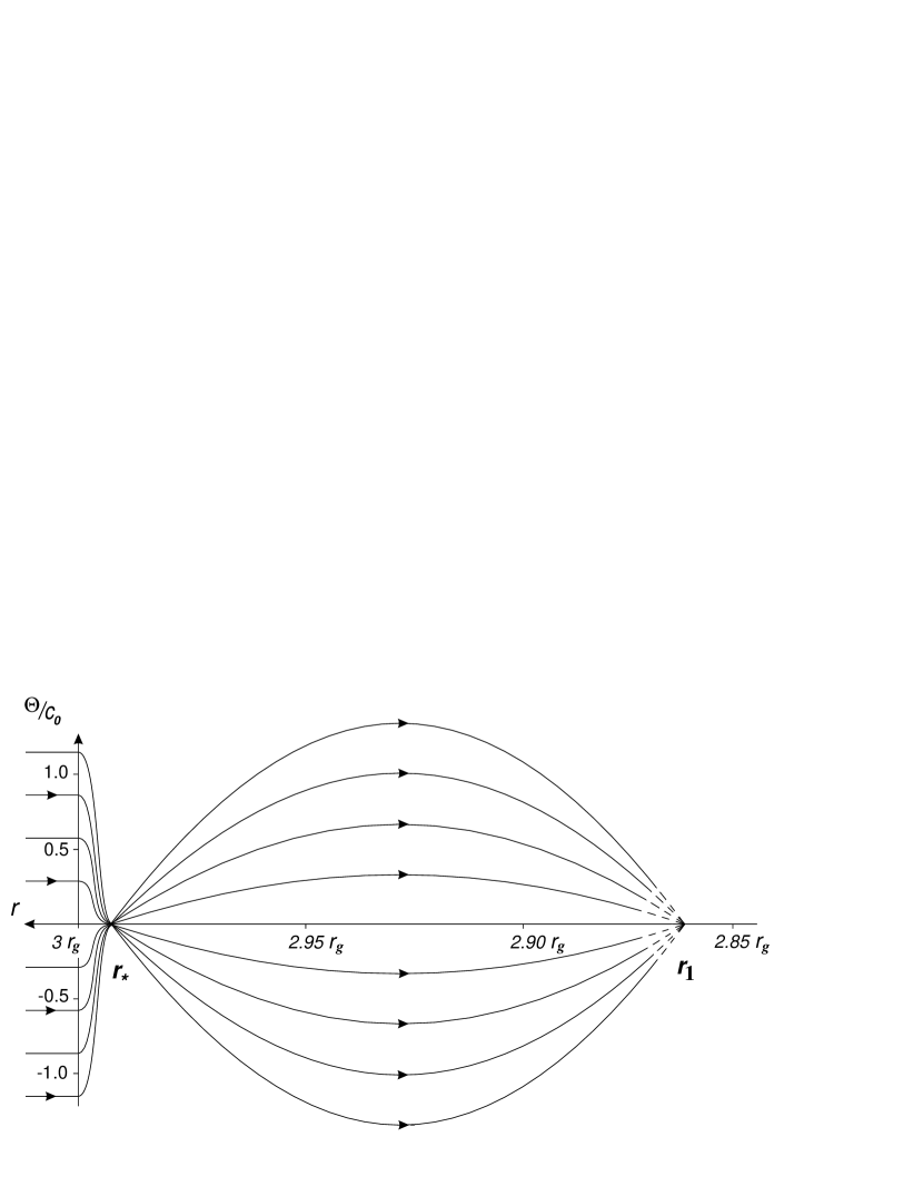
Figure 1: The structure of a thin accretion disc (actual scale) for $c_{0}=10^{-2}$, $u_{0}=10^{-5}$ after passing the MSO $r=3r_{\rm g}$ ($a=0$, Schwarzschild case). As sufficient dissipation can take place in the vicinity of the first node $r=r_{\rm 1}$, we do not prolong the flow lines to the region $r<r_{\rm 1}$.

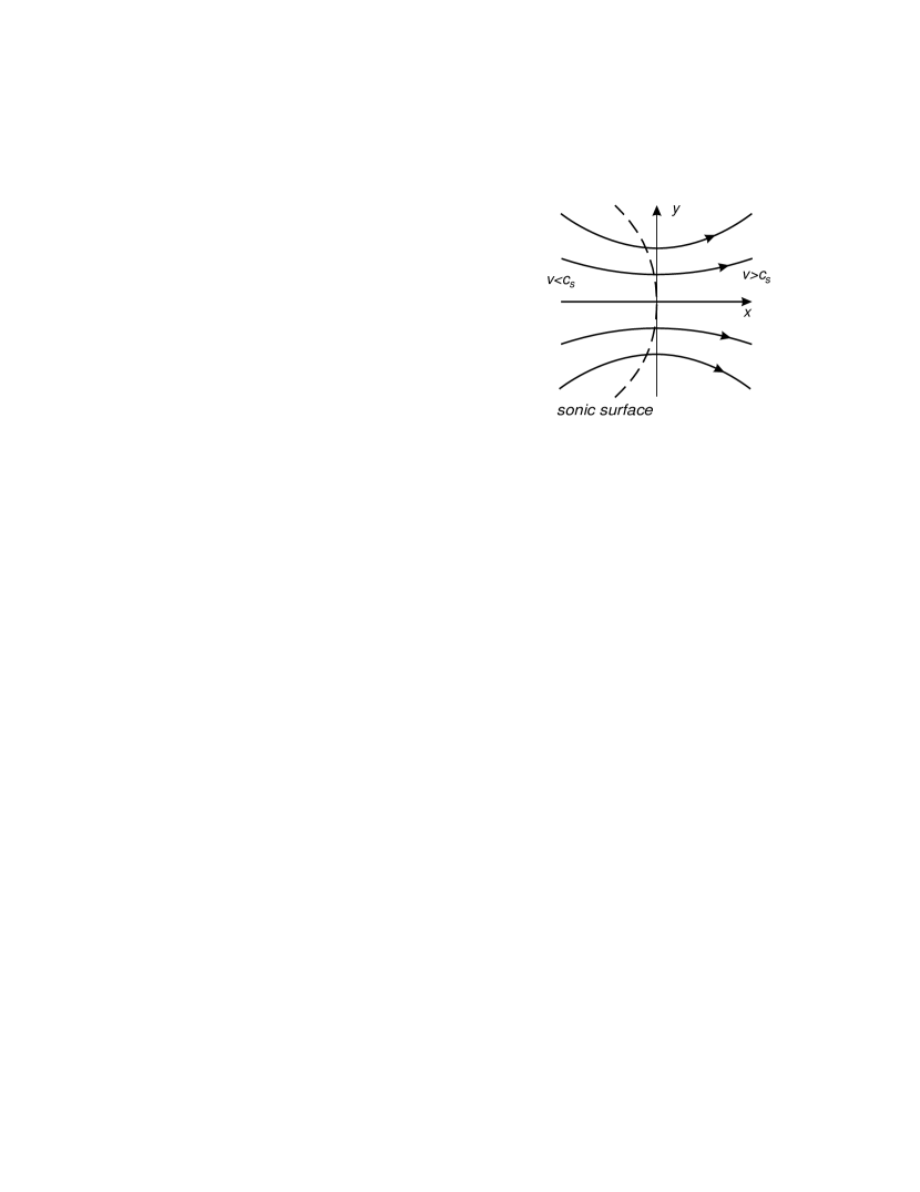
Figure 2: Schematics of thin disc streamlines profile around the sonic point. The flow has the form of the standard nozzle. Here $x=-h$, and $y=\Theta$.

In the supersonic region the flow performs transversal oscillations about the equatorial plane, their frequency independent of their amplitude. We see as well that the maximum thickness of the disc in the supersonic (and, hence, ballistic) region, which is controlled by the transverse component of the gravitational force, actually coincides with the disc thickness within the stable orbits region, $r>r_{\rm ms}$, where standard estimate (1) is correct.

Once diverged, the flow converges once again at a ‘nodal’ point closer to the BH. The radial positions the nodes are given by the implicit formula $f(r_{n})=\pm\infty,$ i.e.

$$\kappa\int_{r_{n}}^{r_{*}}\frac{d\xi}{\xi^{2}g(\xi)}=n\pi,$$ (13)

where $n$ is the node number; the node with $n=0$ corresponds to the sonic surface. In this formula the sonic radius $r_{*}\equiv r_{0}$ can be to a good accuracy approximated by $r_{\rm ms}=r_{\rm ms}(a)$ the expression for which can be found in most textbooks [1]. Figure 4 shows the positions of nodes for different values of $c_{0}$ (the positions do not depend on $u_{0}$ for $u_{0}\ll c_{0}$) and the BH spin parameter $a$.

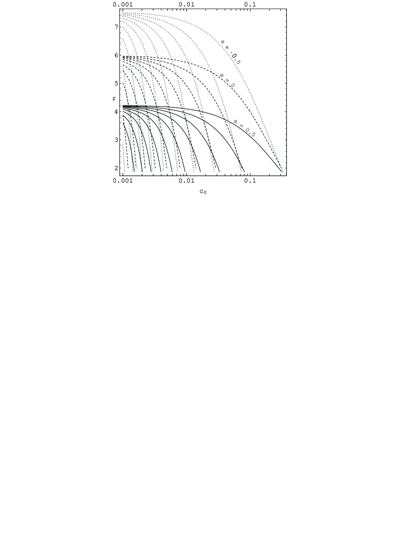
Figure 3: Radial positions (in the units of $M$) of the nodes for a range of initial sound velocities. Dotted, dashed, and solid curves correspond to the cases $a=-0.5$, $a=0$, and $a=0.5$ respectively. Each curve relates the radial position of a node to a value of the initial sound velocity. Intersection points of these curves with the line $c_{0}={\rm const}$ give the the nodes’ radial positions for that particular value of $c_{0}$.

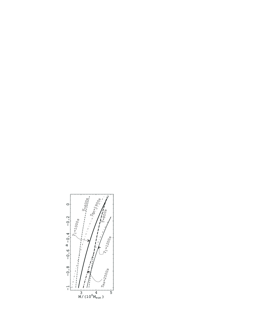
Figure 4: Relation of $a$ vs. $M$. Dashed, dash-dotted, and solid lines come from matching $\overline{T}$ ($700\pm 100$ s), $T_{\rm ms}$ ($2200\pm 300$ s), and $T_{0}$ ($1100\pm 100$ s) respectively. The resulting error polygon is bolded.

The matter travel time between the nodes has weak dependence not only on $u_{0}$ but also on $c_{0}$ as well. This provides a means for testing the theory via observations, and we do this in the following section.

6 Applications to observations

Suppose some perturbation in the disc (a “chunk”) approaches the MSO. We expect to observe radiation coming from the chunk with the period of its orbital motion,

$$T_{\rm ms}\left(a\right)=2\pi\left(r^{3/2}_{\rm ms}+a\right),$$ (14)

where $a$ is the angular momentum per unit mass of the BH and $r_{\rm ms}$ is an estimate of the distance from the BH to the chunk [1]. After a number of rotations, the chunk reaches the MSO and passes through the nodal structure derived earlier (cf. Sec. 5) generating a flare. Each time the chunk passes through a node, it generates some additional radiation, and therefore the flare is likely to consist of several peaks. We believe that it is these peaks that were discovered in the infra-red and X-ray observations of the GC [30, 31].

The time interval between the detection of two subsequent peaks equals the time it takes for the chunk to pass between two adjacent nodes ($n$-th and $(n-1)$-th), $T_{n}^{(1)}$, plus the difference in travel times to the observer for the radiation coming from the $n$-th and $(n-1)$-th nodes, $T_{n}^{(2)}$:

$$T_{n}=T_{n}^{(1)}+T_{n}^{(2)},$$ (15)

where $n$ is the index of the observed time interval (counting from one).

The first term in r.h.s. of (15) can be easily obtained from the analysis of particle’s geodesics in the equatorial plane [1]

$$T_{n}^{(1)}\left(a,c_{\rm s}\right)=\int_{r_{n}}^{r_{n-1}}\frac{u^{t}}{u^{r}}{\rm d}r=\int_{r_{n}}^{r_{n-1}}\frac{\left(-e_{0}g^{tt}+l_{0}g^{t\varphi}\right)|_{\theta=\pi/2}}{g\left(r\right)}{\rm d}r,$$ (16)

where the coefficients of the inverse metric are $g^{tt}=-\Sigma^{2}/(\rho^{2}\Delta)$ and $g^{t\varphi}=\omega g^{tt}$; the definitions of $\Sigma$, $\rho$, $\Delta$, and $\omega$ can be found elsewhere in this volume [22].

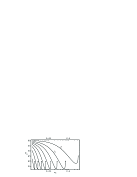
Figure 5: The dependence of time intervals between the peaks in a flare on the speed of sound in the disc, $c_{0}$, for a moderately spinning BH ($a=-0.5$). The uppermost curve corresponds to the time interval $T_{1}$ between the the $0$th and $1$st peaks, the second curve from the top corresponds to the time interval $T_{2}$ between the $1$st and $2$nd ones, etc. All intervals $T_{n}$ behave very similarly: they first decrease with $c_{0}$ and then abruptly increase to infinity due to time dilation when the innermost node in the pair comes close to the BH horizon (which is indicated with upward arrows). Even though individual time intervals between subsequent peaks in the flare may depend on the temperature in the disc (which is proportional to $c_{0}^{2}$, see (5)), their minimum and maximum values remain the same for the range of sound velocities where there are several intervals observed. In the particular case of $a=-0.5$, illustrated in the figure, we have $T_{\rm min}\approx 32$ and $T_{\rm max}\approx 60$ with all other time intervals lying in between.

For definiteness and simplicity, we assume that the observer is located along the rotation axis of the BH. On its way to the observer, the radiation travels along the null geodesic that originates at a node in the equatorial plane (e.g. $r=r_{n}$, $\theta=\pi/2$) and reaches the observer at infinity ($r=\infty$, $\theta=0$). Using these as boundary conditions for null geodesics in the Kerr metric [32], we numerically find $T_{n}^{(2)}(a,c_{\rm s})$.

Figure 5 shows the dependence of observed time intervals on the value of the speed of sound in the disc. Although each individual time interval may depend on $c_{0}$, the range [$T_{\rm min}(a)$, $T_{\rm max}(a)$] of observed time intervals (see the caption to Fig. 5) is independent of $c_{0}$. With such weak dependence on the speed of sound in the disc, we have only two matching parameters: the specific spin $a$ and the mass $M$ of the BH.

In the flare precursor section we associate the period $T_{\rm ms}$ with the $2200\pm 300$ s one (group 5, cf. Table 2 in [30]) and the time interval $T_{1}$ with the period of $1100\pm 100$ s (group 4 in [30]). In consistency with the infra-red observations of the flare, the periods $T_{1}$, $T_{2}$, etc. chirp with the peak number [31], i.e. resemble the QPO structure and thus form a cumulative peak of a larger width shifted to higher frequencies on the flares’ power density spectra ($700\pm 100$ s, group 3, cf. Fig. 3a and 4a in [30]). We can estimate the average frequency of this peak as $1/\overline{T}=1/2\left(1/T_{\rm min}+1/T_{\rm max}\right)$. The results of the periods’ matching procedure are shown in Fig. 4. Despite large uncertainties in the observational data allowing significant freedom of $a$ and $M$, high positive values of $a$ (i.e. the disc orbiting in the same direction as the BH spin) are clearly ruled out.

References

- [1] Shapiro S.L., Teukolsky S.A., Black Holes, White Dwarfs, and Neutron Stars (Wiley–Interscience Publication, New York, 1983).
- [2] Lipunov V.M., Astrophysics of Neutron Stars (Springer-Verlag, Berlin, 1992).
- [3] Lynden-Bell D., Nature 223, 690 (1969).
- [4] Shakura N.I., AZh 49, 921 (1972).
- [5] Shakura N.I., Sunyaev R.A., A&A 24, 337 (1973).
- [6] Novikov I.D., Thorne K.S. Black Holes (C. DeWitt, B. DeWitt., eds, Gordon and Breach, New York, 1973).
- [7] Paczyński B., Bisnovatyi-Kogan G.S., Acta Astron. 31, 283 (1981).
- [8] Abramowicz M.A., Czerny B., Lasota J.-P., Szuszkiewicz E., ApJ 332, 646 (1988).
- [9] Papaloizou J., Szuszkiewicz E., MNRAS 268, 29 (1994).
- [10] Riffert H., Herold H., ApJ 450, 508 (1995).
- [11] Chen X., Abramowicz M.A., Lasota J.-P., ApJ 476, 61 (1997).
- [12] Narayan R., Kato S., Honma F., ApJ 476, 49 (1997).
- [13] Peitz J., Appl S., MNRAS 286, 681 (1997).
- [14] Beloborodov A.M., MNRAS 297, 739 (1998).
- [15] Gammie C.F., Popham R., ApJ 498, 313 (1998).
- [16] Gammie C.F., Popham R., ApJ 504, 419 (1998).
- [17] Artemova Yu.V., Bisnovatyi-Kogan G.S., Igumenshchev I.V., Novikov I.D., ApJ 549, 1050 (2001).
- [18] Igumenshchev I.V., Beloborodov A.M., MNRAS 284, 767 (1997).
- [19] Balbus S.A., Hawley J.F., Rev. Mod. Phys. 70, 1 (1998).
- [20] Krolik J.H., Hawley J.F., ApJ 573, 754 (2002).
- [21] Abramowicz M.A., Lanza A., Percival M.J., ApJ 479, 179 (1997).
- [22] Beskin V.S., this volume (2004).
- [23] Abramowicz M.A., Zurek W., ApJ 246, 314 (1981).
- [24] Chakrabarti S., ApJ 471, 237 (1996).
- [25] Landau L.D., Lifshits E.M., The Classical Theory of Fields (4th edn. Butterworth-Heinemann, 1987).
- [26] Beskin V.S., Phys. Usp. 40, 659 (1997).
- [27] Beskin V.S., Kompaneetz R.Yu., Tchekhovskoy A.D., Astron. Lett. 28, 543 (2002).
- [28] Landau L.D., Lifshits E.M., Fluid mechanics (2nd edn. Butterworth-Heinemann, 1987).
- [29] Frolov V.P., Novikov I.D., Black Hole Physics (Kluwer Academic Publishers, Dordrecht, 1998).
- [30] Ashenbach B., Grosso N., D. Porquet, and Predehl P., A&A, accepted, astro-ph/0401589 (2004).
- [31] Genzel R., Schödel R., Ott T. et al., Nature 425, 934 (2003).
- [32] Carter B., Phys. Rev. 174, 5 (1968).
- [33] Beskin V.S., Pariev V.I., Phys. Usp. 36, 529 (1993).
- [34] Bondi H., MNRAS 112, 195 (1952).
- [35] Igumenshchev I.V., Abramowicz M.A., Narayan R., ApJ 537, L27 (2000).
- [36] Paczyński B., Wiita P.J., A&A 88, 23 (1980).
- [37] Thorne K.S., Price R.N., Macdonald D.A., Black Holes: The Membrane Paradigm (Yale Univ. Press, New Haven, CT, 1986).