Observable primordial vector modes

Abstract

Primordial vector modes describe vortical fluid perturbations in the early universe. A regular solution exists with constant non-zero radiation vorticities on super-horizon scales. Baryons are tightly coupled to the photons, and the baryon velocity only decays by an order unity factor by recombination, leading to an observable CMB anisotropy signature via the Doppler effect. There is also a large B-mode CMB polarization signal, with significant power on scales larger than $l\sim 2000$. This B-mode signature is distinct from that expected from tensor modes or gravitational lensing, and makes a primordial vector to scalar mode power ratio $\sim 10^{-6}$ detectable. Future observations aimed at detecting large scale $B$-modes from gravitational waves will also be sensitive to regular vector modes at around this level.

Observations of the cosmic microwave background (CMB) show that the primordial perturbation was almost certainly dominated by adiabatic scalar (density) modes. However it is well known that there are several possible scalar isocurvature modes Bucher et al. (2001) that could be present at some level. In the presence of a primordial magnetic field, there is also an observable vector mode perturbation Subramanian et al. (2003); Lewis (2004) sourced by the anisotropic stress of the magnetic field. Other sources such as topological defects can also source vector modes. Here we concentrate on the rarely-considered regular primordial (unsourced) vector modes, which are non-decaying solutions of the perturbation equations in the presence of free streaming neutrinos Rebhan (1992). We show that a very small primordial regular vector mode amplitude could be observable.

In the absence of an initial large scale radiation vorticity the vector modes remain in a decaying mode and have essentially no observational signature. They are therefore not predicted to be present at any significant level in inflation or other simple models. However there is a regular mode with a non-zero initial photon vorticity, having equal and opposite initial photon and neutrino angular momenta such that the total large scale angular momentum is zero. This is the vector analogue of the scalar neutrino isocurvature velocity mode discussed in Ref. Bucher et al. (2001), and constitutes a valid possible component of the general primordial perturbation. These velocity modes would have to be excited after neutrino decoupling and are hence difficult to produce and somewhat contrived. But they remain a logical possibility that can be constrained by observation, and if observed would be a powerful way to rule out most theoretical models (for constraints on the scalar mode see e.g. Ref. Bucher et al. (2004) and references therein). The vector mode can be detected at very small amplitudes and distinguished from the various scalar modes because of its distinct non-zero $B$-mode (curl-like) CMB polarization signal that is absent with only linear scalar modes.

As we show, the vector $B$-mode signature is quite different from that expected from weak lensing or primordial tensor modes. On large scales the spectrum is similar to that from tensors, so observations aimed at detecting the $B$-modes from primordial tensors will also be sensitive to the large scale part of the vector power spectrum, but they can easily be distinguished by the vector mode power on smaller scales. The physical difference between the spectra is that tensor modes rapidly decay as soon as they come inside the horizon, whereas the vortical modes are nearly constant during radiation domination, decaying only on small scales though damping towards the end of tight coupling.

Even more contrived regular modes exist with non-zero primordial neutrino octopole (or higher) Rebhan (1992); Rebhan and Schwarz (1994), however these have a much weaker observational signature and are not considered further here.

.1 Covariant Equations

We consider linear perturbations in a flat FRW universe evolving according to general relativity with a cosmological constant, neglect any velocity dispersion of the dark matter and baryon components, and approximate the neutrinos as massless. Perturbations can be described covariantly in terms of a 3+1 decomposition with respect to some choice of observer velocity $u_{a}$ (we use natural units, and the signature where $u_{a}u^{a}=1$), following Refs. Ellis et al. (1983); Gebbie and Ellis (2000); Challinor and Lasenby (1999). Projected spatial derivatives orthogonal to $u_{a}$ can be used to quantify perturbations to scalar quantities, for example the pressure perturbation can be described in terms of ${\mathrm{D}}_{a}p$ where the spatial derivative is

$${\mathrm{D}}_{a}\equiv\nabla_{a}-u_{a}u^{b}\nabla_{b}.$$ (1)

Conservation of total stress-energy $\nabla^{a}T_{ab}=0$ implies an evolution equation for the total heat flux $q_{a}$

$$\dot{q}_{a}+\frac{4}{3}\Theta q_{a}+(\rho+p)A_{a}-{\mathrm{D}}_{a}p+{\mathrm{D}}^{b}\pi_{ab}=0.$$ (2)

where $\rho$ is the energy density, $\dot{q}_{a}\equiv u^{b}\nabla_{b}q_{a}$, $\Theta\equiv\nabla^{a}u_{a}$ is three times the Hubble expansion, $A_{a}\equiv u_{b}\nabla^{b}u_{a}$ is the acceleration, and $\pi_{ab}\equiv T_{\langle ab\rangle}$ is the total anisotropic stress. Angle brackets around indices denote the projected symmetric trace-tree part (orthogonal to $u_{a}$).

We define the vorticity vector $\Omega_{a}\equiv\,\mbox{curl}\,u_{a}$ where for a general tensor

$$\,\mbox{curl}\,X_{a_{1}\dots a_{l}}\equiv\eta_{bcd(a_{1}}u^{b}{\mathrm{D}}^{c}X^{d}{}_{a_{2}\dots a_{l})}$$ (3)

and round brackets denote symmetrization. It has the evolution equation

$$\dot{\Omega}_{a}+\frac{2}{3}\Theta\Omega_{a}=\,\mbox{curl}\,A_{a}$$ (4)

and is transverse ${\mathrm{D}}^{a}\Omega_{a}=0$. Remaining quantities we shall need are the ‘electric’ $E_{ab}$ and ‘magnetic’ $H_{ab}$ parts of the Weyl tensor $C_{abcd}$

$$E_{ab}\equiv C_{acbd}u^{c}u^{d}\quad\quad H_{ab}\equiv\frac{1}{2}\eta_{acdf}C_{be}{}^{cd}u^{e}u^{f}$$ (5)

(which are frame invariant) and the shear $\sigma_{ab}\equiv{\mathrm{D}}_{\langle a}u_{b\rangle}$. The Einstein equation and the Bianchi identity give the constraint equations

$${\mathrm{D}}^{a}\sigma_{ab}-\frac{1}{2}\,\mbox{curl}\,\Omega_{b}-{\frac{2}{3}}{\mathrm{D}}_{b}\Theta-\kappa q_{b}=0$$

$${\mathrm{D}}^{a}E_{ab}-\kappa\left({\frac{\Theta}{3}}q_{b}+{\frac{1}{3}}{\mathrm{D}}_{b}\rho+{\frac{1}{2}}{\mathrm{D}}^{a}\pi_{ab}\right)=0$$

$${\mathrm{D}}^{a}H_{ab}-{\frac{1}{2}}\kappa[(\rho+p)\Omega_{b}+\,\mbox{curl}\,q_{b}]=0$$

$$H_{ab}-\,\mbox{curl}\,\sigma_{ab}+\frac{1}{2}{\mathrm{D}}_{\langle a}\Omega_{b\rangle}=0,$$ (6)

and the evolution equations

$$\dot{\sigma}_{ab}+\frac{2}{3}\Theta\sigma_{ab} = -E_{ab}-{\frac{1}{2}}\kappa\pi_{ab}$$

$$\dot{E}_{ab}+\Theta E_{ab} = \,\mbox{curl}\,H_{ab}+{\frac{\kappa}{2}}\left[\dot{\pi}_{ab}-(\rho+p)\sigma_{ab}+{\frac{\Theta}{3}}\pi_{ab}\right]$$

$$\dot{H}_{ab}+\Theta H_{ab} = -\,\mbox{curl}\,E_{ab}-{\frac{\kappa}{2}}\,\mbox{curl}\,\pi_{ab}.$$ (7)

We use natural units where $c=1$ and define $\kappa\equiv 8\pi G$.

A vector like $A_{a}$ may be split into a scalar part $A_{a}^{(0)}$ and a vector part $A_{a}^{(1)}$ where $A_{a}=A_{a}^{(0)}+A_{a}^{(1)}$, $A_{a}^{(0)}={\mathrm{D}}_{a}A$ for some first order scalar $A$ and the vector part is solenoidal $D^{a}A_{a}^{(1)}=0$. This extends to a tensor where the vector part is given by $\sigma_{ab}^{(1)}={\mathrm{D}}_{\langle a}\Sigma_{b\rangle}$ for some first order solenoidal vector $\Sigma_{b}$.

We can choose $u_{a}$ to simplify the analysis. At linear order one can always write $u_{a}=u_{a}^{\perp}+v_{a}$, where $u_{a}^{\perp}$ is hypersurface orthogonal and $v_{a}$ is first order, so $\,\mbox{curl}\,u_{a}=\,\mbox{curl}\,v_{a}$. For a zero order scalar quantity $X$ it follows that ${\mathrm{D}}_{a}X={\mathrm{D}}_{a}^{\perp}X-v_{a}\dot{X}$. For vector modes $({\mathrm{D}}_{a}^{\perp}X)^{(1)}=0$, and it is convenient to choose the frame $u_{a}$ to be hypersurface orthogonal so that $\,\mbox{curl}\,u_{a}=0$ and hence $(\bar{{\mathrm{D}}}_{a}X)^{(1)}=0$, where the bar denotes evaluation in the zero vorticity frame. From its propagation equation, vanishing of the vorticity also implies that $\bar{A}_{a}^{(1)}=0$, so the zero vorticity frame coincides with the synchronous gauge. The CDM velocity is also zero in this frame modulo a mode which decays as $1/S$ where $S$ is the scale factor.

It is convenient to expand the vector components in terms of transverse eigenfunctions of the zero order Laplacian, $Q^{\pm}_{a}$ where $S^{2}{\mathrm{D}}^{2}Q_{a}^{\pm}=k^{2}Q_{a}^{\pm}$ and $\pm$ denotes the parity. A rank-$\ell$ tensor may be expanded in terms of rank-$\ell$ eigenfunctions $Q^{\pm}_{A_{l}}$ defined by

$$Q_{A_{l}}^{\pm}\equiv\left(\frac{S}{k}\right)^{l-1}{\mathrm{D}}_{\langle a_{1}}\dots\mathrm{D}_{a_{l-1}}Q_{a_{l}\rangle}^{\pm}$$ (8)

which satisfy

$${\mathrm{D}}^{a_{l}}Q^{\pm}_{A_{l-1}a_{l}} = \frac{k}{S}\frac{(l^{2}-1)}{l(2l-1)}Q_{A_{l-1}}^{\pm}$$ (9)

$$\,\mbox{curl}\,Q_{A_{l}}^{\pm} = \frac{1}{l}\frac{k}{S}Q^{\mp}_{A_{l}}.$$ (10)

Harmonic coefficients are defined by

$$\sigma_{ab}^{(1)} = \sum\frac{k}{S}\sigma Q^{\pm}_{ab}\quad\quad H_{ab}^{(1)}=\sum\frac{k^{2}}{S^{2}}HQ^{\pm}_{ab}$$

$$q_{a}^{(1)} = \sum qQ_{a}^{\pm}\quad\quad\Omega_{a}=\sum\frac{k}{S}\Omega Q^{\pm}_{a}$$

$$\pi_{ab}^{(1)} = \sum\Pi Q_{ab}^{\pm}$$ (11)

where the $k$ and $\pm$ dependence of the harmonic coefficients is suppressed and $q_{i}=(\rho_{i}+p_{i})v_{i}$ for each fluid component, where $v_{i}$ is the velocity, and the total heat flux is given by $q=\sum_{i}q_{i}$. The sum is over $k$ and the $\pm$ parities. We write the baryon velocity simply as $v$.

The equations for the harmonic coefficients in the zero vorticity frame reduce to

$$k({\bar{\sigma}}^{\prime}+2{\cal H}{\bar{\sigma}})=-\kappa S^{2}\Pi$$

$$H={\frac{1}{2}}{\bar{\sigma}}\quad\quad\quad 2\kappa S^{2}\bar{q}=k^{2}{\bar{\sigma}}$$ (12)

where the dash denotes a derivative with respect to conformal time $\eta$, and ${\cal H}=S\Theta/3$ is the comoving Hubble parameter. The combination $v+\sigma$ (the Newtonian gauge velocity) is frame invariant, as are ${\bar{\sigma}}=\sigma+\Omega$ and $\bar{v}=v-\Omega$. By choosing to consider the zero vorticity frame we have simply expedited the derivation of the above frame invariant equations. Other papers use the Newtonian gauge Hu and White (1997), in which ${\bar{\sigma}}$ is the vorticity.

The evolution equation for the shear has the solution

$${\bar{\sigma}}=\frac{-1}{S^{2}}\int d\eta\frac{\kappa S^{4}\Pi}{k}.$$ (13)

In the absence of anisotropic stress it therefore decays as $1/S^{2}$. However after neutrino decoupling the neutrinos will supply an anisotropic source, and solution of this equation requires a consistent solution for the neutrino evolution.

The baryon velocity is coupled to the photon velocity via Thomson scattering

$$\bar{v}^{\prime}+{\cal H}\bar{v}=-\frac{\rho_{\gamma}}{\rho_{b}}Sn_{e}\sigma_{T}\left(\frac{4}{3}v-I_{1}\right)$$ (14)

where $I_{1}=4v_{\gamma}/3$, $n_{e}$ is the electron number density and $\sigma_{T}$ is the Thomson scattering cross-section.

The photon multipole equations Challinor and Lasenby (1999) for vectors become

$$\bar{I}_{l}^{\prime}+k\frac{l}{2l+1}\left[\frac{(l+2)}{(l+1)}\bar{I}_{l+1}-\bar{I}_{l-1}\right]=\\ -Sn_{e}\sigma_{T}\left(\bar{I}_{l}-\frac{4}{3}\delta_{l1}\bar{v}-\frac{2}{15}\zeta\delta_{l2}\right)+\frac{8}{15}k{\bar{\sigma}}\delta_{l2}$$ (15)

where $\zeta\equiv 3I_{2}/4-9E_{2}/2$ is a source from the photon anisotropic stress and $E$-mode polarization, and $\rho_{\gamma}I_{2}=\Pi_{\gamma}$. In general $I_{l}$ is an angular moment of the fractional photon density distribution, four times the fractional temperature anisotropy. The neutrino multipole equations are analogous but without the Thomson scattering terms. The solution is

$$I_{l}(\eta_{0})=4\int^{\eta_{0}}\!\!\!d\eta e^{-\tau}\biggl{[}Sn_{e}\sigma_{T}\bar{v}\Psi_{l}(\chi)\\ +\left(Sn_{e}\sigma_{T}\frac{\zeta}{4}+k{\bar{\sigma}}\right)\frac{d\Psi_{l}(\chi)}{d\chi}\biggr{]}$$ (16)

where $\Psi_{l}(x)\equiv lj_{l}(x)/x$, $j_{l}(x)$ is a spherical Bessel function, $\chi\equiv k(\eta_{0}-\eta)$ and $\tau$ is the optical depth. In the approximation that the visibility $Sn_{e}\sigma_{T}e^{-\tau}$ is a delta function at last scattering $\eta=\eta^{*}$ this becomes

$$\frac{I_{l}(\eta_{0})}{4}\approx\left[(v+\sigma)\Psi_{l}+\frac{\zeta}{4}\frac{d\Psi_{l}}{d\chi}\right]_{\eta*}\!\!+2\int_{\eta*}^{\eta_{0}}d\eta H^{\prime}\Psi_{l}.$$ (17)

The anisotropy therefore comes predominantly from the Newtonian gauge baryon velocity at last scattering, plus an integrated Sachs-Wolfe (ISW) term from the evolution of the magnetic Weyl tensor $H={\bar{\sigma}}/2$ along the line of sight.

The vector polarization multipole equations Challinor (2000) become

$$E^{\pm}_{l}{}^{\prime} + \frac{(l+3)(l+2)l(l-1)}{(l+1)^{3}(2l+1)}kE_{l+1}^{\pm}-\frac{l}{2l+1}kE_{l-1}^{\pm}$$

$$- \frac{2}{l(l+1)}kB^{\mp}_{l}=-Sn_{e}\sigma_{T}(E_{l}^{\pm}-\frac{2}{15}\zeta^{\pm}\delta_{l2})$$

$$B^{\pm}_{l}{}^{\prime} + \frac{(l+3)(l+2)l(l-1)}{(l+1)^{3}(2l+1)}kB_{l+1}^{\pm}-\frac{l}{2l+1}kB_{l-1}^{\pm}$$ (18)

$$+ \frac{2}{l(l+1)}kE^{\mp}_{l}=0$$

where $E_{l}$ and $B_{l}$ describe moments of the E (gradient-like) and B (curl-like) polarization. These equations have solutions

$$E_{l}(\eta_{0}) = \frac{l-1}{l+1}\int^{\eta_{0}}d\eta Sn_{e}\sigma_{T}e^{-\tau}\left[\frac{d\Psi_{l}(\chi)}{d\chi}+\frac{2\Psi_{l}(\chi)}{\chi}\right]\zeta$$

$$B_{l}(\eta_{0}) = -\frac{l-1}{l+1}\int^{\eta_{0}}d\eta Sn_{e}\sigma_{T}e^{-\tau}\Psi_{l}(\chi)\zeta.$$ (19)

Signs of $E_{l}$ and $B_{l}$ here follow the conventions of CMBFAST Seljak and Zaldarriaga (1996) and CAMB Lewis et al. (2000).

.2 Solutions

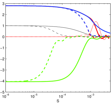
Figure 1: Evolution of the vector perturbations with wavenumber $k=0.02\text{Mpc}^{-1}$ (solid lines) and $k=0.2\text{Mpc}^{-1}$ (dashed lines). Thick lines are the velocities of the baryons (top), photons (until decoupling same as the baryon velocity) and neutrinos (bottom). Thin lines are ${\bar{\sigma}}$ (with ${\bar{\sigma}}_{0}=1$) and the photon anisotropic stress. The baryon velocity evolves independently of wavenumber on large scales, but is damped on small scales.

At early times the baryons and photons are tightly coupled, the opacity $\tau_{c}^{-1}\equiv S\text{n}_{e}\sigma_{\text{T}}$ is large. This means $v_{\gamma}\approx v$, and we can do an expansion in $\tau_{c}$ that is valid for $\epsilon\equiv\max(k\tau_{c},{\cal H}\tau_{c})\ll 1$. To lowest order

$$\bar{v}^{\prime} = -\frac{R{\cal H}\bar{v}}{1+R}+{\cal O}(\tau_{c})$$ (20)

where $R\equiv 3\rho_{b}/4\rho_{\gamma}$. The solution is

$$\bar{v}\approx\frac{\bar{v}_{0}}{1+R}$$ (21)

where $\bar{v}_{0}$ is the initial value. Hence if $\bar{v}_{0}\neq 0$, by decoupling $\bar{v}$ has only decayed an order unity factor depending on the matter and radiation density at the time. On smaller scales where $k\tau_{c}={\cal O}(1)$ before decoupling the perturbations are damped by photon diffusion, giving a characteristic fall off in perturbation power on small scales.

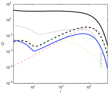
Figure 2: Typical CMB temperature (top solid), polarization EE (bottom solid), BB (dashed thick) and cross-correlation TE (dotted; absolute value) power spectra for regular vector modes assuming a primordial vector to scalar power ratio $\sim 10^{-3}$ and scale invariant vector mode spectrum $P_{\bar{\sigma}}$. The other dashed lines show the $B$-mode spectrum from weak lensing (peaking at $\ell\sim 1000$), and primordial tensors with initial power ratio $\sim 10^{-1}$ (peaking at $\ell\sim 100$).

We now perform a general series expansion in conformal time for the above equations in the early radiation dominated era to identify the regular primordial modes. We define $\omega\equiv\Omega_{m}{\cal H}_{0}/\sqrt{\Omega_{R}}$, where $\Omega_{R}=\Omega_{\gamma}+\Omega_{\nu}$, and ${\cal H}_{0}$ and $\Omega_{i}$ are the Hubble parameter and densities (in units of the critical density) today. The Friedmann equation gives

$$S=\frac{\Omega_{m}{\cal H}_{0}^{2}}{\omega^{2}}\left(\omega\eta+\frac{1}{4}\omega^{2}\eta^{2}+{\cal O}(\eta^{5})\right).$$ (22)

Defining the ratios $R_{\nu}\equiv\Omega_{\nu}/\Omega_{R}$, $R_{\gamma}\equiv\Omega_{\gamma}/\Omega_{R}$, $R_{b}\equiv\Omega_{b}/\Omega_{m}$, and keeping lowest order terms the regular solution (with zero initial anisotropies for $l>2$) is

$${\bar{\sigma}} = {\bar{\sigma}}_{0}\left(1-\frac{15}{2}\frac{\omega\eta}{4R_{\nu}+15}\right)$$ (23)

$$\bar{v}_{\gamma} = {\bar{\sigma}}_{0}\frac{4R_{\nu}+5}{R_{\gamma}}\left(\frac{1}{4}-\frac{3R_{b}}{16R_{\gamma}}\omega\eta\right)$$ (24)

$$\bar{v}_{\nu} = -\frac{{\bar{\sigma}}_{0}}{4}\frac{4R_{\nu}+5}{R_{\nu}}$$ (25)

$$I_{2} \equiv \frac{\Pi_{\nu}}{\rho_{\nu}}=-\frac{2}{3}\frac{k\eta}{R_{\nu}}{\bar{\sigma}}_{0}$$ (26)

where we have neglected small contributions from the scattering-suppressed photon anisotropic stress. This regular mode is the vector analogue of the neutrino velocity isocurvature mode discussed in Ref. Bucher et al. (2001). The shear ${\bar{\sigma}}$ is initially constant on super-horizon scales, supported by the growing anisotropic stress of the neutrinos. On sub-horizon scales in radiation domination it decays as the neutrino anisotropic stress starts to oscillate rather than grow.

The photon and neutrino vorticities are constant on super-horizon scales during radiation domination. This is consistent with angular momentum conservation because of the energy redshift. The photon vorticity is tightly coupled to the baryons, so both are initially nearly constant, with some decay due to drag from the baryons through matter radiation equality. On super-horizon scales there is only an order unity decay, so a significant large scale photon quadrupole will be present at low redshift to source a significant additional large scale polarization signal from reionization. The evolution is illustrated in Fig. 1.

On large scales the early ISW contribution is about 20% as ${\bar{\sigma}}$ decays as the matter becomes more dominant. On scales sub-horizon at recombination there is no ISW contribution as ${\bar{\sigma}}$ has already decayed. We neglect the effect of magnetic field generation by the photon-baryon vorticity Rebhan (1992).

.3 Observations

We now compute the observable CMB anisotropy signal. We define the dimensionless first order transverse vector $\sigma_{a}$ such that $\sigma_{ab}^{(1)}=D_{\langle a}\sigma_{b\rangle}$, and quantify the primordial vector modes by their power spectrum $P_{{\bar{\sigma}}}$ defined so that

$$\langle|{\bar{\sigma}}_{a}|^{2}\rangle=\int d\ln k\,\,P_{\bar{\sigma}}.$$ (27)

The corresponding expressions for the CMB temperature and polarization power spectra are derived in Lewis (2004).

To account for the small scale damping effect accurately, as well as a detailed treatment of recombination and reionization, we compute sample CMB power spectra numerically by a straightforward modification of CAMB. The CMB power spectra ($C_{l}$) depend on $P_{\bar{\sigma}}$. For a scale invariant spectrum, the temperature $C_{l}$ has a broad peak around $\ell\sim 50$, as shown in Fig. 2. The polarization power spectra peak at around $\ell\sim 500$, with the $B$-mode dominating in accordance with Ref. Hu and White (1997).

The large scale reionization signal is rather similar to that expected from tensor modes, and thus experiments aimed at detecting this tensor signal will also be sensitive to vector modes. Incomplete sky coverage only decreases the sensitivity by an order unity factor due to $E$-$B$ mode mixing Lewis et al. (2002); Lewis (2003) even on the largest scales. From Fig. 2 we see that the large scale $B$-modes are more sensitive to vector power by a factor of about 100, thus sensitive observations of tensor modes will also be good probes of regular vector modes. To distinguish the two one just needs to measure the spectrum at $\ell\gtrsim 100$ where the tensor power falls but the vector power continues to grow.

The dominant confusion on small scales is likely to be from weak lensing of the scalar modes, which peaks on similar scales. There are about $10^{6}$ observable modes, so one can ideally expect to detect a vector contribution $\sim 1/1000$ of the power of the lensing signal. Since they are of comparable power for a scale invariant primordial power spectrum ratio $P_{\chi}/P_{\bar{\sigma}}$ of $\sim 10^{-3}$ ($P_{\chi}$ is the power in the comoving curvature perturbation), this implies that vector modes with only $10^{-6}$ of the scalar power may be detectable irrespective of the tensor mode amplitude. Since the lensing signal is non-Gaussian, and in the absence of vector modes is partially subtractable Hirata and Seljak (2003); Kesden et al. (2003); Knox and Song (2002), the in-principle limit is probably much lower, though this depends on the spectrum of the vector modes. The ultimate limit may be around the level where there should be a sourced vector mode signal from second order effects Mollerach et al. (2004).

Primordial magnetic fields source a $B$-mode spectrum similar to that from primordial vector modes Subramanian et al. (2003). However the perturbations are expected to be highly non-Gaussian for magnetic fields and hence easily distinguishable from primordial vector modes if they are approximately Gaussian, at least until the lensing confusion limit. Magnetic fields also provide a constant source which partly compensate the damping, so there is more magnetic field vector mode power on very small scales. The detailed signature of magnetic fields in the CMB is discussed in Ref Lewis (2004), including the additional large scale signature from tensor modes.

Topological defects can also source similar $B$-mode spectra Seljak et al. (1997), though again the spectrum is expected to be non-Gaussian, and (at least for strings) there is more power on very small scales due to the continuous sourcing of the vector modes.

Conclusion

We have shown that regular primordial vector modes have a strong observational signature, allowing the possibility that tiny primordial amplitudes can be constrained from future high-sensitivity CMB polarization $B$-mode observations. Any signature of vector modes would be powerful evidence against simple inflationary models. The Planck satellite should be able to detect the $B$-mode signature from primordial vector modes at the $10^{-3}$ level, and distinguish them from tensor modes by the presence of small scale power. A full Bayesian joint analysis of all the CMB power spectra should be straightforward using MCMC techniques, and may give better constraints that suggested here. Separating a vector mode signal at the $10^{-6}$ level from that generated by lensing of scalar modes would be a serious challenge for the future.

References

- Bucher et al. (2001) M. Bucher, K. Moodley, and N. Turok, Phys. Rev. D62, 083508 (2001), eprint astro-ph/9904231.
- Subramanian et al. (2003) K. Subramanian, T. R. Seshadri, and J. D. Barrow, Mon. Not. Roy. Astron. Soc. 344, L31 (2003), eprint astro-ph/0303014.
- Lewis (2004) A. Lewis (2004), eprint astro-ph/0406096.
- Rebhan (1992) A. Rebhan, Astrophys. J. 392, 385 (1992).
- Bucher et al. (2004) M. Bucher, J. Dunkley, P. G. Ferreira, K. Moodley, and C. Skordis (2004), eprint astro-ph/0401417.
- Rebhan and Schwarz (1994) A. K. Rebhan and D. J. Schwarz, Phys. Rev. D50, 2541 (1994), eprint gr-qc/9403032.
- Ellis et al. (1983) G. F. R. Ellis, D. R. Matravers, and R. Treciokas, Ann. Phys. (N.Y.) 150, 455 (1983).
- Gebbie and Ellis (2000) T. Gebbie and G. F. R. Ellis, Ann. Phys. (N.Y.) 282, 285 (2000), eprint astro-ph/9804316.
- Challinor and Lasenby (1999) A. Challinor and A. Lasenby, Astrophs. J. 513, 1 (1999), eprint astro-ph/9804301.
- Hu and White (1997) W. Hu and M. White, Phys. Rev. D56, 596 (1997), eprint astro-ph/9702170.
- Challinor (2000) A. Challinor, Phys. Rev. D62, 043004 (2000), eprint astro-ph/9911481.
- Seljak and Zaldarriaga (1996) U. Seljak and M. Zaldarriaga, Astrophys. J. 469, 437 (1996), eprint astro-ph/9603033.
- Lewis et al. (2000) A. Lewis, A. Challinor, and A. Lasenby, Astrophys. J. 538, 473 (2000), eprint astro-ph/9911177.
- Lewis et al. (2002) A. Lewis, A. Challinor, and N. Turok, Phys. Rev. D65, 023505 (2002), eprint astro-ph/0106536.
- Lewis (2003) A. Lewis, Phys. Rev. D68, 083509 (2003), eprint astro-ph/0305545.
- Hirata and Seljak (2003) C. M. Hirata and U. Seljak, Phys. Rev. D68, 083002 (2003), eprint astro-ph/0306354.
- Knox and Song (2002) L. Knox and Y.-S. Song, Phys. Rev. Lett. 89, 011303 (2002), eprint astro-ph/0202286.
- Kesden et al. (2003) M. Kesden, A. Cooray, and M. Kamionkowski, Phys. Rev. D67, 123507 (2003), eprint astro-ph/0302536.
- Mollerach et al. (2004) S. Mollerach, D. Harari, and S. Matarrese, Phys. Rev. D69, 063002 (2004), eprint astro-ph/0310711.
- Seljak et al. (1997) U. Seljak, U.-L. Pen, and N. Turok, Phys. Rev. Lett. 79, 1615 (1997), eprint astro-ph/9704231.