Synthetic infrared images and spectral energy distributions of a young low-mass stellar cluster

Abstract

We present three-dimensional Monte Carlo radiative transfer models of a very young ($<10^{5}$ years old) low mass ($50\,\mathrm{M_{\sun}}$) stellar cluster containing 23 stars and 27 brown dwarfs. The models use the density and the stellar mass distributions from the large-scale smoothed particle hydrodynamics (SPH) simulation of the formation of a low-mass stellar cluster by Bate, Bonnell and Bromm. Using adaptive mesh refinement, the SPH density is mapped to the radiative transfer grid without loss of resolution. The temperature of the ISM and the circumstellar dust is computed using Lucy’s Monte Carlo radiative equilibrium algorithm. Based on this temperature, we compute the spectral energy distributions of the whole cluster and the individual objects. We also compute simulated far-infrared Spitzer Space Telescope (SST) images (24, 70, and 160 $\mathrm{\mathrm{\mu m}}$ bands) and construct colour-colour diagrams (near-infrared HKL and SST mid-infrared bands). The presence of accretion discs around the light sources influences the morphology of the dust temperature structure on a large scale (up to a several $10^{4}$ au). A considerable fraction of the interstellar dust is underheated compared to a model without the accretion discs because the radiation from the light sources is blocked/shadowed by the discs. The spectral energy distribution (SED) of the model cluster with accretion discs shows excess emission at $\lambda=$ 3–30 $\mathrm{\mu m}$ and $\lambda>500\,\mathrm{\mu m}$, compared to that without accretion discs. While the former is caused by the warm dust present in the discs, the latter is cause by the presence of the underheated (shadowed) dust. Our model with accretion discs around each object shows a similar distribution of spectral index (2.2–20 $\mathrm{\mathrm{\mu m}}$) values (i.e. Class 0–III sources) as seen in the $\rho$ Ophiuchus cloud. We confirm that the best diagnostics for identifying objects with accretion discs are mid-infrared ($\lambda=$ 3–10 $\mathrm{\mu m}$) colours (e.g. SST IRAC bands) rather than HKL colours.

1 Introduction

Systematic investigations of young stellar objects (YSOs) in a star-forming cloud including comparative studies of theoretical predictions and observations are important for understanding the stellar/substellar formation processes. Examples of well-studied star-forming clouds are the Orion Trapezium Cluster, NGC 2024, and the $\rho$ Ophiuchus and Taurus-Auriga clouds. Recent observations of young clusters have been used to determine circumstellar disc frequencies, disc mass distributions, initial mass functions (IMFs) and evolutional stages of the objects in the clusters. It has been shown that JHKL and HKL colour-colour diagrams are particularly effective in identifying the presence of circumstellar discs (e.g. Kenyon & Hartmann 1995; McCaughrean et al. 1995; Lada et al. 2000; Haisch et al. 2001). The spectral indices (Lada, 1987) or the slopes of observed spectral energy distributions (SEDs) of YSOs from near- to mid-infrared wavelengths are used to classify SEDs, and the classification scheme is often related to the evolutionary stages of YSOs (e.g. Adams, Lada, & Shu 1987; Myers et al. 1987). The distribution of circumstellar disk masses in young clusters can be measured from millimetre continuum emission (e.g. Eisner & Carpenter 2003 for NGC 2024). Determining IMFs of young clusters requires evolutionary models (e.g. D’Antona & Mazzitelli 1997; Baraffe et al. 1998) and infrared spectroscopy for spectral type identifications (e.g. Luhman & Rieke 1999 for the $\rho$ Ophiuchus cloud).

Bate, Bonnell, & Bromm (2003) presented results from a very large three-dimensional (3-D) smoothed particle hydrodynamics (SPH) simulation of the collapse and fragmentation of a 50 $\mathrm{M_{\sun}}$ turbulent molecular cloud to form a stellar cluster. The calculation resolved circumstellar discs down to $\sim 10$ au in radius and binary stars as close as 1 au. Although some observational predictions, such as the IMF and binary fraction, may be gleaned directly from a hydrodynamical simulation of stellar cluster formation, the principal observable characteristics (optical, near-IR, IR, and sub-millimetre images and spectra) require further detailed radiative transfer modelling. The density distribution of such hydrodynamical calculations is very complicated, and the corresponding radiative transfer must be also performed in full 3-D.

There are two basic approaches to 3-D radiative transfer problems:  grid based methods (e.g. finite differencing, short- and long- characteristic methods), and particle (photon) based methods, i.e. Monte Carlo. Examples of the first kind are Stenholm, Störzer, & Wehrse (1991), Folini et al. (2003) and Steinacker, Bacmann, & Henning (2002). Those of the second kind include Witt & Gordon (1996), Pagani (1998), Wolf, Henning, & Stecklum (1999), Harries (2000) and Kurosawa & Hillier (2001). The advantages of the second approach are, for example, the flexibility to treat a complex density distribution and a complex scattering function. Readers are referred to Steinacker et al. (2003) and Pascucci et al. (2004) for more extensive discussion on the advantages and disadvantages of these two different methods.

The temperature of the interstellar and circumstellar dust in the cluster must be calculated in order to determine the source function of the dust emission. The radiative equilibrium temperature of the dust particles can be found using the Monte Carlo method (e.g. Lefevre, Bergeat, & Daniel 1982; Wolf et al. 1999; Lucy 1999; and Bjorkman & Wood 2001). The technique used by Lucy (1999) takes into account the fractional photon absorptions between two events of a ‘photon packet’; hence, it works well even in the limit of low opacity. Bjorkman & Wood (2001) used the immediate re-emission technique, in which radiative equilibrium is forced at each interaction with the dust. A photon is re-emitted immediately after an absorption event using a product of the dust opacity and the difference between the Planck function with a current temperature and that with a new temperature corresponding to the radiative equilibrium of the dust that absorbed the photon. Unlike the method of Lucy (1999), this does not require a temperature iteration if the opacity is independent of temperature. Alternatively, Niccolini, Woitke, & Lopez (2003) used the ray-splitting method showing its effectiveness for both low and high optical depth media.

Here we aim to simultaneously resolve the dust on parsec and sub-stellar-radius spatial scales, whilst including multiple radiation sources. To overcome the resolution problem, we have implemented an adaptive mesh refinement (AMR) scheme in the grid production process of the TORUS radiative transfer (Harries, 2000). See also Wolf et al. (1999), Kurosawa & Hillier (2001) and Steinacker et al. (2002) for a similar gridding scheme in a radiative transfer problem. The method described by Lucy (1999) is used to compute dust temperatures in our models.

The objectives of this paper are: 1. to compute observable quantities by solving the radiative transfer problem using a complex density distribution from the SPH calculation by Bate et al. (2003); 2. to analyse the predicted observational properties of the cluster generated in the simulation of Bate et al. (2003) at a distance of 140 pc which corresponds to the distance of nearby star-forming regions such as Taurus-Auriga and the $\rho\,$Ophiuchus cloud (e.g. Bertout, Robichon, & Arenou 1999).

In Section 2, we describe the details of our models. The results of the model calculations are given in Section 3. The conclusions are summarised in Section 4.

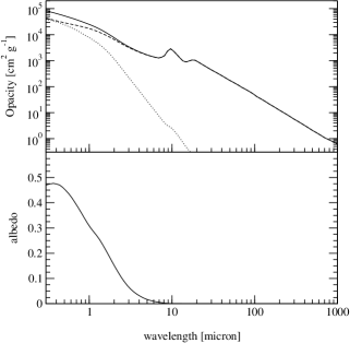
Figure 1: Top: The scattering (dotted line), the absorption (dashed line), and the total (solid line) opacities of the grain model, described in Section 2.5, are shown as functions of wavelength. Bottom: The corresponding albedo of the grains is shown as a function of wavelength.

2 Methods

We calculate the main observable quantities of the low mass (50 $\mathrm{M_{\sun}}$) cluster formation simulation by Bate et al. (2003). There are four basic steps in this process:

1. Create the AMR grid from the SPH particle positions and the density at each particle. The density is assigned to the grid cells during the grid construction.

2. Calculate the luminosity and the effective temperature of each light source (in the SPH calculation) based on its mass using an evolutional model of young stars (D’Antona & Mazzitelli 1998; Censori & D’Antona 1998).

3. Compute the temperature of the dust in the cluster using the Monte Carlo radiative equilibrium model of Lucy (1999).

4. Compute the SEDs and the images using the Monte Carlo radiative transfer code, TORUS.

2.1 The SPH model

Bate et al. (2002a, 2002b, 2003) presented a numerical SPH simulation of star cluster formation resolving the fragmentation process down to the opacity limit ($\sim$0.005 M_⊙). The initial conditions consist of a large-scale, turbulent molecular cloud with a mass of 50 $\mathrm{M_{\sun}}$ and a diameter of 0.375 pc (77 400 au). The initial temperature of the cloud was 10 K, and its corresponding mean thermal Jeans mass was 1 $\mathrm{M_{\sun}}$ (i.e. the cloud contained 50 thermal Jeans masses). The free-fall time of the cloud was $t_{\mathrm{ff}}=6.0\times 10^{12}\,\mathrm{{s}}=1.90\times 10^{5}\,\mathrm{{yr}}$. Similar to the method used by Ostriker, Stone, & Gammie (2001), they imposed an initial supersonic turbulent velocity field on the cloud by generating a divergence-free random Gaussian velocity field with a power spectrum $P\left(k\right)=k^{-4}$ where $k$ is the wave number. This was chosen to reproduce the observed Larson scaling relations (Larson, 1981) for molecular clouds. The total number of particles used in the simulations was $3.5\times 10^{6}$, making it one of the largest SPH calculations ever performed. Approximately 95 000 CPU hours on the SGI Origin 3800 of the United Kingdom Astrophysical Fluids Facility (UKAFF) were spent on the calculation.

We use the output from the final time step of the SPH calculation as the input for the radiative transfer code. The time of the data dump is 0.27 Myr, at which the cluster contains 50 point masses (stars and brown dwarfs). Each SPH data point contains the position ($x$, $y$, $z$), the velocity components ($V_{x}$, $V_{y}$, $V_{z}$) and the density ($\rho$). The velocity information is not used in our calculation since we are only interested in continuum emission, but these data may be used in future calculations of molecular line emission. The total masses contained in the stars and the molecular gas are $6\,\mathrm{M_{\sun}}$ and $44\,\mathrm{M_{\sun}}$ respectively.

2.2 Source catalogue

The SPH data provides the masses of the stellar objects (23 stars and 27 brown dwarfs), ranging from 0.005 to 0.731 $\mathrm{M_{\sun}}$ (see Table 1). Since the Monte Carlo radiative transfer code requires the luminosity ($L$), the effective temperature ($T_{\mathrm{{eff}}}$) and the radius ($R_{*}$) of each star, we computed them indirectly from evolutionary models. For a given age and mass of each star and brown dwarf, the luminosity and the temperature are interpolated from the 1998 updated version of data by D’Antona & Mazzitelli (1998) and Censori & D’Antona (1998) available on their website (http://www.mporzio.astro.it/~dantona/prems.html). Although the actual age of the stars and brown dwarfs in the SPH data of Bate et al. (2003) ranges from $\sim$2 000 to $\sim$70 000 years old, we make the pragmatic assumption that all the objects are 0.25 Myr old because we believe that at young ages the stellar radii are overestimated (c.f., Baraffe et al. 2002), leading to unrealistically high luminosities. Adopting models with ages of 0.25 Myr provides more plausible radii (and therefore luminosities), while the change in temperature over this timespan is modest (Baraffe et al. 2002).

The radii are estimated from $L=4\pi R^{2}\sigma T_{\mathrm{{eff}}}^{4}$ where $\sigma$ is the Stefan-Boltzmann constant. The results are summarised in Table 1. The combined luminosity of all 50 sources is $16.8\,\mathrm{L_{\sun}}$.

We take the spectral energy distribution of the individual stars to be blackbodies. Although we recognise that the spectra of the objects (particularly at the lowest masses) may be significantly structured due to molecular opacity, the vast majority of the stellar flux is reprocessed by the circumstellar dust and the precise form of the input spectrum is unimportant.

Landscape table to go here. (Table 1 attached to the end of paper.)

Table 1:

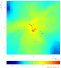
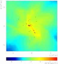
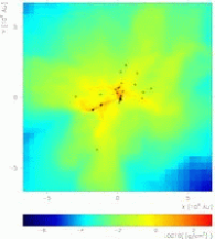
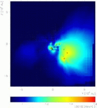
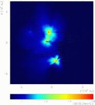
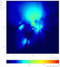
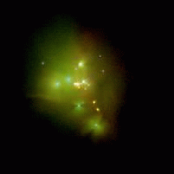
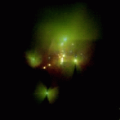
Figure 2: Top: the log of dust column density (in $\mathrm{g~{}cm^{-2}}$) along $x$, $y$ and $z$ axes from left to right respectively (both Models I and II). Middle: The temperature on $x=0$, $y=0$, and $z=0$ planes from left to right (Model II). Bottom: The composite images of SST MIPS bands – 24 $\mathrm{\mu m}$ (blue) 70 $\mathrm{\mu m}$ (green) and 160 $\mathrm{\mu m}$ (red) – along the x, y and z axes from left to right respectively (Model II). The black circles in the column density and temperature plots indicate the locations of the stars and brown dwarfs projected on each plane.

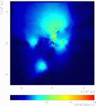
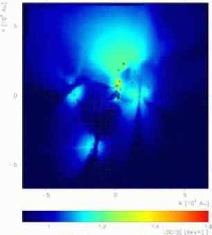
Figure 3: Log-scale temperature maps (in kelvins) from Model I (left) and Model II (right) on the $z=0$ plane. The circles indicate the positions of stars and brown dwarfs projected on the plane. The temperature of the dust shadowed by the accretion discs (left) is significantly lower than that of Model I. Although the same colour scale is used for both maps, the actual maximum dust temperatures for Model I and Model II are around 300 K and 1600 K respectively.

2.3 The grid construction (AMR)

The algorithm used to construct the grid in this paper is very similar to that used in Kurosawa & Hillier (2001). More detailed discussion of the AMR grid construction and the data structure used in our model are given in Symington (2004). Starting from a large cubic cell (with size $d$) which contains all the SPH particles, we first compute the density of the cell by averaging the density values assigned to the particles. Then, the density is multiplied by the volume of the cell ($d^{3}$) to find the total mass ($M$) in the cell. If the mass is larger than a threshold mass ($M_{\mathrm{th}}$), which is a user defined parameter, this cell is split into 8 subcells with size $d/2$. If the mass of the cell is less than the threshold, it will not be subdivided. Recursively, the same procedure is applied to all the subcells until all the cells contain a mass less than the threshold ($M<M_{\mathrm{th}}$). Our largest models split the grid on 27 levels, i.e. they incorporate a dynamical range of $2^{27}\approx 10^{8}$. The average optical depth across a cell is about $1.5$ at $2\,\mu\mathrm{m}$ which corresponds to the peak of a blackbody radiation curve ($B_{\nu}$) with the mean temperature ($T=2900\,\mathrm{K}$) of the stars and brown dwarfs in our models.

2.4 Temperature calculation

The dust temperature is computed using the method described by Lucy (1999). The material is assumed to be in local thermodynamic equilibrium (LTE) and in radiative equilibrium. The former indicates that the source function ($S_{\lambda}$) is described solely by the Planck function, $B_{\lambda}$, for all wavelengths $\lambda$:

$$S_{\lambda}=B_{\lambda}\left(T\right)$$ (1)

where $T$ is the temperature of the dust. The latter indicates that the total energy absorbed by a volume element per unit time is exactly same as the total amount of energy emitted by the volume in unit time:

$$\int_{0}^{\infty}\kappa_{\lambda}B_{\lambda}d\lambda=\int_{0}^{\infty}\kappa_{\lambda}J_{\lambda}d\lambda\,$$ (2)

where $\kappa_{\lambda}$ and $J_{\lambda}$ are the thermal absorption coefficient and the specific mean intensity respectively. The expression can be derived by integrating the radiative transfer equation, $dI_{\lambda}/dl=\rho\kappa_{\lambda}\left(S_{\lambda}-I_{\lambda}\right)$, over all wavelengths and solid angles ($\Omega$), using the LTE condition (equation 1) and flux conservation (c.f., Chandrasekhar 1960). By rewriting equation 2 using the Planck mean ($\bar{\kappa}_{\mathrm{p}}$) and the absorption mean ($\bar{\kappa}_{J}$), it becomes:

$$J=\frac{\bar{\kappa}_{\mathrm{p}}}{\bar{\kappa}_{J}}\,B\left(T\right)$$ (3)

where $\bar{\kappa}_{\mathrm{p}}$ and $\bar{\kappa}_{J}$ are defined as:

$$\bar{\kappa}_{\mathrm{p}} \equiv \frac{\int_{0}^{\infty}\kappa_{\lambda}B\left(T\right)_{\lambda}d\lambda}{\int_{0}^{\infty}B_{\lambda}\left(T\right)d\lambda}=\frac{\pi\int_{0}^{\infty}\kappa_{\lambda}B_{\lambda}\left(T\right)d\lambda}{\sigma T^{4}}$$ (4)

$$\bar{\kappa}_{J} \equiv \frac{\int_{0}^{\infty}\kappa_{\lambda}J_{\lambda}d\lambda}{\int_{0}^{\infty}J_{\lambda}d\lambda}=\frac{\int_{0}^{\infty}\kappa_{\lambda}J_{\lambda}d\lambda}{J}\,,$$ (5)

and the (wavelength integrated) mean intensity $J$ is

$$J=\int_{0}^{\infty}J_{\lambda}d\lambda\,.$$ (6)

Using the $\Lambda$ operator (e.g. Mihalas 1978), the formal solution of the radiative transfer equation can be written as:

$$J=\Lambda\left[S\right]=\Lambda\left[B\left(T\right)\right]\,.$$ (7)

This problem is often solved by iteration starting from some initial temperature structure. As noted by Lucy (1999), equation 3 is indeed in the form of the formal solution; hence, we can use an iterative scheme to obtain the temperature. Note that using $B\left(T\right)=\sigma T^{4}/\pi$ in equation 3, we have:

$$T=\left(\frac{\pi\bar{\kappa}_{J}}{\sigma\bar{\kappa}_{\mathrm{p}}}\,J\right)^{1/4}\,.$$ (8)

In addition, Lucy (1999) explicitly used flux conservation as a constraint when computing $\bar{\kappa}_{J}J$ and $\bar{\kappa}_{\mathrm{p}}$ in each iteration step.

Our basic iteration scheme is summarised as follows:

1. Using the current temperature ($T_{i}$) from the $i$-th iteration step, estimate the values of $\bar{\kappa}_{J}J$ and $\bar{\kappa}_{\mathrm{p}}$ for each cell using the Monte Carlo method (Lucy, 1999).

2. Evaluate the new temperature ($T_{i+1}$) using equation 8.

3. Check for convergence. If the model has not converged, go back to (i).

The model is considered to have converged when

$$\delta=\frac{\Delta\bar{T}_{i+1}-\Delta\bar{T}_{i}}{\frac{1}{2}\left(\Delta\bar{T}_{i+1}+\Delta\bar{T}_{i}\right)}<0.05$$ (9)

where $\Delta\bar{T}_{i}=\bar{T}_{i}-\bar{T}_{i-1}$, and $\bar{T}_{i}$ is the mean temperature of all cells in the $i$-th iteration.

Harries et al. (2004) presented test calculations for the dust temperature using our Monte Carlo model for a spherical shell (1-D) and a disc (2-D), and showed the results agree with those of well-established existing codes (e.g. Ivezić et al. 1999; Pascucci et al. 2004).

2.5 Dust model

To calculate the dust scattering and absorption cross-sections as functions of wavelength, we have used the optical constants of Draine & Lee (1984) for amorphous carbon grains and Hanner (1988) for silicate grains. For simplicity, the model uses the standard interstellar medium (ISM) power-law size distribution function (e.g, Mathis, Rumpl, & Nordsieck 1977):

$$n\left(a\right)\propto a^{-q}$$ (10)

for $a_{\mathrm{\mathrm{min}}}<a<a_{\mathrm{max}}$ with $q=3.5$, $a_{\mathrm{\mathrm{min}}}=5\times 10^{-3}\,\mathrm{\mathrm{\mu m}}$ and $a_{\mathrm{\mathrm{min}}}=0.25\,\mathrm{\mathrm{\mathrm{\mu m}}}$. The relative number of each grain is assumed to be that of solar abundance, C/H$\sim 3.5\times 10^{-4}$ (Anders & Grevesse, 1989) and Si/H$\sim 3.6\times 10^{-5}$ (Grevesse & Noels, 1993) which are similar to values found in the ISM model of Mathis et al. (1977) and Kim, Martin, & Hendry (1994). Similar abundances were used in the circumstellar disc models of Cotera et al. (2001) and Wood et al. (2002b). Figure 1 shows the resulting opacities and albedo as functions of wavelength.

Assuming spherical dust particles, the Mie-scattering phase matrix is pre-tabulated and used in our calculations, instead of using an approximate scattering phase function (e.g. Henyey & Greenstein 1941). We assume the same dust size distribution in the ISM and the circumstellar discs, i.e. the circumstellar discs do not contain larger grains. If larger grain sizes are chosen for the circumstellar dust, the wavelength dependency of the dust opacity (Figure 1) will be shallower than that of the ISM dust (Wood et al., 2002b). As a result, this may change the slope of model SEDs in sub-millimetre wavelength range (c.f. Beckwith et al. 1990; Beckwith & Sargent 1991).

2.6 Images and SED calculation

Once the temperature structure has converged, the source function is known everywhere in the model space (assuming LTE). Using this information, we simulate the observable quantities, namely the SEDs and the images. The Monte Carlo radiative transfer method is used again to propagate the photons, and project them on to an observer’s plane on the sky. The basic method used here is presented in e.g. Hillier (1991) and Harries (2000).

The following sets of filters are used in our calculations: standard J, H, K and L; SST Infrared Array Camera (IRAC) at 3.6, 4.5, 5.8 and 8.0 $\mathrm{\mu m}$; the SST Multiband Imaging Photometer (MIPS) at 24, 70, and 160 $\mathrm{\mu m}$.

2.7 Accretion disc model

The SPH simulations of Bate et al. (2003) do not resolve scale sizes less than $\sim 10$ au; hence, accretion discs very close to stars and brown dwarfs are not included. These missing accretion discs are potentially very important in the calculations of the SED and the images. Although large accretion discs exist around some objects in the SPH calculation, they do so only at distances $>10\,\mathrm{au}$ from the central object. To investigate the effect of the warm dust very close to the objects, we insert discs using the density described by the steady $\alpha$-disc ‘standard model’ (Shakura & Sunyaev 1973; Frank, King, & Raine 2002).

$$\rho_{\mathrm{d}}\left(r,z\right)=\Sigma\left(r\right)\,\frac{1}{\sqrt{2\pi}h\left(r\right)}e^{-\left(\frac{z}{2h\left(r\right)}\right)^{2}}$$ (11)

where $r$ is the cylindrical radius expressed in units of the disc radius $R_{\rm d}$, and $h$ and $z$ are the scale height and the distance from the disc plane, respectively. $\Sigma$ is the surface density at the mid-plane. The mid-plane surface density and the scale height are given as:

$$\Sigma\left(r\right)=\frac{5M_{\mathrm{d}}}{8\pi R_{\mathrm{d}}^{2}}\,r^{-3/4}$$ (12)

where $M_{\mathrm{d}}$ is the disc mass.

$$h\left(r\right)=0.05\,R_{\mathrm{d}}\,r^{9/8}\,.$$ (13)

Note that the mid-plane surface density, predicted by the irradiated disk model of D’Alessio et al. (1998), has a slightly steeper radial dependency ($\Sigma\propto r^{-1}$).

The inner radius of the disc is set to $R_{\mathrm{i}}=6\,R_{*}$ which is the assumed dust destruction radius of our model (c.f., Wood et al. 2002b). The disc mass, $M_{\mathrm{d}}$, is assumed to be 1/100 of the central object’s mass, and the disc radius ($R_{\mathrm{d}}$) to be 10 au unless it has a binary companion. When an object is in a binary system, the disc radius is assigned to be 1/3 of the binary separation (e.g. Artymowicz & Lubow, 1994). Finally, the orientations of the discs are assigned from the spin angular momentum of the objects in the SPH simulation which keeps track of the angular momentum of the gas accreted by the objects.

3 Results

We present results from two different models: I. the density structure is exactly the same as in the SPH simulation (i.e. there is no circumstellar material within 10 au of any star) and II. the density structure is from the SPH simulation with the addition of accretion discs as described in Section 2.7. The total number of cells used in Models I and II are 2,539,440 and 25,223,192 respectively. The corresponding cell subdivision levels are 16 and 27 for Models I and II, providing smallest cell sizes of 1 au and $\sim 0.1\,\mathrm{R_{\sun}}$ respectively. Table 2 summarises the basic model parameters.

Table 2: Basic Model Parameters

	Model I	Model II
Size of the largest cell	$2\times 10^{18}\,\mathrm{cm}$	$2\times 10^{18}\,\mathrm{cm}$
Size of the smallest cell	1 au	$\sim 0.1\,\mathrm{R_{\sun}}$
Discs within 10 au?	No	Yes
Number of grid cells	2,539,440	25,223,192
AMR subdivision levels	16	27

3.1 Density and temperature maps

We assume a gas-to-dust mass ratio of 100 (c.f., Liseau et al. 1995), and assign the dust density of each cell accordingly. The resulting dust column-density maps along $x$, $y$ and $z$ axes for Model II are given in the top row of Figure 2. On this scale, the column density maps for Model I look exactly the same except that the value of the maximum column density is lower.

The results from the radiative equilibrium temperature calculations for Models I and II are shown in Figure 3. Approximately 500 CPU hours were spent on the SGI Origin 3800 of the UKAFF for computing temperatures for Model I, and 2400 CPU hours for Model II. Although the same colour scale is used for both models in Figure 3, the maximum dust temperatures found in the whole domain of the models are about 300 K and 1600 K for Models I and II, respectively. In both models, the average temperature of the ISM dust is around 20 K. The temperature maps for Model II on $x=$0, $y=0$, and $z=0$ planes are also given in the middle row of Figure 2. The angle averaged optical (at $\lambda=5500$ Å) using 600 random directions from the centre of the cluster to the outer boundary of the models is 93 ($A_{V}=102$).

It is clear from the temperature maps of Model II that the presence of the circumstellar discs influences the morphology of the temperature structure. Discs affect the temperature of the dust even on a large scale (up to a several $10^{4}$ au). In Model II, the dust shadowed by the accretion disc has a lower temperature than that of Model I. The radiation field near the stars becomes anisotropic/bipolar when circumstellar discs are present.

The density and the temperature maps around our typical star, object 4 (see Table 1), are shown in Figure 4 (upper right and left) for Model II. On the same scale, no structure will be seen in a similar plot for Model I as explained in Section 2.5. The density map clearly shows that the cell size increases as the distance from the star (located at the centre) increases, and also as the distance from the mid-plane of the disc increases. In the temperature map, the hole around the star is created because the temperature of the low density material present in the background reaches 1600 K, the dust sublimination temperature; therefore, those cells are removed from the computational domain. We note that temperatures of the inner-most part of discs also can become greater than 1600 K, and the grid cells in this part of the discs will be removed. As a consequence, the inner radius may be slightly larger than an initial value ($R_{\mathrm{i}}=6\,R_{*}$).

In the lower left of Figure 4, the density at the mid-plane of the disc is plotted as a function of the distance from the star. The slope of the density plot is $\sim-15/8$ as it should be according to equations 11–13. Similarly, the temperature at the mid-plane is plotted as a function of the distance from the star in the lower right of the same figure. The slope at the outer part of the disc (0.3–10 au) is $-0.45$ which is consistent with that of Whitney et al. (2003b). This is slightly smaller than the value for an optically thin disc ($-0.4$), with an absorption coefficient inversely proportional to wavelength, heated by stellar radiation (c.f., Spitzer 1978; Kenyon et al. 1993; Chiang & Goldreich 1997). In the inner part of the disc (0.1–0.12 au), the slope quickly increases. A similarly rapid rise of the slope is seen in the no-accretion-luminosity disc model of Whitney et al. (2003b) as shown in their Fig. 6.

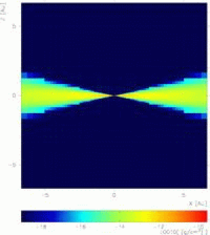
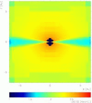
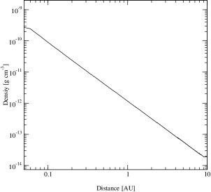
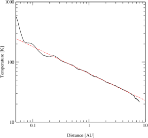
Figure 4: The density (upper left) and the temperature (upper right) maps around a typical star (object 4 in Table 1), are shown for Model II. No material would be seen in a similar plot for Model I on the same scale due to the absence of small scale discs. In the temperature map, the hole around the star was created because the temperature of the low density material present in the background became more than 1600 K, the dust sublimination temperature, and the cells were removed from the computational domain. The density at the mid-plane of the disc is plotted as a function of the distance from the star (lower left). The temperature at the mid-plane is plotted as a function of the distance from the star (lower right). The temperature slope of the outer part of the disc (0.3–10 au) is $-0.45$ (dash-dot line) which is consistent with that of Whitney et al. (2003b). This is slightly smaller than the value for an optically thin disc ($-0.4$), with an absorption coefficient inversely proportional to wavelength, heated by stellar radiation (Spitzer 1978; Kenyon et al. 1993; Chiang & Goldreich 1997). In the inner part of the disc (0.1–0.12 au), the slope quickly increases. A similar rapid raise of the slope is also seen in Fig. 6 of Whitney et al. (2003b).

3.2 Spectral energy distributions of the cluster

The SEDs from Models I and II are shown in Figure 5 along with the SED of the combined naked stars (the stars without the ISM and the circumstellar dust) and a 20K blackbody radiation spectrum. The observer is placed at a distance of 140 pc (on the $+z$ axis) from the cluster. Both models show peaks around $2\,\mathrm{\mu m}$ and $200\,\mathrm{\mu m}$. The first peak corresponds to that of stellar emission, and the latter corresponds to the emission from the relatively low temperature ISM dust. In Model I, the $200\,\mathrm{\mu m}$ peak is prominent, indicating that the most of the ISM dust has $T\approx 20\,\mathrm{K}$.

The most noticeable differences between the two models are the flux levels at $\lambda=$ 3–30 $\mathrm{\mu m}$ and $\lambda>500\,\mathrm{\mu m}$. The excess emission of Model II at $\lambda=$ 3–30 $\mathrm{\mu m}$ is due to the warm dust present in the accretion discs. This emission arises from the reprocessing of photospheric emission by the inner discs into the observer’s line-of-sight, and is dominated by a handful of objects (in particular object numbers 7 and 8, which constitute an ejected binary system). The excess emission in the far infrared ($\lambda>500\,\mathrm{\mu m}$) in Model II is caused by the presence of a larger amount of cold ($T<20\,\mathrm{K}$) dust. As we can see from Figure 3, a considerable fraction of the ISM in Model II is underheated compared to the dust in Model I because the radiation from the light sources is blocked/shadowed by the accretion discs. The SED of Model II is very similar to the observed SED of a young star forming region (ISOSS J 20298+3559-FIR1) with mass around 120$\mathrm{M_{\sun}}$ presented by Krause et al. (2003). They showed that a Planck function with the temperature corresponding to the peak of the SED ($T=19\,\mathrm{K}$) underestimates the flux levels observed at $\lambda<60\,\mathrm{\mu m}$ and $\lambda>500\,\mathrm{\mu m}$.

We note that the slope of the SEDs at sub-milimetere wavelengths is sensitive to the wavelength dependency of the dust absorption coefficient ($\kappa$). If a shallower wavelength dependency of the dust opacity is introduced for the discs in Model II, the slope of the SEDs in the sub-millimetre wavelength range may change (e.g. Beckwith et al. 1990; Beckwith & Sargent 1991).

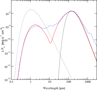
Figure 5: The spectral energy distributions (SEDs) from Model I (solid line) & Model II (dash-dot line) compared with the 20 K blackbody radiation curve (dashed line) and the SED of naked (without the ISM and circumstellar dust) stars and brown dwarfs (dotted line). Both models show peaks around 2 $\mathrm{\mu m}$ and 200 $\mathrm{\mu m}$. The first peak corresponds to that of stellar emission, and the latter corresponds to emission from the ISM dust with $T\sim 20~{}\mathrm{K}$. The excess emission between 3 $\mathrm{\mu m}$ and 30 $\mathrm{\mu m}$ for Model II is caused by the warm dust in the accretion discs. The excess emission in the far infrared ($\lambda>500~{}\mathrm{\mu m}$) seen in Model II is due to the emission from the increased amount of cold ($T<20~{}\mathrm{K}$) dust due to disc shadowing.

3.3 Spectral energy distributions of stars and brown dwarfs

Detailed studies of isolated objects have been performed by Wood et al. (2002a) and Whitney et al. (2003a), covering the evolution of the SED from the protostar through to the remnant disc stage. These models are an excellent point of comparison for our model SEDs, which are based on the density structures predicted for a ’realistic’ star-forming cloud. The circumstellar material from the SPH calculation is however significantly more complex than the axisymmetric, idealized models cited above.

To calculate the SEDs of individual objects, we have used the same density and temperature structures as in Section 3.1 with some restrictions. Firstly, a cylinder of radius 50 au with its centre passing through an observer (situated on the $z$-axis) and the centre of an object is considered. (The diameter of this cylinder roughly corresponds to a 0.7 arcsec aperture at 140 pc). We note that Whitney et al. (2003a) used 1000 au and 5000 au aperture sizes to compute colours of protostars, and found that the colours can change depending on the aperture size adopted. In our calculations, we use a smaller (50 au) aperture because the stellar densities in the cluster are such that larger apertures may include significant contributions from neighbouring objects. Secondly, the dust emission, absorption and scattering outside of the cylinder are turned off. Thirdly, only the star under consideration can emit the photons. With these restrictions, we have performed the Monte Carlo radiative transfer calculations for each object in Table 1. The results are shown in Figure 6. Because of the restrictions used, some scattered flux contribution from the outside of the cylinder might be missing in the resulting SEDs, and the contamination due to the dust emission from the disc of a companion might be present in the SEDs if a star is in a binary system. Note that the binary pairs in the source catalogue (Table 1) are 3–10, 7–8, 20–22, 44–42, 26–40, 39–41 and 45–38. Readers are referred to table 2 of Bate et al. (2003) for binary parameters (separations, eccentricities and so on). As we can see from the panels of Figure 6, the sources are deeply embedded in the cloud, and about half of them show little flux in the optical. The SEDs are very similar to those of the Class 0 model in Whitney et al. (2003a). The silicate absorption feature at 10 $\mathrm{\mu m}$ becomes more prominent for objects with higher extinction.

We have computed $K$ band magnitude, the flux at 8 $\mathrm{\mu m}$ ($F_{8}$) and 24 $\mu m$ ($F_{24}$) based on the SEDs, and extinction ($A_{V}$) by integrating the opacities between each object and an observer. The results are placed in Table 1. For Model II, the inclinations of the discs with respect to an observer on $+z$ axis (that used in the calculation of the global SEDs) are also listed in the same table. The number of objects brighter than $K=20$ are 26 and 30 objects for Model I and Model II respectively.

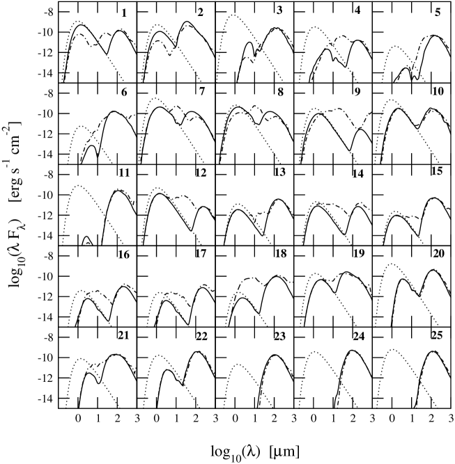
Figure 6: Atlas of individual spectral energy distributions (SEDs). The SEDs from Model I are shown in solid lines and those from Model II in dash-dot lines. The input source SEDs are presented in dotted lines. The numbers shown in upper right hand corner of each plot correspond to the object ID number in Table 1. To compute the SED from each star, the same density and temperature structures in section 3.1 are used with some restrictions (see text for detail). As we can see from the SEDs, the sources are deeply embedded in a cloud, and about the half of them show little flux in the optical. The silicate absorption feature at 10 $\mathrm{\mu m}$ becomes more prominent for objects with higher extinction.

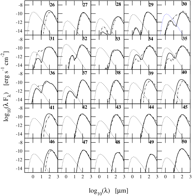
Figure 6: Concluded.

Using the flux between 2.2–10.2 $\mu$m, the SEDs in Figure 6 are classified based on the spectral index $\left(a\right)$ as defined by Wilking, Lada, & Young (1989):

$$a=\frac{d\log\left(\lambda F_{\lambda}\right)}{d\log\lambda}.$$

We have used the monochromatic fluxes at K (2.2 $\mathrm{\mu m}$), L (3.6 $\mathrm{\mu m}$), M (4.8 $\mathrm{\mu m}$), N (10.2 $\mathrm{\mu m}$) to compute the values of $a$ via least-squares fits (e.g. Greene et al. 1994; Haisch et al. 2001). The classification scheme of Greene et al. (1994) is adopted in our analysis. The sources with $a>0.3$ are classified as ‘Class I’, $-0.3<a\leq 0.3$ as ‘flat spectrum’, $-1.6<a\leq-0.3$ as ‘Class II’, and $a<-1.6$ as ‘Class III’ YSOs. In addition to this scheme, we classify sources to be Class 0 (Andre et al. 1993) if the ratio of $\log\lambda F_{\lambda}$ values at $\lambda=160\,\mathrm{\mu m}$ (SST MIPS) and at $\lambda=2.2\,\mathrm{\mu m}$ ($K$ band) is greater than 3.0 (c.f., Fig. 3 of Whitney et al. 2003a). The results are placed in Table 1 for both models. Out of 50 objects, there are 27 Class 0, no Class I, no flat spectrum, 11 Class II and 12 Class III objects for Model I, and there are 28 Class 0, 9 Class I, 4 flat spectrum, 6 Class II, and 3 Class III objects for Model II. Note that even though all objects are $<0.07$ Myrs old, there is a mixture of Class 0–III objects. Thus, the class of an object does not necessarily relate to its evolutionary stage. Whitney et al. (2003a) also pointed out the degeneracy problem of the SEDs from Class I and Class II objects, and that their colours look very similar to each other for some combinations of disc inclinations and luminosities.

Figure 7 shows the distribution of the spectral index values. The upper row in the figure shows the histograms of the index values from all 50 objects while the lower part shows those created from ’observable’ ($K<20$) objects. The histograms based on all objects peak around $a=0$ for Model I and II, and the distributions are skewed. On the other hand, the number of the objects with $K<20$ for Model II look more evenly distributed around $a=0$ (lower right in Figure 7). The latter is very similar to the spectral index distribution of the $\rho$ Ophiuchus cloud presented in Fig. 3 of Greene et al. (1994), although we have to include fainter objects in order to have sufficient indices to make a comparison.

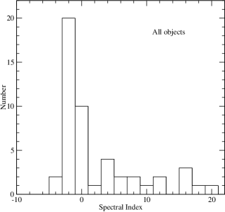
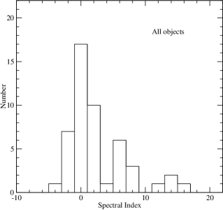
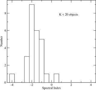
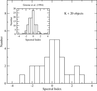
Figure 7: The distributions of the spectral indices for Model I (left) and Model II (right) computed from the flux levels at $K$, $L$, $M$ and $N$ bands ($2.2-10.2~{}\mathrm{\mu m}$) in the SEDs shown in Figure 6. While the upper plots include all 50 objects in our source catalogue (Table 1), the lower plots include only the objects with $K<20$. The distribution for Model II with $K<20$ (lower right) is very similar to that from the observation of the $\rho$ Ophiuchus cloud by Greene et al. (1994) shown in the inset.

3.4 Multi-band far-infrared images

Figure 8 shows simulated images for the SST MIPS bands with central wavelengths ($\lambda_{c}$) at 24, 70 and 160 $\mathrm{\mathrm{\mu m}}$. These are idealised images in which the resolutions are limited only by the number of pixels used in simulations ($500^{2}$ pixels), and are not degraded to the diffraction limit of the SST. The observer is placed at a distance of 140 pc (on the $+z$ axis) from the cluster. At this distance, the images subtend about $15.8\times 15.8\,\mathrm{arcmin}^{2}$. As predicted from the model SEDs (Figure 5), most of the objects appear brighter for Model II in the $24\,\mathrm{\mathrm{\mu m}}$ image because of the warm dust emission from the circumstellar discs. Additional images for Model II with the observers on the $+x$ and $+y$ axis are also computed to create 3-colour, red (160 $\mathrm{\mathrm{\mu m}}$), green (70 $\mathrm{\mathrm{\mu m}}$) and blue (24 $\mathrm{\mathrm{\mu m}}$), composite images. The results are shown in the third row of Figure 2.

Although there is little effect of the circumstellar discs on the predicted SEDs around 70 and 160 $\mathrm{\mu m}$, the presence of the discs influences the morphology of the dust emission. In the lower part of the 70 and 160 $\mathrm{\mu m}$ images of Model II, the ‘butterfly’ structure is caused by an almost edge-on disc. The structure resembles the near infrared images of the edge-on discs around T Tauri stars (e.g. HK Tau C by Stapelfeldt et al. 1998; HH 30 IRS by Burrows et al. 1996) but while these butterflies are formed by scattering, those presented here are the result of thermal processes. Moreover, the scale size of the butterfly structure in the 70 and 160 $\mathrm{\mu m}$ images of Model II is much larger ($\sim 10^{4}$ au) than that seen in the near infrared observations. The typical radius of the circumstellar discs around T Tauri stars based on the near-infrared morphology is order of $\sim 10^{2}$ au (e.g. see Burrows et al. 1996; Lucas & Roche 1998; Stapelfeldt et al. 1998). Interestingly, a recent observation of the T Tauri star ASR 41 in NGC 1333 by Hodapp et al. (2004) showed that the dark band in the reflection nebula around the star can be traced out to $\approx 3000$ au from the centre. Based on their radiative transfer models, they concluded that the large appearance of ASR 41 is probably caused by the shadow of a much smaller disc ($\sim 10^{2}$ au) being projected into the surrounding dusty cloud.

To construct simulated images for actual observations by the SST, the images shown in Figure 8 are degraded to the diffraction limits of an 85 cm telescope; 7.6, 22.1 and 50.4 arcsec for 24, 70, and 160 $\mathrm{\mu m}$ images respectively, by convolving them with a Gaussian filter, and then the image pixels are binned-up to match the pixel scale of MIPS (2.55, 4.99 and 16.0 arcsec for 24, 70, and 160 $\mathrm{\mu m}$ images respectively). The results are shown in Figure 9. The lower flux cut (the minimum value of the flux scale in each image) approximately corresponds to the MIPS limiting flux for each band (0.2, 0.5 and 0.1 MJy sr^-1 for 24, 70 and 160 $\mathrm{\mu m}$ bands respectively). There is no significant change seen in the 24 $\mathrm{\mu m}$ images from the previous images while the 70, and 160 $\mathrm{\mu m}$ images are clearly degraded in resolution and sensitivity. No clear distinction can be made between the two models (with or without the small scale discs) from the 70 $\mathrm{\mu m}$ images. The major structures in the 160 $\mathrm{\mu m}$ images appear to be the same in both models, but the emission from the isolated small structure in the lower half of the images is much weaker in Model II. According to the simulated 24 $\mathrm{\mu m}$ images, 8 and 18 (out of 50) objects are detected above the flux limit for Models I and II, respectively. The simulated images at 70 and 160 $\mathrm{\mu m}$ show cloud structures with surface brightnesses that are 10–100 times the SST detection limits.

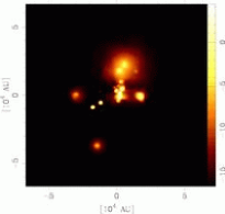
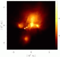
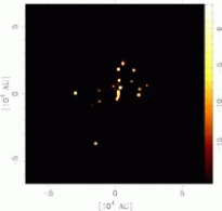
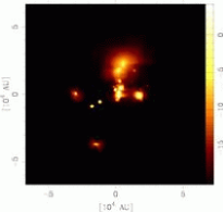
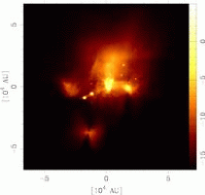
Figure 8: Top: Idealised images for Model I at SST MIPS 24, 70, and 160 $\mathrm{\mu m}$ bands from left to right. Bottom: Same as the top images, but for Model II. The units used for the colour scale in the figures are log of $\mathrm{MJy~{}sr^{-1}}$. The cluster is placed at 140 pc from the observer, and the corresponding angular size of the images is $15.8\times 15.8~{}\mathrm{arcmin^{2}}$. Most of the objects appear brighter in the Model II images due to the warm dust emission from the circumstellar discs. The presence of the disc influences the morphology of the dust emission in the 70 and 160 $\mathrm{\mu m}$ images. The butterfly structures caused by the almost edge-on disc can be seen in the lower part of the 70 and 160 $\mathrm{\mu m}$ images for Model II.

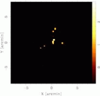
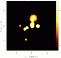
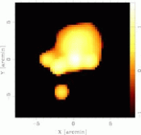
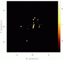
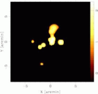
Figure 9: Top: Simulated SST MIPS images for Model I at 24, 70, and 160 $\mathrm{\mu m}$ bands from left to right. Bottom: Same as the top images, but for Model II. As in Figure 8, the colour scale values are in log of $\mathrm{MJy~{}sr^{-1}}$. The images are degraded to the diffraction limits, 7.6, 22.1 and 50.4 arcsec for 24, 70, and 160 $\mathrm{\mu m}$ images respectively, by convolving them with a Gaussian filter. Further, the image pixels are combined to match the instrument resolutions of MIPS (2.55, 4.99 and 16.0 arcsec for 24, 70, and 160 $\mathrm{\mu m}$ images respectively). The lower flux cut (the minimum value of the flux scale in each image) approximately corresponds to the MIPS limiting fluxes (0.2, 0.5 and 0.1 MJy ^-1 for 24, 70 and 160 $\mathrm{\mu m}$ bands respectively). No clear distinction can be made between the two models at 70 and 160 $\mathrm{\mu m}$. The dust emission from the circumstellar disc affects the number of observable stars in the $24~{}\mathrm{\mu m}$ images.

3.5 HKL and SST colour-colour diagrams

Using the flux levels measured in the SEDs shown in Figure 6, we have constructed simulated HKL and SST IRAC (3.6, 4.5 and 5.8 $\mathrm{\mu m}$) colour-colour diagrams, and placed the results in Figures 10 and 11. We have also computed the intrinsic (de-reddened) colours of the objects in Model I and Model II by computing the SEDs without the ISM absorption (i.e. the opacity of the foreground dust is set to zero). The results are shown in the same figure for a comparison. For the HKL colour-colour diagram, only the objects with $K<20$ have been chosen, in order to simulate a deep photometric observation. On the other hand, the objects with a flux greater than $10\,\mathrm{\mu Jy}$ (at $8\,\mathrm{\mu m}$) are used to construct the SST IRAC colour-colour diagram.

As we can see from the left-hand plot in Figure 10, the objects with circumstellar discs (Model II) are not well separated from those without discs (Model I), although the disc objects tend to be slightly redder than the discless objects. This can be understood from the SEDs presented in Figure 5 which shows no significant difference between the flux levels of Model I and Model II in the 1–3 $\mathrm{\mu m}$ wavelength range. The intrinsic HKL colours are less scattered on the diagram. The disc objects seem to lie along the locus of classical T Tauri stars given by Meyer, Calvet, & Hillenbrand (1997):

$$\left(H-K\right)=a\,\left(K-L\right)+b$$

where $a=0.69\left(\pm 0.05\right)$ and $b=-0.05\left(\pm 0.04\right)$. The least-squares fit of our disc object colours gives $a=0.51\left(\pm 0.27\right)$ and $b=-0.11\left(\pm 0.37\right)$ which are in very good agreement with the locus of Meyer et al. (1997). This also indicates our disc SED models are reasonable.

The disc objects and discless objects are well separated in the colour-colour diagram of the SST IRAC bands (in the left plot of Figure 11). Again, this can be roughly explained from the SEDs in Figure 5. The SEDs from Model I and Model II start separating from each other around $\lambda=\mathrm{3\,\mu m}$, and the difference between the flux levels increases as the wavelength increases until it reaches about 10 $\mathrm{\mu m}$. Moreover, the flux level of Model I decreases as a function of the wavelength and vice versa for that of Model II, in this wavelength range (3–10 $\mathrm{\mu m}$). The least-squares fit of the discless objects in the left plot of Figure 11 gives:

$$\left(\log_{10}F_{4.5}-\log_{10}F_{3.6}\right)=a\,\left(\log_{10}F_{5.8}-\log_{10}F_{4.5}\right)+b$$

where $a=1.36\left(\pm 0.14\right)$ and $b=0.20\left(\pm 0.04\right)$. About 85 per cent of the disc objects are located to the right of this fit line.

The intrinsic (de-reddened) colours of the objects are computed in the same way as was done for the HKL colours, and the results are placed in the right-hand plot of Figure 11. The least-squares fit of the disc objects is also shown in the same plot (and also in the left-hand plot). The slope and the intercept of the line are $a=0.78\left(\pm 0.50\right)$ and $b=-0.04\left(\pm 0.05\right)$ respectively. While most of the disc objects are located above $\left(\log_{10}F_{5.8}-\log_{10}F_{4.5}\right)=-0.29$ and along the fit line, the discless objects are located below $\left(\log_{10}F_{5.8}-\log_{10}F_{4.5}\right)=-0.29$ and along the same fit line.

Observers (e.g. Aspin & Barsony 1994; Lada et al. 2000; Muench et al. 2001) often use the JHK or HKL colour-colour diagrams (either J-H vs H-K or H-K vs K-L) to find candidates for young stars or brown dwarfs with accretion discs. As we have seen in this section, a better diagnostic for identifying objects with accretion discs is to use mid-infrared colours (e.g. SST IRAC bands) instead of the near-infrared colours. This may not be true for a more massive cluster since the massive stars could produce a larger fraction of high temperature dust.

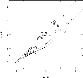
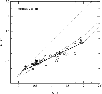
Figure 10: The H-K vs. K-L colour-colour diagrams for the discless objects from Model I (stars) and the disc objects from Model II (circles). The left plot shows the colours of objects (with $K<20$) computed from the SEDs given in Figure 6, and the right plot shows the intrinsic (de-reddened) colours of the same objects. The loci of intrinsic colours for the main-sequence stars (solid line), the giants (dashed line), and the classical T Tauri stars (dash-dot line) from Meyer, Calvet, & Hillenbrand (1997) are also shown along with the reddening vectors (dotted lines) extending to the upper right from the edges of the loci. The least-squares fit of the intrinsic colours of the disc objects (Model II) are shown in thick solid line (right plot).

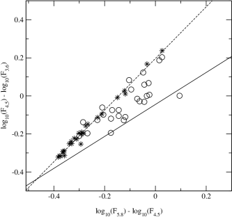
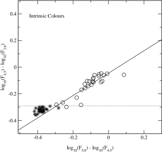
Figure 11: The simulated SST (IRAC) colour-colour diagrams of the discless objects from Model I (stars) and the disc objects from Model II (circles). The $\log_{10}$ of the fluxes at 3.6, 4.5 and 5.8 $\mathrm{\mu m}$ are used here instead of magnitudes. The left plot shows the colours of objects (with $F_{8}>10~{}\mathrm{\mu Jy}$) computed from the SEDs given in Figure 6, along with the least-squares fit line of discless objects (dashed line). About 85 per cent of the disc objects are located to the right of this line. The right plot shows the intrinsic (de-reddened) colours of the same objects along with the least-squares fit (solid line) of the disc objects. The fit (solid line) is also shown in the left plot. While most of the disc objects are located above $\log_{10}F_{5.8}-\log_{10}F_{4.5}=-0.29$ (dotted line) and along the fit line, the discless objects are located below $\log_{10}F_{5.8}-\log_{10}F_{4.5}=-0.29$ and along the same fit line.

4 Conclusions

We have presented three-dimensional Monte Carlo radiative transfer models of a very young low-mass stellar cluster with multiple light sources (23 stars and 27 brown dwarfs). The density structure and the stellar distributions from the large-scale SPH simulation of Bate et al. (2003) were mapped onto our radiative transfer grid without loss of resolution using an AMR grid. The temperature of the ISM and the circumstellar dust was computed using the Monte Carlo radiative equilibrium method of Lucy (1999). The results have been used to compute the SEDs, the far-infrared SST (MIPS bands) images, and the colour-colour diagrams of this cluster.

We find that the presence of circumstellar discs on scales less than 10 au (Model II) influences the morphology of the temperature structure of the cluster (Figure 3), and can affect the temperature of the dust on large scales (up to a several $10^{4}$ au). The dust shadowed by accretion discs has a lower temperature than the model without the discs (Model I). The radiation coming from within a few au of the light sources is anisotropic/bipolar because of the circumstellar discs.

The cluster SEDs (Figure 5) from Models I and II both show peaks around $2\,\mathrm{\mu m}$ and $200\,\mathrm{\mu m}$. The first peak corresponds to that of stellar emission, and the latter corresponds to emission from ISM dust with $T\approx 20\,\mathrm{K}$. The excess emission of Model II between $\lambda=$ 3–30 $\mathrm{\mu m}$ is due to warm dust in the accretion discs. The excess emission in the far infrared ($\lambda>500\,\mathrm{\mu m}$) seen in Model II is caused by the colder ($T<20\,\mathrm{K}$) dust.

Assuming the distance to the cluster to be 140 pc, we have constructed simulated images (Figure 9) for a SST MIPS (24, 70, and 160 $\mathrm{\mu m}$) observation using the appropriate diffraction limits, the sensitivity limits and the angular sizes of pixels. The emission at 24 $\mathrm{\mu m}$ traces the locations of the stars and brown dwarfs very well. No clear distinction can be made between the 70 $\mathrm{\mu m}$ image from Model I and Model II. The major structures in the 160 $\mathrm{\mu m}$ images appear to be same in both Models, but the emission from the isolated small structure in the lower half of the images is much weaker in Model II. In the simulated 24 $\mathrm{\mu m}$ images, 8 out of 50 objects are detected above the flux limit for Model I, and 18 out of 50 objects are detected for Model II. We note that 15 of the 27 brown dwarfs in the cluster (Model II) have $K<20$ and would therefore detectable via deep imaging, while those that are too faint tend to be the youngest, most deeply embedded sources.

Using the flux levels between 2.2 $\mathrm{\mu m}$ and 10 $\mathrm{\mu m}$, the spectral indices of each SEDs were computed. The objects were then classified according to the spectral index values and the ratio of $\log\lambda F_{\lambda}$ values at $\lambda=160\,\mathrm{\mu m}$ (SST MIPS) and at $\lambda=2.2\,\mathrm{\mu m}$ ($K$ band). We have found that 54 per cent of the objects are classified as Class 0, none as Class I, none as flat spectrum, 22 per cent as Class II and 24 per cent as Class III for Model I. For Model II, 56 per cent of objects are classified as Class 0, 18 per cent as Class I, 8 per cent as flat spectrum, 12 per cent as Class II, and 6 per cent as Class III. We also found that the spectral index distribution of Model II ( with $K<20$ objects) is very similar to that of the $\rho$ Ophiuchus cloud observation by Greene et al. (1994). Even though our objects are $0.07\,\mathrm{Myr}$ old, there are a mixture of Class 0–III objects; hence, the class does not necessary relate to the ages of YSOs.

According to the simulated HKL and mid-infrared (SST IRAC) colour-colour diagrams (Figures 10 and 11), the disc objects (Model II) tend to be slightly redder than discless objects (Model I) in the H-K vs K-L diagram, but the two populations are not well separated. This can be understood from the model cluster SEDs (Figure 5) that show no significant difference in the flux levels between $\lambda=$ 1–3 $\mathrm{\mu m}$. On the other hand, the disc objects and discless objects are clearly separated in the colour-colour diagram of the SST IRAC bands (Figure 11). As expected, we find that longer wavelengths are more efficient in detecting circumstellar discs. For example mid-infrared ($\lambda=$ 3–10 $\mathrm{\mu m}$) colours (e.g. SST IRAC bands) are superior to HKL colours. We find that the intrinsic colours of the disc objects (Figure 11) show a distribution very similar to that found by Meyer et al. (1997).

The work presented in this paper can be extended to study how the observable quantities (e.g. colours of stars in a young cluster) evolves with time, by performing radiative transfer model calculations with density structures from a hydrodynamics calculation at different times (ages). Growth of dust grain sizes in accretion discs may become important in predicting how the colours of objects evolve (e.g. see Hansen & Travis 1974; Wood et al. 2002a).

One of the obvious next steps in modelling star formation is to combine SPH and radiative-transfer in order to more accurately predict the temperature of the dust. It is interesting to note that the computational expense of the radiative equilibrium calculation performed here on one SPH time-slice (2400 CPU hours on UKAFF) is a significant fraction of that required to perform the complete SPH simulation (95 000 CPU hours on the same machine) which involves may thousands of time steps. Although it is not immediately clear how often the temperature would have to be computed during a hydrodynamic simulation (the radiative-transfer calculation would have its own Courant condition), it is apparent that a much more efficient method for calculating the radiation transfer is required before a combined SPH/radiative-transfer simulation becomes tractable.

Table 1: Source catalogue

Obj.∗	$M^{*}$	$L^{**}$	$T_{\mathrm{{eff}}}^{**}$	$R^{\dagger}$	$A_{V}$	$K^{\ddagger}$	$F_{8.0}^{\ddagger}$	$F_{24}^{\ddagger}$	$a^{\ddagger}$	$\mathrm{Class^{\ddagger}}$	$A_{V}$	$K^{\ddagger}$	$F_{8.0}^{\ddagger}$	$F_{24}^{\ddagger}$	$a^{\ddagger}$	$\mathrm{Class^{\ddagger}}$	$i$
	$\left[\mathrm{M_{\sun}}\right]$	$\left[\mathrm{L_{\sun}}\right]$	$\left[K\right]$	$\left[\mathrm{R_{\sun}}\right]$			$\left[\mathrm{Jy}\right]$	$\left[\mathrm{Jy}\right]$					$\left[\mathrm{Jy}\right]$	$\left[\mathrm{Jy}\right]$			$\left[\mathrm{deg.}\right]$
					Model I	…	…	…	…	…	Model II	…	…	…	…	…	…
1	0.303	1.002	3740	2.4	3	8	$5.8\times 10^{-2}$	$8.2\times 10^{-3}$	$-2.4$	III	20000	11	$1.4\times 10^{-2}$	$6.3\times 10^{-1}$	$-0.7$	II	86
2	0.211	0.451	3380	2.0	100	10	$1.4\times 10^{-2}$	$5.5\times 10^{0}$	$-1.8$	III	14000	13	$7.5\times 10^{-3}$	$1.9\times 10^{0}$	$0.1$	flat	87
3	0.731	4.134	4610	3.2	20000	17	$1.2\times 10^{-2}$	$3.5\times 10^{-2}$	$0.7$	0	20000	17	$2.5\times 10^{-4}$	$6.4\times 10^{-2}$	0.1	0	13
4	0.162	0.273	3200	1.7	67	16	$2.1\times 10^{-3}$	$7.7\times 10^{-4}$	$-0.7$	II	67	17	$1.8\times 10^{-2}$	$3.1\times 10^{-1}$	$1.8$	I	53
5	0.012	0.004	2510	0.31	180	21	$3.1\times 10^{-5}$	$4.8\times 10^{-5}$	$-0.7$	0	970	21	$8.4\times 10^{-5}$	$2.0\times 10^{-2}$	$0.6$	0	86
6	0.015	0.005	2540	0.36	66	20	$7.6\times 10^{-5}$	$9.1\times 10^{-2}$	$-0.2$	0	2500	19	$4.7\times 10^{-3}$	$2.9\times 10^{-1}$	$2.8$	0	88
7	0.536	2.702	4360	2.9	4	9	$8.7\times 10^{-2}$	$2.3\times 10^{-1}$	$-2.2$	III	4	9	$1.2\times 10^{0}$	$9.1\times 10^{-1}$	$0.4$	I	38
8	0.236	0.560	3460	2.1	4	9	$8.7\times 10^{-2}$	$2.3\times 10^{-1}$	$-2.2$	III	4	10	$1.1\times 10^{0}$	$1.0\times 10^{0}$	$1.1$	I	22
9	0.159	0.264	3180	1.7	7	10	$2.0\times 10^{-2}$	$2.9\times 10^{-3}$	$-2.2$	III	7	10	$4.7\times 10^{-1}$	$2.3\times 10^{0}$	$0.6$	I	63
10	0.413	1.888	4090	2.7	20000	9	$7.6\times 10^{-2}$	$3.3\times 10^{-2}$	$-2.1$	III	20000	9	$7.3\times 10^{-2}$	$6.7\times 10^{-2}$	$-2.1$	III	16
11	0.260	0.690	3550	2.2	11000	21	$4.5\times 10^{-7}$	$2.0\times 10^{-3}$	$-4.1$	0	11000	22	$2.0\times 10^{-7}$	$1.2\times 10^{-3}$	$-3.6$	0	48
12	0.202	0.417	3360	1.9	2	10	$1.7\times 10^{-2}$	$2.3\times 10^{-3}$	$-2.3$	III	2	10	$1.1\times 10^{-1}$	$7.0\times 10^{-1}$	$-0.4$	II	52
13	0.025	0.011	2590	0.52	160	14	$4.5\times 10^{-4}$	$7.9\times 10^{-5}$	$-2.3$	III	160	14	$1.8\times 10^{-3}$	$1.4\times 10^{-2}$	$-1.6$	III	25
14	0.032	0.018	2610	0.65	2	13	$1.4\times 10^{-3}$	$2.2\times 10^{-4}$	$-2.2$	III	2	12	$3.2\times 10^{-2}$	$4.3\times 10^{-2}$	$-0.1$	flat	62
15	0.007	0.002	2470	0.24	19	15	$2.6\times 10^{-4}$	$1.0\times 10^{-4}$	$-2.0$	III	460	15	$1.6\times 10^{-3}$	$3.6\times 10^{-3}$	$-0.0$	flat	86
16	0.012	0.003	2510	0.30	18	16	$3.5\times 10^{-4}$	$6.7\times 10^{-5}$	$-1.4$	II	18	15	$8.2\times 10^{-3}$	$8.2\times 10^{-3}$	1.0	I	43
17	0.008	0.002	2480	0.25	19	16	$2.3\times 10^{-4}$	$4.5\times 10^{-5}$	$-1.4$	II	19	16	$5.4\times 10^{-3}$	$7.1\times 10^{-3}$	$0.7$	I	72
18	0.008	0.002	2480	0.26	6	15	$3.0\times 10^{-4}$	$2.9\times 10^{-3}$	$-1.8$	III	6	11	$1.8\times 10^{-1}$	$1.4\times 10^{-1}$	$0.6$	I	34
19	0.121	0.155	2930	1.5	30	11	$1.6\times 10^{-2}$	$5.6\times 10^{-1}$	$-1.9$	III	30	11	$9.9\times 10^{-2}$	$1.7\times 10^{0}$	$-0.2$	flat	53
20	0.348	1.381	3910	2.6	4600	12	$3.6\times 10^{-2}$	$1.1\times 10^{-2}$	$-1.1$	II	4600	12	$3.4\times 10^{-2}$	$8.5\times 10^{-3}$	$-1.0$	II	68
21	0.069	0.066	2670	1.2	30	15	$2.2\times 10^{-3}$	$1.6\times 10^{-1}$	$-1.0$	II	31	15	$5.3\times 10^{-2}$	$3.4\times 10^{-1}$	$1.4$	I	71
22	0.114	0.140	2880	1.5	4600	14	$4.7\times 10^{-3}$	$3.9\times 10^{-3}$	$-1.0$	II	4600	14	$5.0\times 10^{-3}$	$1.8\times 10^{-3}$	$-1.0$	II	70
23	0.032	0.018	2610	0.67	1000	44	$5.0\times 10^{-10}$	$7.0\times 10^{-3}$	$8.7$	0	1100	45	$7.7\times 10^{-8}$	$1.5\times 10^{-3}$	$7.5$	0	79
24	0.173	0.310	3250	1.8	990	33	$1.6\times 10^{-8}$	$1.5\times 10^{-2}$	$4.1$	0	990	43	$1.1\times 10^{-9}$	$2.6\times 10^{-3}$	$5.5$	0	78
25	0.229	0.525	3440	2.0	5200	33	$2.4\times 10^{-7}$	$2.4\times 10^{-3}$	$4.0$	0	5200	45	$1.1\times 10^{-9}$	$1.1\times 10^{-3}$	$5.5$	0	52
26	0.133	0.185	3010	1.6	4700	35	$6.3\times 10^{-8}$	$9.0\times 10^{-2}$	$7.1$	0	8000	46	$3.8\times 10^{-11}$	$7.8\times 10^{-4}$	$3.5$	0	85
27	0.005	0.002	2460	0.22	220	27	$6.3\times 10^{-7}$	$3.6\times 10^{-4}$	$0.0$	0	220	30	$6.8\times 10^{-8}$	$1.6\times 10^{-5}$	$0.7$	0	30
28	0.017	0.006	2550	0.38	1300	21	$2.4\times 10^{-6}$	$2.1\times 10^{-5}$	$-2.7$	0	1300	19	$3.0\times 10^{-5}$	$3.1\times 10^{-6}$	$-1.9$	III	80
29	0.058	0.050	2650	1.1	340	18	$4.1\times 10^{-6}$	$2.9\times 10^{-2}$	$-3.9$	0	340	19	$5.1\times 10^{-6}$	$1.8\times 10^{-2}$	$-3.0$	0	61
30	0.069	0.065	2670	1.2	37	15	$1.9\times 10^{-4}$	$2.9\times 10^{-3}$	$-0.8$	II	37	17	$1.7\times 10^{-2}$	$4.6\times 10^{-1}$	$2.7$	0	58
31	0.023	0.010	2590	0.50	120	17	$3.2\times 10^{-4}$	$1.4\times 10^{-1}$	$-0.8$	0	120	17	$5.6\times 10^{-2}$	$3.7\times 10^{-1}$	$2.7$	0	74
32	0.239	0.571	3470	2.1	22000	21	$2.2\times 10^{-3}$	$4.2\times 10^{-2}$	$1.9$	0	22000	21	$2.3\times 10^{-3}$	$2.6\times 10^{-2}$	$1.8$	0	65
33	0.087	0.093	2720	1.4	310	32	$2.6\times 10^{-6}$	$5.3\times 10^{-3}$	$3.5$	0	310	34	$3.1\times 10^{-6}$	$3.2\times 10^{-3}$	$5.7$	0	77
34	0.047	0.035	2630	0.90	21	14	$1.6\times 10^{-3}$	$2.5\times 10^{-2}$	$-1.4$	II	7400	17	$1.9\times 10^{-4}$	$6.2\times 10^{-2}$	$0.4$	0	89
35	0.083	0.086	2710	1.3	51000	13	$3.8\times 10^{-3}$	$2.3\times 10^{-2}$	$-1.4$	II	51000	16	$6.3\times 10^{-4}$	$7.7\times 10^{-2}$	$-0.3$	II	66
36	0.044	0.032	2630	0.86	15	14	$1.7\times 10^{-3}$	$6.0\times 10^{-1}$	$-1.4$	II	15	14	$4.4\times 10^{-2}$	$2.6\times 10^{-1}$	$1.0$	I	75
37	0.022	0.009	2580	0.47	820	15	$4.4\times 10^{-4}$	$1.9\times 10^{-3}$	$-1.6$	II	820	15	$4.4\times 10^{-4}$	$5.5\times 10^{-4}$	$-1.6$	II	44
38	0.079	0.081	2690	1.3	3300	41	$2.3\times 10^{-9}$	$3.9\times 10^{-3}$	$5.0$	0	3300	53	$1.3\times 10^{-6}$	$2.3\times 10^{-3}$	$15.7$	0	61
39	0.070	0.066	2670	1.2	450	50	$1.8\times 10^{-7}$	$8.4\times 10^{-2}$	$15.4$	0	450	64	$5.0\times 10^{-11}$	$2.9\times 10^{-4}$	$14.1$	0	78
40	0.039	0.025	2620	0.77	1000	51	$1.1\times 10^{-7}$	$5.8\times 10^{-2}$	$16.0$	0	1000	61	$5.9\times 10^{-11}$	$8.9\times 10^{-6}$	$12.0$	0	60
41	0.047	0.035	2630	0.90	1400	79	$6.3\times 10^{-8}$	$8.1\times 10^{-2}$	$32.1$	0	1400	64	$4.0\times 10^{-11}$	$1.2\times 10^{-3}$	$14.4$	0	63
42	0.095	0.106	2760	1.4	2300	50	$2.3\times 10^{-7}$	$3.7\times 10^{-2}$	$15.1$	0	2300	35	$1.2\times 10^{-7}$	$2.3\times 10^{-2}$	$5.8$	0	76
43	0.022	0.009	2580	0.48	580	49	$1.4\times 10^{-9}$	$4.1\times 10^{-3}$	$9.7$	0	580	40	$1.2\times 10^{-6}$	$1.9\times 10^{-3}$	$8.5$	0	77
44	0.102	0.118	2800	1.5	2700	53	$2.5\times 10^{-6}$	$2.4\times 10^{-2}$	$17.4$	0	2700	37	$4.1\times 10^{-7}$	$1.5\times 10^{-2}$	$6.2$	0	68
45	0.083	0.087	2710	1.3	3800	69	$6.0\times 10^{-13}$	$4.2\times 10^{-3}$	$21.0$	0	3800	36	$1.4\times 10^{-6}$	$2.3\times 10^{-3}$	$6.9$	0	66
46	0.031	0.017	2610	0.64	1100	39	$2.4\times 10^{-9}$	$1.1\times 10^{-3}$	$5.1$	0	6100	44	$8.4\times 10^{-11}$	$1.6\times 10^{-8}$	$0.6$	0	89
47	0.035	0.021	2620	0.70	1800	34	$2.0\times 10^{-9}$	$4.1\times 10^{-4}$	$0.2$	0	6100	35	$3.1\times 10^{-8}$	$5.0\times 10^{-4}$	$2.5$	0	87
48	0.029	0.015	2610	0.60	1100	50	$1.9\times 10^{-10}$	$1.4\times 10^{-7}$	$6.2$	0	1100	40	$1.8\times 10^{-10}$	$2.6\times 10^{-8}$	1.5	0	56
49	0.013	0.004	2520	0.32	18000	65	$1.4\times 10^{-12}$	$3.5\times 10^{-9}$	$12.9$	0	19000	99	$2.3\times 10^{-16}$	$2.8\times 10^{-8}$	$26.5$	0	88
50	0.008	0.002	2480	0.25	7400	46	$1.2\times 10^{-8}$	$2.7\times 10^{-2}$	$12.9$	0	7400	41	$8.2\times 10^{-9}$	$3.4\times 10^{-2}$	$8.5$	0	63

$\left(*\right)$ From the SPH calculation of Bate et al. (2003).

$\left(**\right)$ Computed (at an age of 1/4 Myrs) from the isochrone data available on http://www.mporzio.astro.it/~dantona/prems.html. See also D’Antona & Mazzitelli (1998).

$\left(\dagger\right)$ Estimated by using the $L$ (column 3) and $T_{\mathrm{eff}}$ (column 4) in the Stefan-Boltzmann law.

$\left(\ddagger\right)$ Based on the SEDs of individual objects computed for an observer on $+z$ axis at 140 pc. See section 3.3.

References

- Adams et al. (1987) Adams F. C., Lada C. J., Shu F. H., 1987, ApJ, 312, 788
- Anders & Grevesse (1989) Anders E., Grevesse N., 1989, Geochim. Cosmochim. Acta, 53, 197
- Andre et al. (1993) Andre P., Ward-Thompson D., Barsony M., 1993, ApJ, 406, 122
- Artymowicz & Lubow (1994) Artymowicz P., Lubow S. H., 1994, ApJ, 421, 651
- Aspin & Barsony (1994) Aspin C., Barsony M., 1994, A&A, 288, 849
- Baraffe et al. (1998) Baraffe I., Chabrier G., Allard F., Hauschildt P. H., 1998, A&A, 337, 403
- Baraffe et al. (2002) —, 2002, A&A, 382, 563
- Bate et al. (2002a) Bate M. R., Bonnell I. A., Bromm V., 2002a, MNRAS, 332, L65
- Bate et al. (2002b) —, 2002b, MNRAS, 336, 705
- Bate et al. (2003) —, 2003, MNRAS, 339, 577
- Beckwith & Sargent (1991) Beckwith S. V. W., Sargent A. I., 1991, ApJ, 381, 250
- Beckwith et al. (1990) Beckwith S. V. W., Sargent A. I., Chini R. S., Guesten R., 1990, AJ, 99, 924
- Bertout et al. (1999) Bertout C., Robichon N., Arenou F., 1999, A&A, 352, 574
- Bjorkman & Wood (2001) Bjorkman J. E., Wood K., 2001, ApJ, 554, 615
- Burrows et al. (1996) Burrows C. J., Stapelfeldt K. R., Watson A. M., Krist J. E., Ballester G. E., Clarke J. T., Hester J. J., Hoessel J. G., Holtzman J. A., Mould J. R., Scowen P. A., Trauger J. T. and Westphal J. A., 1996, ApJ, 473, 437
- Censori & D’Antona (1998) Censori C., D’Antona F., 1998, in ASP Conf. Ser. 134: Brown Dwarfs and Extrasolar Planets, Rebolo R., Martin E. L., Zapatero-Osorio M. R., eds., Astron. Soc. Pac., p. 518
- Chandrasekhar (1960) Chandrasekhar S., 1960, Radiative Transfer. Dover, New York
- Chiang & Goldreich (1997) Chiang E. I., Goldreich P., 1997, ApJ, 490, 368
- Cotera et al. (2001) Cotera A. S., Whitney B. A., Young E., Wolff M. J., Wood K., Povich M., Schneider G., Rieke M., Thompson R., 2001, ApJ, 556, 958
- D’Alessio et al. (1998) D’Alessio P., Canto J., Calvet N., Lizano S., 1998, ApJ, 500, 411
- D’Antona & Mazzitelli (1997) D’Antona F., Mazzitelli I., 1997, in Memorie della Societa Astronomica Italiana, Vol. 68, p. 807
- D’Antona & Mazzitelli (1998) —, 1998, in ASP Conf. Ser. 134: Brown Dwarfs and Extrasolar Planets, Rebolo R., Martin E. L., Zapatero-Osorio M. R., eds.,Astron. Soc. Pac., p. 442
- Draine & Lee (1984) Draine B. T., Lee H. M., 1984, ApJ, 285, 89
- Eisner & Carpenter (2003) Eisner J. A., Carpenter J. M., 2003, ApJ, 598, 1341
- Folini et al. (2003) Folini D., Walder R., Psarros M., Desboeufs A., 2003, in ASP Conf. Ser. 288: Stellar Atmosphere Modeling, Hubeny I., Mihalas D., Werner K., eds., Astron. Soc. Pac., San Francisco, p. 433
- Frank et al. (2002) Frank J., King A., Raine D. J., 2002, Accretion Power in Astrophysics: Third Edition. Cambridge Univ. Press, Cambridge, p. 398
- Greene et al. (1994) Greene T. P., Wilking B. A., Andre P., Young E. T., Lada C. J., 1994, ApJ, 434, 614
- Grevesse & Noels (1993) Grevesse N., Noels A., 1993, in Origin and Evolution of the Elements, Prantzos N., Vangioni-Flam E., Casse M., eds., Cambridge Univ. Press, Cambridge, p. 15
- Haisch et al. (2001) Haisch K. E., Lada E. A., Piña R. K., Telesco C. M., Lada C. J., 2001, AJ, 121, 1512
- Hanner (1988) Hanner M., 1988, in NASA Conf. Pub. 3004, 22, Vol. 3004, p. 22
- Hansen & Travis (1974) Hansen J. E., Travis L. D., 1974, Space Science Reviews, 16, 527
- Harries (2000) Harries T. J., 2000, MNRAS, 315, 722
- Harries et al. (2004) Harries T. J., Monnier J. M., Symington N. H., Kurosawa R., 2004, MNRAS, (in press)
- Henyey & Greenstein (1941) Henyey L. C., Greenstein J. L., 1941, ApJ, 93, 70
- Hillier (1991) Hillier D. J., 1991, A&A, 247, 455
- Hodapp et al. (2004) Hodapp K. W., Walker C. H., Reipurth B., Wood K., Bally J., Whitney B. A., Connelley M., 2004, ApJ, 601, L79
- Ivezić et al. (1999) Ivezić v. Z., Nenkova M., Elitzur M., 1999, User Manual for DUSTY. University of Kentucky Internal Report
- Kenyon et al. (1993) Kenyon S. J., Calvet N., Hartmann L., 1993, ApJ, 414, 676
- Kenyon & Hartmann (1995) Kenyon S. J., Hartmann L., 1995, ApJS, 101, 117
- Kim et al. (1994) Kim S., Martin P. G., Hendry P. D., 1994, ApJ, 422, 164
- Krause et al. (2003) Krause O., Lemke D., Tóth L. V., Klaas U., Haas M., Stickel M., Vavrek R., 2003, A&A, 398, 1007
- Kurosawa & Hillier (2001) Kurosawa R., Hillier D. J., 2001, A&A, 379, 336
- Lada (1987) Lada C. J., 1987, in IAU Symp. 115: Star Forming Regions, Peimbert M., Jugaku J., ed., Kluwer, Dordrecht, p. 1
- Lada et al. (2000) Lada C. J., Muench A. A., Haisch K. E., Lada E. A., Alves J. F., Tollestrup E. V., Willner S. P., 2000, AJ, 120, 3162
- Larson (1981) Larson R. B., 1981, MNRAS, 194, 809
- Lefevre et al. (1982) Lefevre J., Bergeat J., Daniel J.-Y., 1982, A&A, 114, 341
- Liseau et al. (1995) Liseau R., Lorenzetti D., Molinari S., Nisini B., Saraceno P., Spinoglio L., 1995, A&A, 300, 493
- Lucas & Roche (1998) Lucas P. W., Roche P. F., 1998, MNRAS, 299, 723
- Lucy (1999) Lucy L. B., 1999, A&A, 344, 282
- Luhman & Rieke (1999) Luhman K. L., Rieke G. H., 1999, ApJ, 525, 440
- Mathis et al. (1977) Mathis J. S., Rumpl W., Nordsieck K. H., 1977, ApJ, 217, 425
- McCaughrean et al. (1995) McCaughrean M., Zinnecker H., Rayner J., Stauffer J., 1995, in The Bottom of the Main Sequence - and Beyond, Tinney C. G., ed., ESO Astrophysics Symposia, Springer-Verlag, Berlin, p. 209
- Meyer et al. (1997) Meyer M. R., Calvet N., Hillenbrand L. A., 1997, AJ, 114, 288
- Mihalas (1978) Mihalas D., 1978, Stellar atmospheres. 2nd ed.: San Francisco, W. H. Freeman and Co.
- Muench et al. (2001) Muench A. A., Alves J., Lada C. J., Lada E. A., 2001, ApJ, 558, L51
- Myers et al. (1987) Myers P. C., Fuller G. A., Mathieu R. D., Beichman C. A., Benson P. J., Schild R. E., Emerson J. P., 1987, ApJ, 319, 340
- Niccolini et al. (2003) Niccolini G., Woitke P., Lopez B., 2003, A&A, 399, 703
- Ostriker et al. (2001) Ostriker E. C., Stone J. M., Gammie C. F., 2001, ApJ, 546, 980
- Pagani (1998) Pagani L., 1998, A&A, 333, 269
- Pascucci et al. (2004) Pascucci I., Wolf S., Steinacker J., Dullenmonds C. P., Henning Th., Niccolini G., Woitke P., Lopez B., 2004, A&A, (in press)
- Shakura & Sunyaev (1973) Shakura N. I., Sunyaev R. A., 1973, A&A, 24, 337
- Spitzer (1978) Spitzer L., 1978, Physical processes in the interstellar medium. New York Wiley-Interscience
- Stapelfeldt et al. (1998) Stapelfeldt K. R., Krist J. E., Menard F., Bouvier J., Padgett D. L., Burrows C. J., 1998, ApJ, 502, L65
- Steinacker et al. (2002) Steinacker J., Bacmann A., Henning Th., 2002, JQSRT, 75, 765
- Steinacker et al. (2003) Steinacker J., Henning Th., Bacmann A., Semenov D., 2003, A&A, 401, 405
- Stenholm et al. (1991) Stenholm L. G., Störzer H., Wehrse R., 1991, JQSRT, 45, 1, 47
- Symington (2004) Symington N. H., 2004, PhD thesis, Univ. Exeter
- Whitney et al. (2003a) Whitney B. A., Wood K., Bjorkman J. E., Cohen M., 2003a, ApJ, 598, 1079
- Whitney et al. (2003b) Whitney B. A., Wood K., Bjorkman J. E., Wolff M. J., 2003b, ApJ, 591, 1049
- Wilking et al. (1989) Wilking B. A., Lada C. J., Young E. T., 1989, ApJ, 340, 823
- Witt & Gordon (1996) Witt A. N., Gordon K. D., 1996, ApJ, 463, 681
- Wolf et al. (1999) Wolf S., Henning Th., Stecklum B., 1999, A&A, 349, 839
- Wood et al. (2002a) Wood K., Lada C. J., Bjorkman J. E., Kenyon S. J., Whitney B., Wolff M. J., 2002a, ApJ, 567, 1183
- Wood et al. (2002b) Wood K., Wolff M. J., Bjorkman J. E., Whitney B., 2002b, ApJ, 564, 887