High-redshift QSOs in the GOODS

High-redshift QSOs in the GOODS

1 Introduction

QSOs are intrinsically luminous and therefore can be seen rather easily at large distances; but they are rare, and finding them requires surveys over large areas. As a consequence, at present, the number density of QSOs at high redshift is not well known. Recently, the Sloan Digital Sky Survey (SDSS) has produced a breakthrough, discovering QSOs up to $z=6.43$ Fan03 and building a sample of six QSOs with $z>5.7$. The SDSS, however, has provided information only about very luminous QSOs ($M_{1450}\ \raise-2.0pt\hbox{\hbox to0.0pt{\hbox{$\sim$}\hss}\raise 5.0pt\hbox{$<$}\ }-26.5$), leaving unconstrained the faint end of the high-$z$ QSO Luminosity Function (LF), which is particularly important to understand the interplay between the formation of galaxies and super-massive black holes (SMBH) and to measure the QSO contribution to the UV ionizing background Madau99 . New deep multi-wavelength surveys like the Great Observatories Origins Deep Survey (GOODS), described by M.Dickinson, M.Giavalisco and H.Ferguson in this conference, provide significant constraints on the space density of less luminous QSOs at high redshift. Here we present a search for high-$z$ QSOs, identified in the two GOODS fields on the basis of deep imaging in the optical (with HST) and X-ray (with Chandra), and discuss the allowed space density of QSOs in the early universe, updating the results presented in cristiani04 .

2 The Database

The optical data used in this search have been obtained with the ACS onboard HST, as described by M.Giavalisco. Mosaics have been created from the first three epochs of observations, out of a total of five, in the bands $F435W(B_{435})$, $F606W(V_{606})$, $F775W(i_{775})$, $F850LP(z_{850})$. The catalogs used to select high-$z$ QSOs have been generated using the SExtractor software, performing the detection in the $z_{850}$ band and then using the isophotes defined during this process as apertures for photometry in the other bands. This is a common practice avoiding biases due to aperture mismatch coming from independent detections.

The X-ray observations of the HDF-N and CDF-S consist of 2 Ms and 1 Ms exposures, respectively, providing the deepest views of the Universe in the 0.5–8.0 keV band. The X-ray completeness limits over $~{}90\%$ of the area of the GOODS fields are similar, with flux limits (S/N$=5$) of $~{}1.7\times 10^{-16}$ erg cm^-2 s^-1 (0.5–2.0 keV) and $~{}1.2\times 10^{-15}$  erg cm^-2 s^-1 (2–8 keV) in the HDF-N field, and $\approx 2.2\times 10^{-16}$ erg cm^-2 s^-1 (0.5–2.0 keV) and $\approx 1.5\times 10^{-15}$ erg cm^-2 s^-1 (2–8 keV) in the CDF-S field. The sensitivity at the aim point is about 2 and 4 times better for the CDF-S and HDF-N, respectively. As an example, assuming an X-ray spectral slope of $\Gamma=$ 2.0, a source detected with a flux of $1.0\times 10^{-16}$ erg cm^-2 s^-1 would have both observed and rest-frame luminosities of $8\times 10^{42}$ erg s^-1, and $3\times 10^{43}$ erg s^-1 at $z=3$, and $z=5$, respectively (assuming no Galactic absorption). Alexander03 produced point-source catalogs for the HDF-N and CDF-S and Giacconi02 for the CDF-S with more than 1000 detected sources in total.

3 The Selection of the QSO candidates

We have carried out the selection of the QSO candidates in the magnitude interval $22.45<z_{850}<25.25$. Four optical criteria have been tailored on the basis of typical QSO SEDs in order to select QSOs at progressively higher redshift in the interval $3.5\ \raise-2.0pt\hbox{\hbox to0.0pt{\hbox{$\sim$}\hss}\raise 5.0pt\hbox{$<$}\ }z\ \raise-2.0pt\hbox{\hbox to0.0pt{\hbox{$\sim$}\hss}\raise 5.0pt\hbox{$<$}\ }5.2$. The criteria have been applied independently and produced in total $645$ candidates in the CDF-S and $557$ in the HDF-N. They select a broad range of high-$z$ AGN, not limited to broad-lined (type-1) QSOs, and are less stringent than those typically used to identify high-$z$ galaxies. We have checked the criteria against QSOs and galaxies known in the literature within the magnitude and redshift ranges of interest confirming the high completeness of the adopted criteria.

Below $z\simeq 3.5$ the typical QSO colors in the ACS bands move close to the locus of stars and low-redshift galaxies. Beyond $z\simeq 5.2$ the $i-z$ color starts increasing and infrared bands would be needed to identify QSOs efficiently with an “$i$-dropout” technique.

4 Match with Chandra Sources

The optical candidates have been matched with X-ray sources detected by Chandra within an error radius corresponding to the $3~{}\sigma$ X-ray positional uncertainty. With this tolerance the expected number of false matches is five and indeed two misidentifications, i.e. cases in which a brighter optical source lies closer to the X-ray position, have been rejected (both in the CDF-S).

The sample has been reduced in this way to 11 objects in the CDF-S and 6 in the HDF-N. Type-1 QSOs with $M_{1450}<-21$, given the measured dispersion in their optical-to-X-ray flux ratio Vignali03 , are detectable in our X-ray observation up to $z\ \raise-2.0pt\hbox{\hbox to0.0pt{\hbox{$\sim$}\hss}\raise 5.0pt\hbox{$>$}\ }5.2$. Conversely, any $z>3.5$ source in the GOODS region detected in the X-rays must harbor an AGN ($L_{x}(0.5-2~{}{\rm keV})\ \raise-2.0pt\hbox{\hbox to0.0pt{\hbox{$\sim$}\hss}\raise 5.0pt\hbox{$>$}\ }10^{43}~{}{\rm erg~{}s^{-1}}$).

5 Redshifts of the QSO candidates

Twelve objects out of the 17 selected have spectroscopic confirmations. Nine are QSOs with redshifts between $2.6$ and $5.2$. Three are reported to be galaxies, and the relatively large offsets between the X-ray and optical positions suggest that they could be misidentifications. Both quasars of Type I and II are detected.

Photometric redshifts of the 17 QSO candidates have been estimated by comparing with a $\chi^{2}$ technique (see Arnouts99 for details) the observed ACS colors to those expected on the basis of a) the typical QSO SEDs; b) a library of template SEDs of galaxies (the “extended Coleman” of Arnouts99 ). For the nine QSOs with spectroscopic confirmation the photometric redshifts are in good agreement with the observed ones. In general the estimates a) and b) are similar, since the color selection criteria both for galaxies and QSOs rely on a strong flux decrement in the blue part of the spectrum - due to the IGM and possibly an intrinsic Lyman limit absorption - superimposed on an otherwise blue continuum. If we limit ourselves to the redshift range $z>4$ - where the selection criteria and the photometric redshifts are expected to be most complete and reliable - in addition to one spectroscopically confirmed QSO (HDF-N 123647.9+620941, $z=5.186$) we estimate that between 1-2 more QSOs are present in the GOODS, depending on whether galaxy or QSO SEDs are adopted for the photometric redshifts. This brings the total to no more than three QSOs with redshift larger than 4.

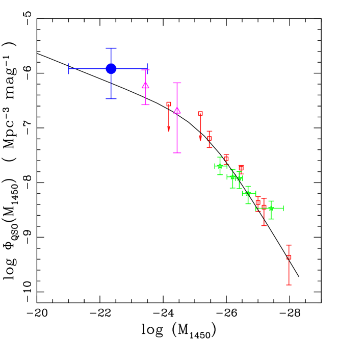
Figure 1: Differential QSO luminosity function at $z\sim 4-5$. Squares: data from Kennefick95 and upper limits from Kennefick96 at $z\sim 4.4$. Stars: SDSS fan01b computed at $3.5<z<5$ assuming a power-law decline and rescaled to $z=4.3$. Triangles: COMBO-17 LF COMBO17 , for $4.2<z<4.8$. Circle: GOODS LF at $4<z<5.2$. The continuous line shows the prediction of the PDE model described in the text. All LFs have been rescaled to a cosmology with $h,\Omega_{\rm tot},\Omega_{m},\Omega_{\Lambda}=0.7,1.0,0.3,0.7$.

6 Comparison with the models

Let us compare now the QSO counts observed in the $z_{850}$ band with two phenomenological and two more physically motivated models. The double power-law fit of the 2QZ QSO LF boyle00 has been extrapolated for $z>2.7$ (the peak of QSO activity) in a way to produce a power-law decrease of the number of bright QSOs by a factor 3.5 per unit redshift interval, consistent with the $3.0^{+1.3}_{-0.9}$ factor found by fan01b for the bright part of the LF. The extrapolation is carried out either as a Pure Luminosity Evolution (PLE) or a Pure Density Evolution (PDE). The PLE model predicts about 17 QSOs with $z_{850}<25.25$ at redshift $z>4$ (27 at $z>3.5$) in the 320 arcmin² of the two GOODS fields, and is inconsistent with the observations at a more than $3\sigma$ level. The PDE estimate is 2.9 QSOs at $z>4$ (6.7 at $z>3.5$).

It is possible to connect QSOs with dark matter halos (DMH) formed in hierarchical cosmologies with a minimal set of assumptions (MIN model, e.g. haiman01 ): a) QSOs are hosted in newly formed halos with b) a constant SMBH/DMH mass ratio $\epsilon$ and c) accretion at the Eddington rate. The bolometric LF of QSOs is then expressed by:

$$\Phi(L|z)dL=n_{\rm PS}(M_{H}|z)\int_{t(z)-t_{\rm duty}}^{t(z)}\hskip-31.29802ptP(t_{f}|M_{H},t(z))dt_{f}\epsilon^{-1}{{dL}\over{L_{\rm Edd}}}$$ (1)

where the abundance of DMHs of mass $M_{H}$ is computed using the Press & Schechter ps74 recipe, the distribution $P(t_{f}|M_{H},t(z))dt_{f}$ of the formation times $t_{f}$ follows lc93 , $t_{\rm duty}$ is the QSO duty cycle and $L_{Edd}=10^{4.53}~{}L_{\odot}$ is the Eddington luminosity of a $1\ M_{\odot}$ SMBH. This model is known to overproduce the number of high-$z$ QSOs haiman99 and in the present case predicts $151$ QSOs at $z>4$ ($189$ at $z>3.5$).

To cure the problems of the MIN model feedback effects have been invoked, for example assuming that the QSOs shine a $t_{\rm delay}$ time after DMH formation (DEL model; Monaco00 , granato01 . The QSO LF is then computed at a redshift $z^{\prime}$ corresponding to $t(z)-t_{\rm delay}$. The predictions of the DEL model are very close to the PDE, with $3.2$ QSOs expected at $z>4$ ($4.8$ at $z>3.5$), in agreement with the observations. While all the models presented here are consistent with the recent QSO LF measurement of the COMBO-17 survey COMBO17 at $z\simeq 2-3$, only the PDE and DEL models fit the COMBO-17 LF in the range $4.2<z<4.8$ and $M_{1450}<-26$.

7 Conclusions

At $z>4$ the space density of moderate luminosity ($M_{1450}\simeq-23$) QSOs is significantly lower than the prediction of simple recipes matched to the SDSS data, such as a PLE evolution of the LF or a constant universal efficiency in the formation of SMBH in DMH. A flattening of the observed high-$z$ LF is required below the typical luminosity regime ($M_{1450}\ \raise-2.0pt\hbox{\hbox to0.0pt{\hbox{$\sim$}\hss}\raise 5.0pt\hbox{$<$}\ }-26.5$) probed by the SDSS. An independent indication that this flattening must occur comes from the statistics of bright lensed QSOs observed in the SDSS Wyithe02 that would be much larger if the LF remains steep in the faint end. A similar result has been obtained at $5\ \raise-2.0pt\hbox{\hbox to0.0pt{\hbox{$\sim$}\hss}\raise 5.0pt\hbox{$<$}\ }z\ \raise-2.0pt\hbox{\hbox to0.0pt{\hbox{$\sim$}\hss}\raise 5.0pt\hbox{$<$}\ }6.5$, by Barger03 . The QSO contribution to the UV background is insufficient to ionize the IGM at these redshifts. This is an indication that at these early epochs the formation or the feeding of SMBH is strongly suppressed in relatively low-mass DMH, as a consequence of feedback from star formation granato01 and/or photoionization heating of the gas by the UV background haiman99 , accomplishing a kind of inverse hierarchical scenario.

References

- (1) Alexander, D.M., et al. 2003, AJ 126, 539
- (2) Arnouts, S., Cristiani, S., Moscardini, L., Matarrese, S., Lucchin, F., Fontana, A., Giallongo, E., 1999, MNRAS 310, 540
- (3) Barger, A.J., Cowie, L.L., Richards, E.A., 2000, AJ 119, 2092
- (4) Barger, A.J., Cowie, L.L., Capak, P., Alexander, D.M., Bauer, F.E., Brandt, W.N., Garmire, G.P., Hornschemeier, A.E., 2003, ApJ 584, L61
- (5) Boyle, B.J.,Shanks, T., Croom, S.M., Smith, R.J., Miller, L., Loaring, N., & Heymans, C., 2000, MNRAS 317, 1014
- (6) Cristiani, S., et al. 2004, ApJ 600, L119
- (7) Fan, X., Strauss, M.A., Schneider, D., et al., 2001, AJ 121,54
- (8) Fan, X., Strauss, M.A., Schneider, D.P., Becker, R.H., et al., 2003, AJ 125, 1649
- (9) Giacconi, R., et al. 2002, ApJS 139, 369, G02
- (10) Granato, G.L., Silva, L., Monaco, P., Panuzzo, P., Salucci, P., De Zotti, G., Danese, L., 2001, MNRAS 324, 757
- (11) Haiman, Z., & Hui, L., 2001, ApJ 547, 27
- (12) Haiman, Z., Madau, P., & Loeb, A., 1999, ApJ 514, 535
- (13) Kennefick, J.D., Djorgovski, S.G., & de Carvalho, 1995, AJ 110, 2553
- (14) Kennefick, J.D., Djorgovski, S.G., & Meylan, G., 1996, AJ 11, 1816
- (15) Lacey, C., & Cole, S., 1993, MNRAS 262, 627
- (16) Madau, P., Haardt, F., Rees, M.J., 1999, ApJ 514, 648
- (17) Monaco, P., Salucci, P., Danese, L., 2000, MNRAS 311, 279
- (18) Press, W.H., & Schechter, P., 1974, ApJ 187, 425
- (19) Vignali, C., et al. 2003, AJ 125, 2876
- (20) Wolf, C., Wisotzki, L., Borch, A., Dye, S., Kleinheinrich, M., Meisenheimer, K., 2003, A&A 408, 499
- (21) Wyithe, J.S.B., Loeb, A., 2002, ApJ 577, 57