Antenna Instrumental Polarization and its Effects on $E$- and $B$-Modes for CMBP Observations

We analyze the instrumental polarization generated by the antenna system (optics and feed horn) due to the unpolarized sky emission. Our equations show that it is given by the convolution of the unpolarized emission map $T_{b}(\theta,\phi)$ with a sort of instrumental polarization beam $\Pi$ defined by the co- and cross-polar patterns of the antenna. This result is general, it can be applied to all antenna systems and is valid for all schemes to detect polarization, like correlation and differential polarimeters. The axisymmetric case is attractive: it generates an $E$-mode–like $\Pi$ pattern, the contamination does not depend on the scanning strategy and the instrumental polarization map does not have $B$-mode contamination, making axisymmetric systems suitable to detect the faint $B$-mode signal of the Cosmic Microwave Background Polarization. The $E$-mode of the contamination only affects the FWHM scales leaving the larger ones significantly cleaner. Our analysis is also applied to the SPOrt experiment where we find that the contamination of the $E$-mode is negligible in the $\ell$-range of interest for CMBP large angular scale investigations (multipole $\ell<10$).

1 Introduction

The Polarization of the Cosmic Microwave Background (CMBP) represents a powerful tool to determine cosmological parameters, investigate the epoch of the formation of the first galaxies and have an insight into the inflationary era (e.g. see Zaldarriaga, Spergel & Seljak 1997, Kamionkowski & Kosowsky 1998).

In spite of its importance the CMBP signal is weak: The $E$-mode component is about 1-10% of the already faint CMB anisotropy, depending on the angular scale; The $B$-mode is even weaker, with an emission level that can be more than 3 orders of magnitude below the anisotropy, depending on the tensor-to-scalar perturbation ratio $T/S$ (e.g. see Kamionkowski & Kosowsky 1998).

The investigation of CMBP is at the beginning with a first detection of the $E$-mode claimed by the DASI team (Kovac et al. 2002) and a first measurement of the TE cross-spectrum provided by the WMAP team (Kogut et al. 2003). Anyway, we are far from a full characterization of the $E$-mode and the $B$-mode is still elusive.

In this frame it is important to deal with instruments with low contamination, expecially in the $B$ component, for which even a 0.1% leakage from the Temperature anisotropy might wash out any detection. One should also note that the contamination from the anisotropy term is not easily removed by destriping techniques, its level being not constant over the scans performed to observe the sky (e.g. see Revenu et al. 2000, Sbarra et al. 2003 and references therein for descriptions of destriping techniques), so that a clean instrument is necessary to avoid complex data reductions.

A clear understanding of the contamination from the unpolarized background introduced by the instrument itself is thus mandatory to properly design instruments, as confirmed by the presence of several works on this subject (e.g. Carretti et al. 2001, Leahy et al. 2002, Kaplan & Delabrouille 2002, Franco et al. 2003).

In this paper we analyze the instrumental polarization generated in the antenna system (optics and feed horn) by the unpolarized emission. We provide the equations to compute the contamination in both the $Q$ and $U$ outputs as a function of the antenna properties. In particular, we find that a sort of instrumental polarization beam $\Pi$ is acting and that the contamination is the result of the convolution between this beam and the unpolarized emission field.

Our results are general and can be applied independently of the scheme implemented to measure the linear Stokes parameters $Q$ and $U$. For instance, they can be applied to both correlation and differential polarimeters.

Finally, we analyze the contamination in the $E$ and $B$-mode power spectra. We find that axisymmetric systems do not contaminate the $B$-mode making such optics a suitable solution for the detection of this faint signal. In particular, we analyze the SPOrt experiment, for which we study the instrumental polarization beam and compare its contamination in the $E$ and $B$ mode to the CMBP signal.

The paper layout is as follows: In Section 2 we present the equations to compute the instrumental polarization due to the antenna in the general case; In Section 3 we analyze the special case of axisymmetric systems; In Section 4 we study the effects on the $E$ and $B$ mode power spectra for axisymmetric systems; Finally, Section 5 gives the conclusions.

2 Instrumental Polarization of the Antenna System

The instrumental polarization generated by the antenna system can be estimated by its contamination into the two linear Stokes parameters $Q$ and $U$. These quantities can be written as the correlation-product between the Left and the Right-handed circular polarizations gathered by the antenna. In terms of spectral distribution the Stokes parameters write

$$Q+jU=b_{R}\,b_{L}^{*},$$ (1)

where $b_{L}$ and $b_{R}$ are the waveguide power waves received from the antenna system and corresponding to the left and the right polarizations, respectively, the symbol ^∗ denotes the complex conjugate and $j$ the complex unit. With reference to the radiation characteristics of the antenna, the two power waves can be expressed as the integrals onto the 2D–sphere

$$b_{L} = \frac{\lambda}{\sqrt{4\pi Z_{0}}}\int_{\Omega}{\bf E}\cdot{\bf h}_{L}\,d\Omega,$$

$$b_{R} = \frac{\lambda}{\sqrt{4\pi Z_{0}}}\int_{\Omega}{\bf E}\cdot{\bf h}_{R}\,d\Omega,$$ (2)

where ${\bf E}$ is the electric field spectral distribution of the incoming radiation, $\lambda$ is the free-space wavelength, $Z_{0}=\sqrt{\mu_{0}/\epsilon_{0}}$ is the free-space impedance and ${\bf h}_{L}$ and ${\bf h}_{R}$ are the complex vector radiation patterns corresponding to the left and the right circular polarization channels, respectively, and whose square magnitudes give the antenna gains.

The instrumental polarization is defined as the spurious outputs $Q_{\rm sp}$ and $U_{\rm sp}$ detected by the instrument in the case of unpolarized radiation. Under this condition, the correlation product between orthogonal components of the incoming radiation is zero, hence, from equations (1) and (2), we have

$$Q_{\rm sp}+j\,U_{\rm sp}={\lambda^{2}\over 4\pi Z_{0}}\int_{\Omega}{|{\bf E}|^{2}\over 2}\;{\bf h}_{R}\cdot{\bf h}_{L}^{*}\;d\Omega.$$ (3)

The $Q$ and $U$ Stokes parameters can be also evaluated by means of the difference and the correlation of the two linear polarizations gathered by the antenna. Let us consider the two power waves received by the antenna system related to the two linear polarizations

$$b_{X} = \frac{\lambda}{\sqrt{4\pi Z_{0}}}\int_{\Omega}{\bf E}\cdot{\bf h}_{X}\,d\Omega,$$

$$b_{Y} = \frac{\lambda}{\sqrt{4\pi Z_{0}}}\int_{\Omega}{\bf E}\cdot{\bf h}_{Y}\,d\Omega,$$ (4)

where ${\bf h}_{X}$ and ${\bf h}_{Y}$ are the complex vector radiation patterns corresponding to the $X$ and the $Y$ linear polarization channels, respectively. Reminding (e.g. see Kraus 1986)

$$Q = \frac{1}{2}\left[|b_{X}|^{2}-|b_{Y}|^{2}\right],$$

$$U = \Re(b_{X}\;b_{Y}^{*}),$$ (5)

the detected spurious outputs $Q_{\rm sp}$ and $U_{\rm sp}$ are:

$$Q_{\rm sp} = {\lambda^{2}\over 4\pi Z_{0}}\int_{\Omega}\frac{|{\bf E}|^{2}}{2}\;\left[\frac{1}{2}(|{\bf h}_{X}|^{2}-|{\bf h}_{Y}|^{2})\right]\,d\Omega,$$ (6)

$$U_{\rm sp} = {\lambda^{2}\over 4\pi Z_{0}}\int_{\Omega}\frac{|{\bf E}|^{2}}{2}\;\Re({\bf h}_{X}\cdot{\bf h}_{Y}^{*})\,d\Omega.$$ (7)

Observing that

$${\bf h}_{L} = \frac{1}{\sqrt{2}}\left({\bf h}_{X}-j{\bf h}_{Y}\right),$$

$${\bf h}_{R} = \frac{1}{\sqrt{2}}\left({\bf h}_{X}+j{\bf h}_{Y}\right),$$ (8)

it is easy to recognize that

$${\bf h}_{R}\cdot{\bf h}_{L}^{*}=\frac{1}{2}(|{\bf h}_{X}|^{2}-|{\bf h}_{Y}|^{2})+j\;\Re({\bf h}_{X}\cdot{\bf h}_{Y}^{*}).$$ (9)

Thus, the contamination on $Q$ and $U$ is a characteristic of the antenna system independent of the technique adopted to detect the two linear Stokes parameters and a general contamination equation can be written

$$Q_{\rm sp}+j\,U_{\rm sp}={\lambda^{2}\over 4\pi Z_{0}}\int_{\Omega}{|{\bf E}|^{2}\over 2}\;\Pi\;d\Omega,$$ (10)

where

$$\Pi = {\bf h}_{R}\cdot{\bf h}_{L}^{*}$$ (11)

$$= \frac{1}{2}(|{\bf h}_{X}|^{2}-|{\bf h}_{Y}|^{2})+j\;\Re({\bf h}_{X}\cdot{\bf h}_{Y}^{*})$$

describes the degree of contamination produced by the antenna itself and acts as a sort of instrumental polarization pattern function.

Let (${\bf\hat{x}^{\prime}},\leavevmode\nobreak\ {\bf\hat{y}^{\prime}},\leavevmode\nobreak\ {\bf\hat{z}^{\prime}}$) be the antenna reference frame, with ${\bf\hat{z}^{\prime}}$ along the main beam and (${\bf\hat{x}^{\prime}}$, ${\bf\hat{y}^{\prime}}$) defining the antenna aperture plane. The radiation patterns of the antenna are conveniently described (also from experimental point of view) according to the linear polarization basis (Ludwig’s III definition, Ludwig 1973)

$${\hat{\bf p}} = \cos\phi^{\prime}\,{\hat{\bf e}_{\theta^{\prime}}}-\sin\phi^{\prime}\,{\hat{\bf e}_{\phi^{\prime}}},$$

$${\hat{\bf q}} = \sin\phi^{\prime}\,{\hat{\bf e}_{\theta^{\prime}}}+\cos\phi^{\prime}\,{\hat{\bf e}_{\phi^{\prime}}},$$ (12)

where $\theta^{\prime}$ and $\phi^{\prime}$ are the polar and the azimuthal angles of the antenna reference frame, while ${\hat{\bf e}_{\theta^{\prime}}}$ and ${\hat{\bf e}_{\phi^{\prime}}}$ are the tangential vectors of the polar basis. In this basis ${\bf h}_{X}$ and ${\bf h}_{Y}$ can be written in terms of the co-polar $(g)$ and cross-polar $(\chi)$ patterns

$${\bf h}_{X} = g_{x}\,{\hat{\bf p}}+\chi_{x}\,{\hat{\bf q}},$$

$${\bf h}_{Y} = \chi_{y}\,{\hat{\bf p}}+g_{y}\,{\hat{\bf q}}.$$ (13)

Now, by substituting these expressions into equation (11), the instrumental polarization pattern $\Pi(\theta^{\prime},\phi^{\prime})$ writes

$$\Pi(\theta^{\prime},\phi^{\prime})=\Pi_{Q}(\theta^{\prime},\phi^{\prime})+j\,\,\Pi_{U}(\theta^{\prime},\phi^{\prime})$$ (14)

with

$$\Pi_{Q} = {|g_{x}|^{2}+|\chi_{x}|^{2}-|g_{y}|^{2}-|\chi_{y}|^{2}\over 2},$$ (15)

$$\Pi_{U} = \Re\,(g_{x}\chi_{y}^{*}+g_{y}\chi_{x}^{*}).$$ (16)

Finally, by expressing the incoming radiation intensity in terms of the brightness temperature $T_{b}(\theta^{\prime},\phi^{\prime})$

$$\frac{|{\bf E(\theta^{\prime},\phi^{\prime})}|^{2}}{Z_{0}}=\frac{2\,k\,T_{b}(\theta^{\prime},\phi^{\prime})}{\lambda^{2}},$$ (17)

where $k$ is the Boltzmann constant, the $Q-U$ contamination can be written in terms of antenna temperature

$$Q_{\rm sp}+j\,U_{\rm sp} = {1\over 4\pi}\int_{\Omega}T_{b}(\theta^{\prime},\phi^{\prime})\,\,\Pi(\theta^{\prime},\phi^{\prime})\,d\Omega^{\prime}.$$ (18)

Equation (18) suggests to view the contamination map of $Q$ and $U$ as the convolution of the unpolarized radiation $T_{b}(\theta^{\prime},\phi^{\prime})$ with the instrumental polarization pattern $\Pi(\theta^{\prime},\phi^{\prime})$.

Equation (18) is valid in the antenna reference frame, and provides the contamination when the instrument is pointing to the North Pole. When the antenna observes towards a generic direction $\bf{\hat{n}}=(\theta,\phi)$ (see Figure 1), a rotation has to be performed to account for the instrument orientation relatively to the sky reference frame, including a rotation by $\psi$ with respect to the polar basis ($\bf{\hat{e}}_{\theta}$, $\bf{\hat{e}}_{\phi}$).

Figure 1: The orientation of the instrument is defined by the Euler angles ($\phi$, $\theta$, $\psi$) of the rotation to take the instrument reference frame ($\bf{\hat{x}}^{\prime}$, $\bf{\hat{y}}^{\prime}$, $\bf{\hat{z}}^{\prime}$) onto the one fixed to the sky ($\bf{\hat{x}}$, $\bf{\hat{y}}$, $\bf{\hat{z}}$). The contamination $Q_{\rm sp}+jU_{\rm sp}$, when the instrument is pointing to the direction ${\bf\hat{n}}$, is obtained by evaluating the brightness temperature $T_{b}$ in the instrument reference frame. This is performed by the transformation taking the sky reference frame onto that of the instrument.

In fact, referring to Figure 1, equation (18) requires the temperature field $T_{b}$ computed in the instrument reference frame (${\bf\hat{x}^{\prime}},\leavevmode\nobreak\ {\bf\hat{y}^{\prime}},\leavevmode\nobreak\ {\bf\hat{z}^{\prime}}={\bf\hat{n}}$). Thus, given $T_{b}$ in the reference frame fixed to the sky (${\bf\hat{x}},\leavevmode\nobreak\ {\bf\hat{y}},\leavevmode\nobreak\ {\bf\hat{z}}$), one needs to take (${\bf\hat{x}},\leavevmode\nobreak\ {\bf\hat{y}},\leavevmode\nobreak\ {\bf\hat{z}}$) onto (${\bf\hat{x}^{\prime}},\leavevmode\nobreak\ {\bf\hat{y}^{\prime}},\leavevmode\nobreak\ {\bf\hat{z}^{\prime}}$) by the three Euler’s rotations: a first rotation around the $\bf{\hat{z}}$ axis by $\phi$, a second one around the new $\bf{\hat{y}}$ axis by $\theta$ and a last rotation around the new $\bf{\hat{z}}$ axis by $\psi$ (see also Challinor et al. 2000), so that equation (18) transforms into

$$\left(Q_{\rm sp}+jU_{\rm sp}\right)(\theta,\phi) = {1\over 4\pi}\int_{\Omega}\left[R_{\bf{\hat{z}}}(\psi)R_{\bf{\hat{y}}}(\theta)R_{\bf{\hat{z}}}(\phi)T_{b}\right](\theta^{\prime},\phi^{\prime})$$

$$\Pi(\theta^{\prime},\phi^{\prime})\,d\Omega^{\prime},$$

where $\theta^{\prime}$ and $\phi^{\prime}$ are the integration variables and $R_{\bf{\hat{r}}}(\alpha)$ is the rotation operator around the $\bf{\hat{r}}$ axis by an angle $\alpha$. Alternatively, one has to express $\Pi$ in the sky reference frame by the inverse of the transformation described above, so that equation (18) also transforms in

$$\left(Q_{\rm sp}+jU_{\rm sp}\right)(\theta,\phi) = {1\over 4\pi}\int_{\Omega}T_{b}(\theta^{\prime},\phi^{\prime})$$

$$\left[R_{\bf{\hat{z}}}(-\phi)R_{\bf{\hat{y}}}(-\theta)R_{\bf{\hat{z}}}(-\psi)\;\Pi\right](\theta^{\prime},\phi^{\prime})\,d\Omega^{\prime}.$$

As anticipated, the result is the convolution between the unpolarized emission map and the instrumental polarization pattern $\Pi$.

Equations (LABEL:tsp2eq)-(LABEL:tspeq) provide the intrumental polarization as measured at the $Q$ and $U$ outputs of the instrument. However, when building the polarized emission maps we must refer $Q$ and $U$ to a standard reference frame. Here we adopt the polar basis $\bf{\hat{e}}_{\theta}$ and $\bf{\hat{e}}_{\phi}$ along meridians and parallels, respectively (see Figure 1). A counter-rotation by $\psi$ of $Q+jU$ is thus required to evaluate the contamination $Q_{\rm st}+jU_{\rm st}$ in the final maps

$$\left(Q_{\rm st}+jU_{\rm st}\right)(\theta,\phi) = (Q_{\rm sp}+jU_{\rm sp})\,e^{j2\psi}$$

$$= {1\over 4\pi}\int_{\Omega}\left[R_{\bf{\hat{z}}}(\psi)R_{\bf{\hat{y}}}(\theta)R_{\bf{\hat{z}}}(\phi)T_{b}\right](\theta^{\prime},\phi^{\prime})$$

$$\Pi(\theta^{\prime},\phi^{\prime})\,e^{j2\psi}\,d\Omega^{\prime}$$

$$= {1\over 4\pi}\int_{\Omega}\left[R_{\bf{\hat{y}}}(\theta)R_{\bf{\hat{z}}}(\phi)T_{b}\right](\theta^{\prime\prime},\phi^{\prime\prime})$$

$$\Pi(\theta^{\prime\prime},\phi^{\prime\prime}-\psi)\,e^{j2\psi}\,d\Omega^{\prime\prime},$$

where $(\theta^{\prime},\phi^{\prime})$ and $(\theta^{\prime\prime},\phi^{\prime\prime})$ are the coordinates in the instrument and standard frames, respectively, related by

$$\theta^{\prime\prime} = \theta^{\prime},$$

$$\phi^{\prime\prime} = \phi^{\prime}+\psi.$$ (22)

Equations (18-LABEL:tspSteq) provide a complete computation of the instrumental polarization generated by the antenna and extend equation (A.6) in Carretti et al. (2001), where only the effect on $U$ with the antenna pointing towards the North Pole was computed.

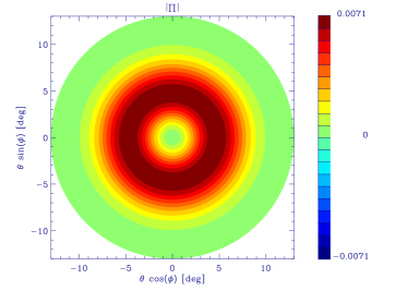
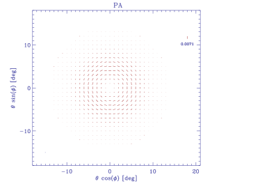
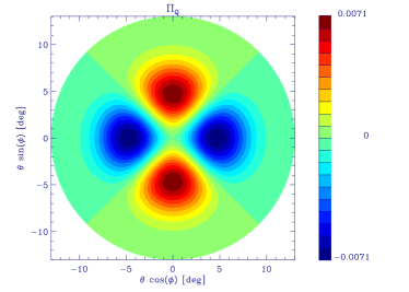
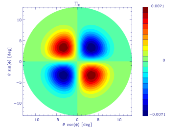
Figure 2: Instrumental polarization beams normalized to the co-polar maximum for the 90 GHz feed horn of the SPOrt experiment. The $|\Pi|$ map (top left) shows the axial symmetry of the beam, while the polarization angle map (top right: the vector length is proportional to the intensity) presents a radial pattern. In the case of SPOrt the polarization angles are tangential to the radial direction. The instrumental polarization beams $\Pi_{Q}$ (bottom left) and $\Pi_{U}$ (bottom right) have quadrilobe patterns that are symmetric with respect to the main axes; the change of sign from quadrant to quadrant makes the instrumental contamination in both $Q$ and $U$ only sensitive to the anisotropy pattern of the unpolarized radiation (see text for details).

3 Axisymmetric Case

Axial symmetry is an important special case representing several common optics solutions. Circular dual–polarization feed horns and on–axis mirror configurations like Cassegrain are some examples. The axial symmetry leads to some simplifications in the instrumental polarization equations with interesting effects on the $E$ and $B$-mode of the spurious polarization. In details, by considering the symmetric property of the radiation aperture, one co-polar pattern $g$ and one cross-polar $\chi$ are needed and the following relations hold (Rahmat-Samii 1993)

$$g_{x}(\theta,\,\phi) = g(\theta,\,\phi)$$

$$g_{y}(\theta,\,\phi) = g(\theta,\,\phi-\pi/2)$$

$$\chi_{x}(\theta,\,\phi) = \chi(\theta,\,\phi)$$

$$\chi_{y}(\theta,\,\phi) = -\chi(\theta,\,\phi-\pi/2)$$ (23)

together with the periodic and parity properties

$$g(\theta,\,\phi) = g(\theta,\,\phi+\pi)$$

$$g(\theta,\,\phi) = g(\theta,\,-\phi)$$

$$\chi(\theta,\,\phi) = \chi(\theta,\,\phi+\pi)$$

$$\chi(\theta,\,\phi) = -\chi(\theta,\,-\phi)$$ (24)

where $\theta$ is the angular distance from the axis and $\phi$ the azimuthal angle with respect to the instrument Cartesian reference frame centred on the main axis.

Considering these properties, equation (18) writes

$$Q_{\rm sp}+j\,\,U_{\rm sp} = {1\over 4\pi}\int_{0}^{\pi}\sin\theta\,d\theta\int_{0}^{\pi\over 2}d\phi\cdot$$ (25)

$$\left[T_{b}(\theta,\phi)-T_{b}(\theta,\phi+{\pi\over 2})\;+\right.$$

$$\left.T_{b}(\theta,\phi+\pi)-T_{b}(\theta,\phi+{3\over 2}\pi)\right]\cdot$$

$$\left[\Pi_{Q}(\theta,\phi)+j\,\Pi_{U}(\theta,\phi)\right]$$

where the integration is only performed over the first quadrant. The contribution of a constant $T_{b}$ term is null and the instrumental polarization in both $Q$ and $U$ only depends on the anisotropy of the unpolarized emission. This result extends equation (18) in Carretti et al. (2001) to $Q$.

Further properties of the axisymmetric case lead to a better understanding of the nature of this contamination and the instrumental polarization beam $\Pi=\Pi_{Q}+j\Pi_{U}$. In fact, $g$ and $\chi$ have the simple expressions

$$g(\theta,\,\phi) = g(\theta,\,\phi=0)\,\cos^{2}(\phi)+g(\theta,\,\phi={\pi\over 2})\,\sin^{2}(\phi)$$ (26)

$$= g_{0}(\theta)\,\cos^{2}(\phi)+g_{\pi/2}(\theta)\,\sin^{2}(\phi)$$

$$\chi(\theta,\,\phi) = {g_{0}(\theta)-g_{\pi/2}(\theta)\over 2}\sin(2\phi)$$ (27)

so that the instrumental polarization beams of $Q$ and $U$ result in

$$\Pi_{Q}(\theta,\,\phi) = {|g_{0}(\theta)|^{2}-|g_{\pi/2}(\theta)|^{2}\over 2}\;\cos(2\phi)$$ (28)

$$\Pi_{U}(\theta,\,\phi) = {|g_{0}(\theta)|^{2}-|g_{\pi/2}(\theta)|^{2}\over 2}\;\sin(2\phi)$$ (29)

and the contamination equation in

$$Q_{\rm sp}+j\,\,U_{\rm sp}={1\over 4\pi}\int_{\Omega}T_{b}(\theta,\phi)\ {|g_{0}|^{2}-|g_{\pi/2}|^{2}\over 2}\,e^{j2\phi}\,d\Omega.$$ (30)

The most relevant property of the instrumental polarization beam

$$\Pi=\Pi_{Q}+j\Pi_{U}={|g_{0}(\theta)|^{2}-|g_{\pi/2}(\theta)|^{2}\over 2}\,e^{j\,2\phi}$$ (31)

is the axial symmetry, with intensity only depending on the angular distance $\theta$ from the axis

$$|\Pi|=\left|{|g_{0}(\theta)|^{2}-|g_{\pi/2}(\theta)|^{2}\over 2}\right|$$ (32)

and polarization angle with radial pattern with respect to the beam axis

$$\alpha = 0.5\arctan\;{U_{\rm sp}\over Q_{\rm sp}}$$ (35)

$$= \left\{\begin{array}[]{ll}\phi&{\rm for\,|g_{0}|^{2}>|g_{\pi/2}|^{2}}\\ \phi+90^{\circ}&{\rm otherwise}.\\ \end{array}\right.$$

The angle $\alpha$ is directed either along the radial or the tangential direction depending on $|g_{0}|^{2}$ being larger or smaller than $|g_{\pi/2}|^{2}$. Moreover, the instrumental polarization is given by the difference between the co-polar cuts along the two main axes and it is thus related to asymmetries like differences in the FWHMs along the two axes.

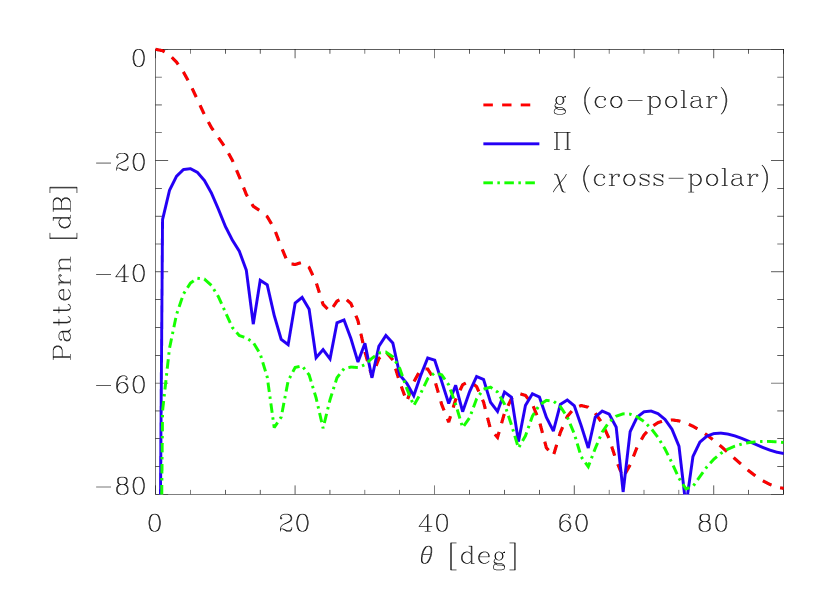
Figure 3: Amplitude of the instrumental polarization pattern $\Pi$ for the 90 GHz feed horn of the SPOrt experiment along a radial cut. The pattern is normalized to the maximum of the main beam. The co-polar and the cross-polar beams along the 45^∘ cut are also shown for comparison.

As an example, Figure 2 shows the case of the 90 GHz horn of SPOrt (Carretti et al. 2003). SPOrt is an experiment devoted to measure the Cosmic Microwave Background Polarization on large angular scales. It uses very simple antennae like circular feed horns with FWHM = $7^{\circ}$ resolution, intrisically axisymmetric. The axial symmetry of the instrumental polarized beam and the radial pattern of the polarization angles are clearly visible in the $|\Pi|$ and polarization angle maps. The $Q$ and $U$ responses present quadrilobe patterns and the change of sign with the quadrants makes the contamination in both $Q$ and $U$ only sensitive to the anisotropy of the unpolarized radiation (equation (25)). It is to be noted that $Q$ has the quadrilobe pattern along the main axes, while $U$ along the $45^{\circ}$ directions.

Figure 3 shows the section of the quantity $|\Pi|$ along one radial cut normalized to the co-polar beam maximum and provides the polarized contamination level as a function of the axial distance. The maximum is at about FWHM/2 from the antenna axis and the area where its action is effective has a diameter of about $2\times{\rm FWHM}$.

Finally, the representation in terms of amplitude and polarization angles of the contamination yields that the contaminations in both $Q$ and $U$ have the same nature and are simply the two components of a unique 2-D quantity.

4 Effects on $E$ and $B$-mode Power Spectra for the Axisymmetric Case

The $\Pi$ pattern is the response of the system to an unpolarized point source, the contamination being given by its convolution with $T_{b}$. In the axisymmetric case, $\Pi$ is axisymmetric in itself with polarization angle either parallel or perpendicular to the radial direction, suggesting that a pure $E$-mode is present with no contribution to $B$. To investigate the polarization power spectra of $\Pi$ we consider the simple case of an antenna pointing to the North Pole.

To compute the $E$- and $B$-mode spectra we have to write the $\Pi$ pattern in the polar basis where the spherical harmonics are referred to. The transformation is performed by parallel transporting the polarization vector along the great circle through the poles (Ludwig 1973)

$$\Pi^{\rm st}_{Q}+j\Pi^{\rm st}_{U}=(\Pi_{Q}+j\Pi_{U})\,e^{-j2\phi}.$$ (36)

The field $\Pi$ in the standard reference frame results thus in a $Q$ component depending only on $\theta$ and a null $U$ term

$$\Pi^{\rm st}_{Q} = \Pi_{Q}(\theta,0)={|g_{0}(\theta)|^{2}-|g_{\pi/2}(\theta)|^{2}\over 2},$$

$$\Pi^{\rm st}_{U} = 0.$$ (37)

From Zaldarriaga & Seljak (1997), for a field depending just on $\theta$ the only non-null 2-spin harmonic coefficients are $a_{\pm 2,\ell 0}$, which, in case of $U=0$, are real. Considering the relation $a_{2,\ell m}=a_{-2,\ell-m}^{*}$, the field $\Pi$ has $a_{2,\ell m}=a_{-2,\ell m}$ leading to the $E-$ and $B$–mode $\Pi$ coefficients

$$a_{E,\ell m}^{\Pi} = -a_{2,\ell 0}^{\Pi}\,\delta_{m\,0}$$

$$a_{B,\ell m}^{\Pi} = 0$$ (38)

and confirming that $\Pi$ has no $B$-mode in the axisymmetric case. Finally, the power spectra are

$$C_{E\ell}^{\Pi} = {1\over 2\ell+1}|a_{2,\ell 0}^{\Pi}|^{2},$$

$$C_{B\ell}^{\Pi} = 0.$$ (39)

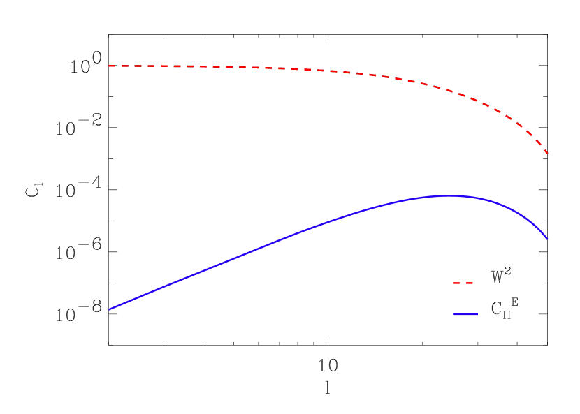
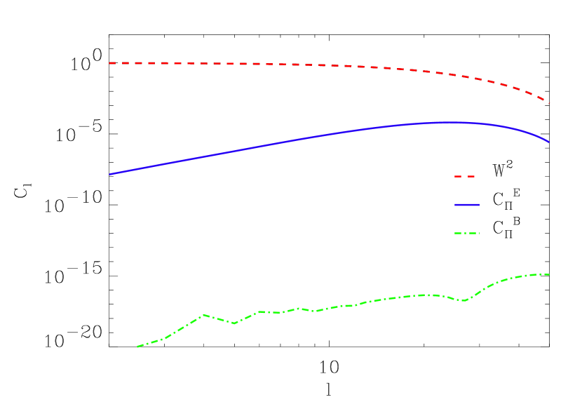
Figure 4: Top: $E$-mode power spectrum $C_{E}^{\Pi}$ of the instrumental polarization beam $\Pi$ for the SPOrt 90 GHz horn normalized to the spectrum of the window function $W_{\ell}^{2}$. The $E$-mode peaks nearly at the multipole typical of the FWHM ($\ell\sim 25$) leaving the larger scales significantly cleaner. Note that at $\ell=2$ the $E$ spectrum is about 4 orders of magnitude lower than at the peak and 8 orders of magnitude lower than the window function of the main beam. Bottom: the same plot with a larger range so to include the $B$-mode as well. Its level is much lower than the $E$ one and its presence is likely due to numerical errors. In any case, it is 12-13 orders of magnitude lower than the $E$-mode.

Figure 4 shows the spectra computed for the case of SPOrt horns. Beyond the very low level of the computed $B$-mode (non-zero value is likely due to numerical errors) an important property of the $E$-mode appears: its spectrum peaks at high $\ell$, approximately on the FWHM scale, and rapidly decreases at smaller $\ell$ leaving the largest scales significantly cleaner. This is a very important feature for instruments looking for CMBP on large scales, the relevant information being at $\ell<10$ (e.g. see Zaldarriaga, Spergel & Seljak 1997).

Besides the properties of $\Pi$, to understand the impact of instrumental polarization on CMBP experiments we have to evaluate the instrumental polarization map generated by a diffuse unpolarized emission.

In general, given a temperature map, equation (LABEL:tspSteq) states that the contamination field in not uniquely defined, depending on the rotation of the instrument with respect to the standard frame and, thus, on the scanning strategy.

This ambiguity is lost in the axisymmetric case, for which equation (31) holds and equation (LABEL:tspSteq) writes

$$Q_{\rm st}+jU_{\rm st} = {1\over 4\pi}\int_{\Omega}\left[R_{\bf{\hat{y}}}(\theta)R_{\bf{\hat{z}}}(\phi)T_{b}\right](\theta^{\prime\prime},\phi^{\prime\prime})$$

$$\Pi(\theta^{\prime\prime},0)\,e^{j2\phi^{\prime\prime}}\,d\Omega^{\prime\prime},$$

which is totally independent of the instrument rotation $\psi$ and corresponds to the contamination for an antenna aligned with the standard frame ($\psi=0$). Axisymmetric antennae have thus the interesting feature of generating instrumental polarization maps that are independent of the scanning strategy.

Figure 5: The position of $\bf{\hat{n}}=(\theta,\phi)$ with respect to $\bf{\hat{n}^{\prime}}=(\theta^{\prime},\phi^{\prime})$ is defined by three angles: $\beta$, the angular separation between the two versors; $\alpha$, the angle to take $\bf{\hat{e}}_{\theta}({\bf{\hat{n}}})$ in right-handed sense onto the great circle connecting $\bf{\hat{n}}$ and $\bf{\hat{n}^{\prime}}$; $\gamma$, the same as $\alpha$ but referred to $\bf{\hat{e}}_{\theta}({\bf{\hat{n}^{\prime}}})$.

From equation (31) and considering $\psi=0$, the contamination equation (LABEL:tspeq) writes

$$\left(Q_{\rm sp}+jU_{\rm sp}\right)({\bf{\hat{n}}})={1\over 4\pi}\int_{\Omega}T_{b}({\bf{\hat{n}^{\prime}}})\Pi(\beta,0)e^{j2\alpha}\,d\Omega^{\prime}\\$$

with $\beta$ the angle between the directions ${\bf{\hat{n}}}=(\theta,\phi)$ and ${\bf{\hat{n}^{\prime}}}=(\theta^{\prime},\phi^{\prime})$ and $\alpha$ the angle to rotate in the right-handed sense the versor ${\bf{\hat{e}}_{\theta}}({\bf{\hat{n}}})$ onto the great circle connecting ${\bf{\hat{n}}}$ and ${\bf{\hat{n}^{\prime}}}$ (see Figure 5).

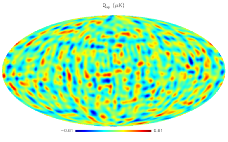
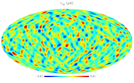
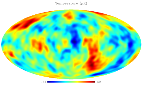
Figure 6: Contamination maps for $Q$(top) and $U$(mid) generated by the convolution between the $\Pi$ beam of the SPOrt horn and the Temperature map of a $\Lambda$CDM model (concordance model as from WMAP first year results). The Temperature map, smeared by the FWHM $\sim 7^{\circ}$ beam, is also shown (bottom).

Making use of the relation (Ng & Liu 1999)

$$Y_{s,\ell m}(\theta,\phi)=\sqrt{4\pi\over 2\ell+1}\sum_{m^{\prime}}Y_{s,\ell m^{\prime}}(\beta,\gamma)Y_{-m^{\prime},\ell m}(\theta^{\prime},\phi^{\prime})\,e^{js\alpha}$$

with $\gamma$ equivalent to $\alpha$ but for the direction ${\bf{\hat{n}^{\prime}}}$, the $a_{2,\ell m}^{T\otimes\Pi}$ coefficient of the contamination map results in

$$a_{2,\ell m}^{T\otimes\Pi} = \int d\Omega\,(Q_{\rm sp}+jU_{\rm sp})({\bf{\hat{n}}})\;Y_{2,\ell m}^{*}({\bf{\hat{n}}})$$

$$= {1\over\sqrt{4\pi\,\left(2\ell+1\right)}}\sum_{m^{\prime}}\int d\Omega^{\prime}\,T_{b}({\bf{\hat{n}^{\prime}}})Y_{-m^{\prime},\ell m}^{*}({\bf{\hat{n}^{\prime}}})\cdot$$

$$\int d\Omega_{\beta\gamma}\,Y_{2,\ell m^{\prime}}^{*}(\beta,\gamma)\Pi(\beta,0)$$

$$= {1\over\sqrt{4\pi\,\left(2\ell+1\right)}}\sum_{m^{\prime}}\int d\Omega^{\prime}\,T_{b}({\bf{\hat{n}^{\prime}}})Y_{-m^{\prime},\ell m}^{*}({\bf{\hat{n}^{\prime}}})\;a_{2,\ell m^{\prime}}^{\Pi}$$

where $d\Omega_{\beta\gamma}$ denotes the integration on the sphere centred on ${\bf{\hat{n}^{\prime}}}$. Since the last integral is the Since $a_{2,\ell m}^{\Pi}=a_{2,\ell 0}^{\Pi}\delta_{m0}$, it is straighforward

$$a_{2,\ell m}^{T\otimes\Pi} = {a_{2,\ell 0}^{\Pi}\over\sqrt{4\pi\,\left(2\ell+1\right)}}\int d\Omega^{\prime}\,T_{b}({\bf{\hat{n}^{\prime}}})Y_{\ell m}^{*}({\bf{\hat{n}^{\prime}}})$$ (43)

$$= {1\over\sqrt{4\pi\,\left(2\ell+1\right)}}\,\,{a_{2,\ell 0}^{\Pi}\,a_{\ell m}^{T}}.$$

Similarly,

$$a_{-2,\ell m}^{T\otimes\Pi} = {1\over\sqrt{4\pi\,\left(2\ell+1\right)}}\,\,{a_{-2,\ell 0}^{\Pi}\,a_{\ell m}^{T}},$$ (44)

leading to the power spectra of the contamination map

$$C_{E\ell}^{T\otimes\Pi} = {1\over 4\pi}\,C_{E\ell}^{\Pi}\,C_{T\ell},$$

$$C_{B\ell}^{T\otimes\Pi} = 0.$$ (45)

Thus, there is no $B$-mode component in the contamination map, and the $E$ power spectrum is the product between the spectra of the Temperature map $C_{T\ell}$ and the beam $\Pi$, making valid a sort of convolution theorem. Note that this result can be applied to all antenna systems with axisymmetric $\Pi$ pattern, even if, in general, this cannot be stated for off-axis optics.

To evaluate the effects of an axisymmetric optics on a CMBP experiment we take the example of the SPOrt instrument. The contamination maps $Q_{\rm sp}$ and $U_{\rm sp}$ are computed assuming a CMB anisotropy map compatible with the concordance model of the WMAP first-year data (Bennett et al. 2003, Spergel et al. 2003). We convolve the CMB temperature map with the SPOrt $\Pi$ beam considering the instrument aligned to the standard frame. The result is shown in Figure 6. A typical $E$-mode pattern is visible, with leading structures along parallels and meridians for $Q$ and along 45^∘–135^∘ directions for $U$.

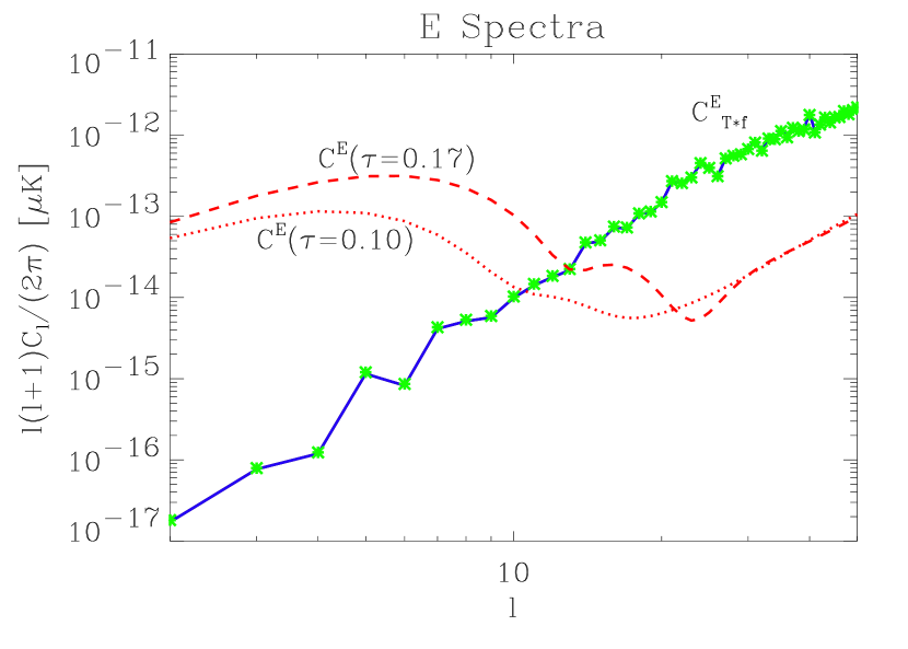
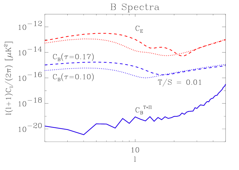
Figure 7: Top: $E$-mode power spectrum $C_{E}^{T\otimes\Pi}$ of the contamination maps of Figure 6 (solid) together with the product $C_{T}C_{E}^{\Pi}/4\pi$ between the spectra of the input temperature map and the instrumental beam $\Pi$ (stars). The spectra are corrected for the window function $W^{2}_{\ell}$ to account for the smearing effects of the main beam. For comparison, the CMBP $E$-mode spectrum for the WMAP best-fit model with optical depth $\tau=0.17$ is reported (dashed). A model with a smaller $\tau=0.10$ is also shown (dotted). Bottom: the same but for $B$. The spectrum of the contamination map $C_{B}^{T\otimes\Pi}$ (solid) is likely due to numerical noise. The expected CMBP spectra for two models with tensor-to-scalar ratio $T/S=0.01$ are several orders of magnitude above this level. The corresponding $E$ spectra are also shown.

The power spectra are shown in Figure 7. Here the spectra are corrected for the window function of the main beam $W^{2}_{\ell}$ to account for its smearing effects on $E$ and $B$ spectra (Zaldarriaga & Seljak 1997). As expected, the $B$-mode of the contamination map is at a very low level, likely due to numerical precision, and, in any case, is negligible when compared to the faint level of the cosmological signal (here we use a model with tensor-to-scalar ratio $T/S=0.01$).

The most important contamination in the $E$-mode is on FWHM scales and it rapidly decreases on larger ones, as expected from the $E$ spectrum of the SPOrt $\Pi$ pattern. Moreover, it is well fitted by the product between $C_{T}$ and $C_{E}^{\Pi}$. Figure 7 shows its comparison with the expected CMBP signal. At the large scale peak of CMBP ($\ell<10$), the instrumental polarization is nearly two orders of magnitude below the spectrum of the signal. This occurs not only for the best fit WMAP model ($\tau=0.17$), but also for a less reionized Universe ($\tau=0.10$). As a result, the SPOrt experiment does not look contaminated at significant level on the most relevant angular scales and no data cleaning seems to be needed. In any case, should an experiment suffer from a relevant leakage, it would be possible to subtract the spurious contribution estimated from both the Temperature Map and the $\Pi$ pattern. Equation (45) together with the variance equations for the Temperature spectra (Zaldarriaga & Seljak 1997) provides a way to estimate the residual noise after the subtraction: in the case of well known $\Pi$ pattern (negligible error) and Temperature map with uniform white noise, it results in

$$\sigma_{C_{E}}(\ell)={1\over 4\pi}\,\sqrt{2\over 2\ell+1}\,{C_{E\ell}^{\Pi}\over W^{2}_{\ell}}\,\,{\omega^{-1}_{T}\over W^{2}_{T\ell}}$$ (46)

with $W^{2}_{T\ell}$ the window function of the Temperature map and $\omega^{-1}_{T}=4\pi\sigma^{2}_{T,{\rm px}}/N_{\rm px}$, where $\sigma_{T,{\rm px}}$ is the pixel noise and $N_{\rm px}$ the number of pixels in the map. Finally, the window function of the main beam $W^{2}_{\ell}$ accounts for smearing effects on $E$.

5 Conclusions

We have derived the equations to compute the instrumental polarization introduced by the antenna. The contamination in both $Q$ and $U$ is the convolution of the unpolarized field of the incoming radiation with an instrumental polarization beam $\Pi=\Pi_{Q}+j\,\Pi_{U}$, which is a function of the co- and cross-polar patterns of the antenna. This result is general and independent of the technique adopted to measure $Q$ and $U$. In particular, it is valid for instruments either correlating the two polarizations (either circular or linear) or differentiating the two linear polarizations.

The special case of axisymmetric systems (like circular dual-polarization feed horns and on-axis mirrors) presents special features:

• The instrumental polarization pattern $\Pi$ is axisymmetric in itself with intensity only depending on the radial distance $\theta$ from the main axis;

• Polarization angles have a radial pattern and are either along or perpendicular to the radial direction;

• Both the instrumental beams $\Pi_{Q}$ and $\Pi_{U}$ of $Q$ and $U$ change sign from quadrant to quadrant, which makes the contamination only dependent on the anisotropy of the radiation;

• The contamination in the maps in the standard frame is independent of the instrument frame rotation and, in turn, of the scanning strategy of the experiment.

These features result in the relevant property that the $\Pi$ pattern has no $B$-mode component, leaving the $B$-mode of the sky signal uncontaminated.

This absence of leakage into the $B$-mode is an important result and makes axisymmetric systems suitable solutions for the detection of this faint signal. In general, off-axis solutions do not satisfy the axisymmetric condition and an analysis has to be performed for each case to evaluate the amount of instrumental polarization in $B$.

A further relevant result is that the spectrum of the $E$ component of the instrumental polarization is the product between the spectra of the unpolarized emission map and the instrumental polarization pattern. It peaks on FWHM scales, leaving significantly cleaner the larger ones. This represents an important result for CMBP experiments searching for signal on large scales, where the very new information provided by CMBP reside. As an example, the contamination generated in the SPOrt horns at $\ell=2$ is four orders of magnitude lower than at $\ell=25$ (FWHM $\sim 7^{\circ}$). Moreover, at $\ell<10$, where the CMBP has the large scale peak, the instrumental contribution of the SPOrt antennae is two orders of magnitude lower than the expected sky signal, probably making not necessary any correction for this systematic effect.

Experiments on small angular scales are in a different situation. They look for CMBP features close to the FWHM scale (the CMBP spectrum has several Doppler peaks in the 5–30 arcmin range) where the $E$-mode of the $\Pi$ pattern peaks. Moreover, the Doppler-peak pattern of the Temperature will be reproduced in some way in the spectrum of the contamination, leading to the possibility to confuse the peak pattern of the CMBP $E$-mode. A careful analysis of the instrumental polarization generated by the antenna system is thus mandatory for these experiments.

- (1) Bennett C.L., et al., 2003, submitted to ApJ, astro-ph//0302207
- (2) Berkhuijsen E.M., 1975, A&A, 40, 311
- (3) Carretti E., Tascone R., Cortiglioni S., Monari J., Orsini M., 2001, New Astron., 6, 173
- (4) Carretti E., et al., 2003, Polarimetry in Astronomy, Ed. S. Fineschi, SPIE Proc., 4843, 305
- (5) Challinor A., Fosalba P., Mortlock D., Ashdown M., Wandelt B., G rski K., 2000, Phys. Rev. D, 62, id. 123002
- (6) Franco G., Fosalba P., Tauber J. A., 2003, A&A, 405, 349
- (7) Kamionkowski M., Kosowsky A., 1998, Phys. Rev. D, 57, 685
- (8) Kaplan J., Delabrouille J, 2002, Astrophysical Polarized Backgrounds, Eds. S. Cecchini, S. Cortiglioni, R. Sault & C. Sbarra, AIP Conf. Proc., 609, 209
- (9) Kogut A., et al., 2003, submitted to ApJ, astro-ph//0302213
- (10) Kovac J.M., Leitch E.M., Pryke C., Carlstrom J.E., Halverson N.W., Holzapfel W.L., 2002, Nature, 420, 772
- (11) Kraus J.D., 1986, Radio Astronomy, Ed. Cygnus-Quasar Books, Ohio
- (12) Leahy J.P., Yurchenko V., Hastie M.A., Bersanelli M., Mandolesi N., 2002, Astrophysical Polarized Backgrounds, Eds. S. Cecchini, S. Cortiglioni, R. Sault & C. Sbarra, AIP Conf. Proc., 609, 215
- (13) Ludwig A.C., 1973, IEEE Trans. Antennas Propag. AP-21, 116
- (14) Ng K.-W., Liu G.-C., 1999, Int. J. Mod. Phys. D, 8, 61
- (15) Rahmat-Samii Y., 1993, Antenna handbook Vol. II, Chapter 15, Eds. Y.T. Lo & S.W. Lee, Van Nostrand Reinold, New York
- (16) Revenu B., Kim A., Ansari R., Couchot F., Delabrouille J., Kaplan J., 2000, A&AS, 142, 499
- (17) Sbarra C., Carretti E., Cortiglioni S., Zannoni M., Fabbri R., Macculi C., Tucci M., 2003, A&A, 401, 1215
- (18) Spergel D.N., et al., 2003, submitted to ApJ, astro-ph/0302209
- (19) Zaldarriaga M., Seljak U., 1997, Phys. Rev. D, 55, 1830
- (20) Zaldarriaga M., Spergel D.N., Seljak U., 1997, ApJ, 488, 1