Hydrodynamic Simulations of Tilted Thick-Disk Accretion onto a Kerr Black Hole

Abstract

We present results from fully general relativistic three-dimensional numerical studies of thick-disk accretion onto a rapidly-rotating (Kerr) black hole with a spin axis that is tilted (not aligned) with the angular momentum vector of the disk. We initialize the problem with the solution for an aligned, constant angular momentum, accreting thick disk, which is then allowed to respond to the Lense-Thirring precession of the tilted black hole. The precession causes the disk to warp, beginning at the inner edge and moving out on roughly the Lense-Thirring precession timescale. The propagation of the warp stops at a radius in the disk at which other dynamical timescales, primarily the azimuthal sound-crossing time, become shorter than the precession time. At this point, the warp effectively freezes into the disk and the evolution becomes quasi-static, except in cases where the sound-crossing time in the bulk of the disk is shorter than the local precession timescale. We see evidence that such disks undergo near solid-body precession after the initial warping has frozen in. Simultaneous to the warping of the disk, there is also a tendency for the midplane to align with the symmetry plane of the black hole due to the preferential accretion of the most tilted disk gas. This alignment is not as pronounced, however, as it would be if more efficient angular momentum transport (e.g. from viscosity or magneto-rotational instability) were considered.

1 Introduction

Quasars, active galactic nuclei (AGN), X-ray binaries, core-collapse supernovas, and gamma-ray bursts (GRBs) are among the most luminous objects in the universe and are therefore of considerable observational interest. They are also all likely to contain a central, strongly gravitating, compact object and be powered by some form of accretion. They are therefore also of considerable theoretical interest. However, the nonlinear, time-dependent, multi-dimensional nature of the physical laws governing these objects makes a study of them from first principles difficult. While such studies can provide critical insight, there is strong motivation to apply a numerical approach.

Many numerical simulations have been carried out over the past three decades studying the time-dependent evolution of accretion flows around black holes in the hydrodynamic (e.g. Wilson, 1972; Hawley et al., 1984; Hawley, 1991) and MHD (Koide et al., 1999; Gammie et al., 2003; De Villiers & Hawley, 2003) regimes. However, due to the complex nature of this problem, a variety of simplifying assumptions are normally implemented. A common simplification in much of the early work was to assume a non-rotating (Schwarzschild) black hole, often approximated using a pseudo-Newtonian (Paczynsky & Wiita, 1980) potential. A notable exception was the work of Wilson (1972), which considered the spherical infall of material with a non-zero specific angular momentum toward a Kerr black hole using the full metric, although restricted to two spatial dimensions. Although the assumption of a non-rotating black hole considerably simplifies the problem while still allowing useful insight, this does not appear to be well represented among observed black-hole systems (e.g. Elvis et al., 2002; Yu & Tremaine, 2002), nor does it agree with studies of black hole spin evolution (Gammie et al., 2004; Volonteri et al., 2004) which suggest that most black holes are likely to be spinning rapidly.

The spin of a black hole (often denoted by the specific angular momentum $a=J/M$) can have important consequences on the accretion rate and the geometry of the accretion flow. One obvious example is the dependence of $r_{ms}$, the radius of the marginally stable circular orbit, on the spin parameter [$r_{ms}=6r_{G}$ for $a=0$ (non-rotating black hole); $r_{ms}=r_{G}$ for $a=+M$ (maximal prograde rotation); $r_{ms}=9r_{G}$ for $a=-M$ (maximal retrograde rotation), where $r_{G}=GM/c^{2}$ is the gravitational radius (Bardeen et al., 1972)]. Another example is the reversal of flow direction in the vicinity of a rotating black hole for a retrograde accretion disk (see Figure 6 of De Villiers & Hawley, 2002).

Another common simplification in black hole accretion models has been the assumption that the midplane of the accretion flow is aligned with the symmetry plane of the black hole. This has historically been necessitated in numerical work by limitations in computing resources which have often limited simulations to two-dimensional axisymmetry. The justification for this treatment often relies on the Bardeen-Petterson effect (Bardeen & Petterson, 1975) through which a spinning black hole may align the inner region of the accretion flow with the symmetry plane of the black hole. However, now that computational resources are available to perform three-dimensional simulations of black-hole accretion, there are many compelling reasons to revisit the question of black-hole - disk alignment. First, the formation avenues for many black-hole - disk systems favor, or at least allow for, an initially tilted configuration (see Fragile et al. (2001) for a review of the arguments). Second, although the Bardeen-Petterson effect may align the inner disk, this alignment may not extend nearly as far out as was originally expected [$15-30r_{G}$ (Nelson & Papaloizou, 2000) rather than $100-1000r_{G}$]. Many numerical simulations extend to larger radii than this and, therefore, may not be justified in assuming that the midplane of the disk is aligned with the symmetry plane of the black hole. Finally, although there is a residual torque between the tilted outer disk and black hole which will eventually completely align the system (Rees, 1978; Scheuer & Feiler, 1996; Natarajan & Pringle, 1998), this happens over such a long timescale that these systems remain tilted for most of their observational lifetimes.

If an accretion disk is misaligned or tilted, it will be subject to differential Lense-Thirring precession. This is ultimately what gives rise to the Bardeen-Petterson effect. For an ideal test particle in a slightly tilted orbit at a radius $r$ around a black hole of mass $M$ and specific angular momentum $a$, gravitomagnetic torques cause the orbit to precess at a frequency $\Omega_{LT}=2aM/r^{3}$. Close to the black hole, this is comparable to the orbital frequency [$\Omega_{Kep}=(M/r^{3})^{1/2}$]. However, because of its strong radial dependence, Lense-Thirring precession becomes much weaker far from the hole. Nevertheless, since it has a cumulative effect, it can build up appreciably over a sufficiently large number of orbits. In an accretion disk, this cumulative build-up is limited by dynamic responses within the disk. For a steady-state disk, Lense-Thirring precession is expected to be important out to a unique, nearly constant transition radius (Bardeen & Petterson, 1975; Kumar & Pringle, 1985).

A comprehensive understanding of tilted accretion disks can be aided by the insights of direct numerical simulations. An important first step was taken by Nelson & Papaloizou (2000), who utilized a three-dimensional Newtonian SPH code to study tilted thin accretion disks subject to a post-Newtonian gravitomagnetic torque. In the current work we present results from three-dimensional, fully relativistic simulations of tilted black-hole accretion flows. A general relativistic treatment ensures that all important relativistic features, such as the cusp in the potential and the Einstein and Lense-Thirring precessions of the orbits, as well as any higher order couplings of these features, are treated properly. In this first study, we consider relatively simple, inviscid, thick accretion disks. These disks are well studied in the literature and provide a convenient starting point for our work. We should mention, however, that effective angular momentum transport (such as through viscous coupling as considered in Nelson & Papaloizou (2000)), would likely have a considerable impact on our results.

Unless otherwise stated, we use geometrized units ($G=c=1$) throughout this paper. Units of length are parameterized in terms of the gravitational radius of the black hole, $r_{G}=GM/c^{2}$. We also adopt the standard convention in which Greek (Latin) indices refer to 4(3)-space components.

2 Inviscid Accreting Thick Disks

Geometrically thick disks (often referred to as black hole tori or toroidal neutron stars) have been proposed to form through a number of scenarios, including the collapse of supermassive neutron stars (Vietri & Stella, 1998), the iron-core collapse of a massive stars (MacFadyen & Woosley, 1999), and the mergers of black hole - neutron star binaries (Lee & Kluźniak, 1999). They may also exist in the inner regions of more standard accretion flows. These disks are convenient to study numerically as they represent an equilibrium solution in the limit that self-gravity, radiation, and viscosity are negligible. However, they are subject to numerous instabilities: 1) the so-called “runaway instability” in tori with non-negligible mass and accretion (Font & Daigne, 2002); 2) the magneto-rotational instability (MRI, Balbus & Hawley, 1991); and 3) the Papaloizou-Pringle instability (PPI, Papaloizou & Pringle, 1984). In this work, we assume that the mass of the torus is negligible compared to the mass of the black hole, thus allowing us to neglect the runaway instability. This also allows us to ignore the self-gravity of the torus gas and treat the background metric as fixed. We also ignore magnetic fields in the current work, so the MRI is not applicable. Below we discuss how the PPI affects our work in more detail.

The analytic solution for the structure of a thick disk has been worked out for both non-rotating and rotating black holes in the limit of axisymmetry (Fishbone & Moncrief, 1976; Abramowicz et al., 1978). However, no such solution has been worked out for more general tilted flows. Furthermore, it is not clear that a steady-state solution would result. In light of the violent formation scenarios proposed above, however, it seems likely a newly formed torus will be highly disturbed and possibly have an orbital plane that is tilted with respect to the symmetry plane of the black hole. This, in fact, is part of the motivation for this numerical study. Nevertheless, we are left with a decision about how to initialize the problem. We choose to initialize all our disks with the analytic solution for an axisymmetric thick disk, which is subsequently allowed to respond to the Lense-Thirring precession of a tilted black hole.

For untilted accreting thick disks, the gas flows in an effective (gravitational plus centrifugal) potential. Since axisymmetric thick disks have been described in great detail elsewhere (e.g. Kozlowski et al., 1978), we present only a brief discussion here. Surfaces of constant pressure in the torus are determined from the relativistic analog of the Newtonian effective potential $\Phi$,

$$\Phi-\Phi_{in}=-\int^{P}_{0}\frac{\mathrm{d}P}{\rho h}~{},$$ (1)

where $P$ is the fluid pressure, $\rho$ is the density, $h$ is the relativistic enthalpy, and $\Phi_{in}$ is the potential at the boundary of the torus (where $P=0$). For constant angular momentum $l$, the form of the potential reduces to $\Phi=\ln(-u_{t})$, where $u_{t}$ is the specific binding energy. Provided $l>l_{ms}$, where $l_{ms}$ is the angular momentum of the marginally stable Keplerian orbit, the potential $\Phi(r,\theta)$ will have a saddle point $\Phi_{cusp}$ at $r=r_{cusp}$, $\theta=\pi/2$. We can define the parameter $\Delta\Phi=\Phi_{in}-\Phi_{cusp}$ as the potential barrier (energy gap) at the inner edge of the torus. If $\Delta\Phi<0$, the torus lies entirely within its Roche lobe. Such a configuration is marginally stable with respect to local axisymmetric perturbations and unstable to low-order non-axisymmetric PPI modes (Papaloizou & Pringle, 1984). If $\Delta\Phi>0$, the torus overflows its Roche lobe and accretion occurs through pressure-gradient forces across the cusp. This accretion occurs without dissipation of angular momentum; thus viscosity is not required for accretion. This accretion generally suppresses the growth of instabilities in the torus (Hawley, 1991). All of the simulations presented in this work begin with $\Delta\Phi>0$.

3 Hydrodynamic Equations in Kerr Geometry

In this work, we solve the system of equations for relativistic hydrodynamics in flux-conserving form (Anninos & Fragile, 2003)

$$\frac{\partial D}{\partial t}+\frac{\partial(DV^{i})}{\partial x^{i}} = 0,$$ (2)

$$\frac{\partial E}{\partial t}+\frac{\partial(EV^{i})}{\partial x^{i}}+P\frac{\partial W}{\partial t}+P\frac{\partial(WV^{i})}{\partial x^{i}} = 0$$ (3)

$$\frac{\partial S_{j}}{\partial t}+\frac{\partial(S_{j}V^{i})}{\partial x^{i}}-\frac{S^{\mu}S^{\nu}}{2S^{0}}\frac{\partial g_{\mu\nu}}{\partial x^{j}}+\sqrt{-g}\frac{\partial P}{\partial x^{j}} = 0,$$ (4)

where $g$ is the determinant of the 4-metric, $W=\sqrt{-g}u^{t}$ is the relativistic boost factor, $D=W\rho$ is the generalized fluid density, $P=(\Gamma-1)E/W$ is the fluid pressure, $V^{i}=u^{i}/u^{t}$ is the transport velocity, $S_{i}=W\rho hu_{i}$ is the covariant momentum density, and $E=We=W\rho\epsilon$ is the generalized internal energy density.

These equations are evolved in a “tilted” Kerr-Schild polar coordinate system $({t},{r},{\vartheta},{\varphi})$. This coordinate system is related to the usual (untilted) Kerr-Schild coordinates $({t},{r},{\theta},{\phi})$ through a simple rotation about the ${y}$-axis by an angle $\beta_{0}$, such that

$$\left(\begin{array}[]{c}\sin{{\vartheta}}\cos{{\varphi}}\\ \sin{{\vartheta}}\sin{{\varphi}}\\ \cos{{\vartheta}}\end{array}\right)=\left(\begin{array}[]{ccc}\cos{\beta_{0}}&0&-\sin{\beta_{0}}\\ 0&1&0\\ \sin{\beta_{0}}&0&\cos{\beta_{0}}\end{array}\right)\left(\begin{array}[]{c}\sin{{\theta}}\cos{{\phi}}\\ \sin{{\theta}}\sin{{\phi}}\\ \cos{{\theta}}\end{array}\right)~{}.$$ (5)

The Kerr line element in the tilted $({t},{r},{\vartheta},{\varphi})$ coordinate system is

$$\mathrm{d}s^{2} = -\left(1-\frac{2Mr}{\varrho^{2}}\right)\mathrm{d}t^{2}+\frac{4Mr}{\varrho^{2}}\mathrm{d}t\mathrm{d}r-\frac{4Mar\sin^{2}\theta}{\varrho^{2}}P_{1}\mathrm{d}t\mathrm{d}\vartheta$$ (6)

$$-\frac{4Mar\sin^{2}\theta}{\varrho^{2}}P_{2}\mathrm{d}t\mathrm{d}\varphi+\left(1+\frac{2Mr}{\varrho^{2}}\right)\mathrm{d}r^{2}$$

$$-2a\sin^{2}\theta\left(1-\frac{2Mr}{\varrho^{2}}\right)P_{1}\mathrm{d}r\mathrm{d}\vartheta$$

$$-2a\sin^{2}\theta\left(1-\frac{2Mr}{\varrho^{2}}\right)P_{2}\mathrm{d}r\mathrm{d}\varphi$$

$$+\left(\varrho^{2}T_{1}^{2}+AP_{1}^{2}\right)\mathrm{d}\vartheta^{2}+2\left(\varrho^{2}T_{1}T_{2}+AP_{1}P_{2}\right)\mathrm{d}\vartheta\mathrm{d}\varphi$$

$$+\left(\varrho^{2}T_{2}^{2}+AP_{2}^{2}\right)\mathrm{d}\varphi^{2}~{},$$

with

$$\varrho^{2} \equiv r^{2}+a^{2}\cos^{2}\theta$$

$$\Delta \equiv r^{2}-2Mr+a^{2}$$

$$A \equiv \frac{\left[\left(r^{2}+a^{2}\right)^{2}-\Delta a^{2}\sin^{2}\theta\right]\sin^{2}\theta}{\varrho^{2}}$$

$$T_{1} \equiv \frac{-1}{\sin\theta}\frac{\mathrm{d}(\cos\theta)}{\mathrm{d}\vartheta}$$

$$T_{2} \equiv \frac{-1}{\sin\theta}\frac{\mathrm{d}(\cos\theta)}{\mathrm{d}\varphi}$$

$$P_{1} \equiv \frac{1}{\cos\phi}\frac{\mathrm{d}(\sin\phi)}{\mathrm{d}\vartheta}$$

$$P_{2} \equiv \frac{1}{\cos\phi}\frac{\mathrm{d}(\sin\phi)}{\mathrm{d}\varphi}~{},$$ (7)

where $\sin\theta$, $\cos\theta$, $\sin\phi$, and $\cos\phi$ are given by equation 5. For a Schwarzschild ($a=0$) or an aligned Kerr black hole ($\beta_{0}=n\pi$, where $n=0,1,2,$…), the $({t},{r},{\vartheta},{\varphi})$ and $({t},{r},{\theta},{\phi})$ frames are equivalent.

The computational advantages of the “horizon-adapted” Kerr-Schild form of the Kerr metric are described in Papadopoulos & Font (1998) and Font et al. (1998). The primary advantage is that, unlike Boyer-Lindquist coordinates, there are no singularities in the metric terms at the event horizon. This is particularly important for numerical calculations as it allows one to place the grid boundaries inside the horizon, thus ensuring that they are causally disconnected from the rest of the flow.

4 Numerical Methods

Our main purpose in this work is to examine the structure of tilted accreting thick disks orbiting around a Kerr black hole. In practice, we actually initialize the disks aligned with the computational grid and tilt the black hole through a transformation of the metric. We have tested problems with the disk tilted relative to the grid and found similar results. We carry out these simulations using Cosmos, a massively parallel, multidimensional, radiation-chemo-magnetohydrodynamic code for both Newtonian and relativistic flows. The relativistic capabilities and tests of Cosmos are discussed in Anninos & Fragile (2003). The present work utilizes the zone-centered artificial viscosity hydrodynamics package in Cosmos.

The simulations are initialized with the analytic solution for an axisymmetric torus with constant specific angular momentum $l$ around a rotating black hole with spin $a$. For the initialization, we assume an isentropic equation of state $P=\kappa\rho^{\Gamma}$, although during the evolution the adiabatic form $P=(\Gamma-1)E/W$ is used to recover the pressure when solving equations (2) - (4). For all but one model, we set $\Gamma=4/3$ and $\kappa=1.06\times 10^{11}$ (in cgs units). The surface of the torus is defined by the effective potential at the boundary of the torus $\Phi_{in}$, although in practice the torus is cut off where the fluid density and pressure match the background values. All of our runs are initialized with a positive energy gap $\Delta\Phi=\Phi_{in}-\Phi_{cusp}>0$, where $\Phi_{cusp}$ is the saddle point in the potential at $r=r_{cusp}$, $\theta=\pi/2$. With this choice, a small fraction of the torus mass is initially out of equilibrium.

The simulations are carried out on a grid extending from $0.98r_{BH}\leq r\leq r_{max}$, $0\leq\vartheta\leq\pi$, and $0\leq\varphi<2\pi$, where $r_{BH}$ is the radius of the black hole horizon. We choose $r_{max}$ such that the disk is initially contained entirely within the computational domain. In order to increase the resolution in the inner region of the disk, we replace the radial coordinate ${r}$ with a logarithmic coordinate $\eta=1+\ln(r/r_{BH})$. In terms of this logarithmic coordinate, the grid extends from $0.98\leq\eta\leq\eta_{max}$, with a typical radial grid spacing of $0.2r_{G}$ near the horizon and $6r_{G}$ near the outer boundary. Zones are evenly spaced in both angular dimensions. The grid is normally resolved with $96\times 64\times 96$ zones along the dimensions $\eta$, $\vartheta$, $\varphi$. This resolution is sufficient to resolve key disk properties such as the PPI. To illustrate this point and demonstrate the ability of our code to reproduce other published work, we plot in Figure 1 the growth of the $m=1$ and $m=2$ PPI modes for a simulation comparable to Model A3p of De Villiers & Hawley (2002) using a $64\times 64\times 64$ grid. Our results are very similar to those of de Villiers & Hawley as seen by comparing to their Figure 7. Additional verification of our results is provided by comparing simulations at different grid resolutions in order to study the self-convergence of our solutions.

Figure 1: PPI mode growth for comparison with Model A3p of De Villiers & Hawley (2002).

In the “background” regions not determined by the initial torus solution, we initialize the gas following the spherical Bondi accretion solution. We fix the parameters of this solution such that the rest mass present in the background is negligible ($\lesssim 10^{-2}$) compared to the mass in the torus. Similarly, the mass accretion from the background is generally small ($\lesssim 10^{-3}$) compared to the mass accretion from the disk. The outer radial boundary is held fixed with the analytic Bondi solution for all evolved fields. The inner radial boundary uses simple flat (zero gradient) boundary conditions. Data are shared appropriately across angular boundaries.

After the torus and background are initialized, the black hole is tilted by an angle $\beta_{0}$ through a transformation of the metric. Each model is evolved to $t\gtrsim 10\tau_{orb}$, where $\tau_{orb}$ is the orbital period measured at the pressure (and density) maximum of the axisymmetric torus (denoted $r_{center}$). Most of the disks achieve a quasi-steady state [i.e. variations in measured disk properties, such as the twist and tilt, are small ($<10$%) over dynamical timescales] by the end of the simulations. The principle exceptions are disks that undergo near solid-body precession and disks that accrete a large percentage of their mass ($\gtrsim 50\%$) onto the black hole.

To describe our results more thoroughly, we track a number of quantities throughout the simulations, including the mass accretion rate, the PPI mode growth for the azimuthal wavenumbers $m=1$ and 2, and the precession angle (twist) and angle of inclination (tilt) of the disk. The mass accretion rate is defined as

$$\dot{M}(r)=\int^{2\pi}_{0}\int^{\pi}_{0}DV^{r}\mathrm{d}\vartheta\mathrm{d}\varphi~{}.$$ (8)

The accretion rates are converted to units with a polytropic constant $\kappa=1.5\times 10^{20}$ (cgs units) and mass $M=1M_{\odot}$, consistent with Igumenshchev & Beloborodov (1997). This value is then normalized by the Eddington accretion rate $\dot{M}_{Edd}=L_{Edd}/c^{2}\approx 1.4\times 10^{17}(M/M_{\odot})$ g s^-1. The conversion of $\dot{M}$ is accomplished through the relation

$$\left(\frac{\dot{M}}{\dot{M}_{Edd}}\right)_{new}=\frac{(M)_{new}}{(M)_{old}}\left(\frac{\kappa_{new}}{\kappa_{old}}\right)^{-1/(\Gamma-1)}\left(\frac{\dot{M}}{\dot{M}_{Edd}}\right)_{old}~{}.$$ (9)

Using this common scaling allows for easy comparison of our results. Nevertheless, we caution the reader against attaching any particular physical significance to these values since the mass accretion rates and densities in these simulations are essentially arbitrary.

The $m=1$ and 2 Fourier modes of the PPI are extracted by computing azimuthal density averages of the following form (De Villiers & Hawley, 2002)

$$\mathrm{Re}[k_{m}(r)]=\int_{0}^{2\pi}\rho(r,\pi/2,\varphi)\cos(m\varphi)d\varphi~{},$$ (10)

$$\mathrm{Im}[k_{m}(r)]=\int_{0}^{2\pi}\rho(r,\pi/2,\varphi)\sin(m\varphi)d\varphi~{}.$$ (11)

The power in mode $m$ is then

$$f_{m}=\frac{1}{r_{max}-r_{min}}\int_{r_{min}}^{r_{max}}\ln(\{\mathrm{Re}[k_{m}(r)]\}^{2}+\{\mathrm{Im}[k_{m}(r)]\}^{2})dr~{},$$ (12)

where $r_{min}$ and $r_{max}$ are the approximate inner and outer edges of the disk.

We define the precession angle (twist) as (Nelson & Papaloizou, 2000)

$$\gamma(r)=\arccos\left[\frac{\mathbf{J}_{BH}\times\mathbf{J}_{Disk}(r)}{|\mathbf{J}_{BH}\times\mathbf{J}_{Disk}(r)|}\cdot\hat{y}\right]~{},$$ (13)

where

$$\mathbf{J}_{BH}=\left(-aM\sin\beta_{0}\hat{x},0,aM\cos\beta_{0}\hat{z}\right)$$ (14)

is the angular momentum vector of the black hole and

$$\mathbf{J}_{Disk}(r)=\left[(J_{Disk})_{1}\hat{x},(J_{Disk})_{2}\hat{y},(J_{Disk})_{3}\hat{z}\right]$$ (15)

is the angular momentum vector of the disk in an asymptotically flat space, where

$$(J_{Disk})_{\rho}=\frac{\epsilon_{\mu\nu\sigma\rho}L^{\mu\nu}S^{\sigma}}{2\sqrt{-S^{\alpha}S_{\alpha}}}$$ (16)

and

$$L^{\mu\nu}=\int\left(x^{\mu}T^{\nu 0}-x^{\nu}T^{\mu 0}\right)\mathrm{d}^{3}x,$$ (17)

with $S^{\sigma}=\int T^{\sigma 0}\mathrm{d}^{3}x$, $T^{\mu\nu}=\rho hu^{\mu}u^{\nu}+Pg^{\mu\nu}$, and $\beta_{0}$ is the initial tilt between the angular momentum vectors of the black hole and the disk. The equations for $L^{\mu\nu}$ and $S^{\sigma}$ are integrated over concentric radial shells of the grid. The unit vector $\hat{y}$ points along the axis about which the black hole is initially tilted and $\hat{z}$ points along the initial symmetry axis of the disk. Thus, from Equation (13), $\gamma(r)=0$ throughout the disk at $t=0$. In order to capture twists larger than $180^{\circ}$, we also track the projection of $\mathbf{J}_{BH}\times\mathbf{J}_{Disk}(r)$ onto $\hat{x}$, allowing us to break the degeneracy in $\arccos$. We use the condition $\gamma=1$ to define a transition radius $r_{T}$ between an inner twisted disk (precession greater than 1 radian) and the outer undisturbed disk.

The angle of inclination (tilt) in the disk is defined as (Nelson & Papaloizou, 2000)

$$\beta(r)=\arccos\left[\frac{\mathbf{J}_{BH}\cdot\mathbf{J}_{Disk}(r)}{|\mathbf{J}_{BH}||\mathbf{J}_{Disk}(r)|}\right]~{}.$$ (18)

The models are set up such that, initially, $\beta(r)=\beta_{0}$ throughout the disk. For tilted disks ($\beta_{0}\neq 0$) such as the ones considered in this work, Lense-Thirring precession proceeds most rapidly closest to the black hole and gradually affects the disk further out as the simulations progress.

We expect differential Lense-Thirring precession to dominate whenever the precession timescale $\tau_{LT}=\Omega_{LT}^{-1}$ is shorter than local dynamical timescales in the disk (Bardeen & Petterson, 1975; Kumar & Pringle, 1985). We consider two possible limiting timescales: the mass accretion timescale $\tau_{acc}=(r-r_{BH})/\overline{V}^{r}$, where $\overline{V}^{r}$ is the average inflow velocity of the torus gas, and the azimuthal sound-crossing time defined as $\tau_{cs}=\pi r/c_{s}$, where $c_{s}$ is the local sound speed in the density midplane. In this work we determine the accretion timescale numerically from $\overline{V}^{r}=\dot{M}/\lambda$, where $\lambda(r)\equiv\int\int D\mathrm{d}\vartheta\mathrm{d}\varphi$. Initially the sound speed in the disk is given by $c_{s}^{2}=(\Gamma-1)(1-u_{t}/u_{t,in})$. During the evolution, the local sound speed is recovered from the fluid state through the relation $c_{s}^{2}=\Gamma(\Gamma-1)P/[(\Gamma-1)\rho+\Gamma P]$. Since the sound speed is defined in the proper frame of the fluid, it is not strictly accurate to compare $\tau_{cs}$ to quantities defined using the coordinate time (such as $\tau_{LT}$). However, the corrections are only of order $Mr/(r^{2}+a^{2})$ and should therefore be small ($\lesssim 20$%) for the radii of interest here.

5 Results

In this work we present results from eleven different models, varying the spin of the black hole, the angular momentum and tilt of the torus, the magnitude of the energy gap, the sound speed within the disk, and the size and resolution of the grid. The basic parameters for each model are listed in Table 1. Many of our parameters closely match those of Models II and III in Igumenshchev & Beloborodov (1997), thus providing us with an avenue to compare our results with other numerical simulations. However, we emphasize that there are a number of significant differences between their simulations and ours: all of the simulations reported here are performed in three dimensions and all but one are tilted; we use the Kerr-Schild form of the Kerr metric; we use a logarithmic radial coordinate for higher resolution near the black hole; and we choose a different inner surface potential $\Phi_{in}$. In the following sections we describe the results of each of our models in more detail.

Table 1: Tilted Thick-Disk Models

	Grid
Model	($N_{\eta}\times N_{\vartheta}\times N_{\varphi}$)	$a/M$	$l/M$	($t_{orb}/M$)	$\Delta\Phi$	$\beta_{0}$
t90	$96\times 64\times 96$	0.9	2.6088	46.1	0.03	0
t915XL	$24\times 24\times 24$	0.9	2.6088	46.1	0.03	15∘
t915L	$48\times 24\times 48$	0.9	2.6088	46.1	0.03	15∘
t915H	$96\times 64\times 96$	0.9	2.6088	46.1	0.03	15∘
t915H2	$96\times 64\times 96$	0.9	2.6088	46.1	0.04	15∘
t930L	$48\times 24\times 48$	0.9	2.6088	46.1	0.03	30∘
t930H	$96\times 64\times 96$	0.9	2.6088	46.1	0.03	30∘
t915$\Gamma$	$48\times 24\times 48$	0.9	2.6088	46.1	0.03	15∘
t915R	$96\times 64\times 96$	-0.9	4.4751	255.	0.0175	15∘
t515L	$48\times 24\times 48$	0.5	3.385	118.	0.004	15∘
t515H	$96\times 64\times 96$	0.5	3.385	118.	0.004	15∘

5.1 Model t90

This is the only model without an initial tilt between the symmetry plane of the black hole and the midplane of the torus. The black hole has a spin $a/M=0.9$ and radius $r_{BH}/r_{G}=1.44$; the torus has a specific angular momentum $l/M=2.6088$ and a density center at $r_{center}/r_{G}=3.45$. The cusp in the potential is located at $r_{cusp}/r_{G}=1.76$, $\theta=\pi/2$ with $\Phi_{cusp}=-0.04$. We choose an inner surface potential $\Phi_{in}=-0.01$ giving an energy gap $\Delta\Phi=0.03$. The outer boundary is set at $r_{max}/r_{G}=80$ and the simulation is evolved until $t=490M\approx 10\tau_{orb}$. This untilted simulation is included primarily to illustrate that our base model is not susceptible to the Papaloizou-Pringle instability, owing to the relatively large, positive energy gap at the cusp leading to a moderately high accretion rate that suppresses the growth of PPI (Hawley, 1991). In Figure 2a we show (a) the final distribution of torus gas density, (b) the time evolution of the mass accretion rate at the black hole horizon, and (c) the growth rates for the $m=1$ and $m=2$ PPI modes.

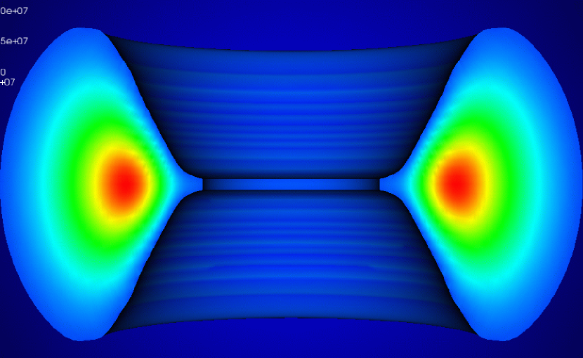
Figure 2a: Model t90. (a) Linear density plot at $t=490M\approx 10\tau_{orb}$. For rendering purposes, the surface of the torus is set at $\rho_{surf}\approx 0.1\rho_{max}$ and half the torus is cut away. To give a clearer view of the central region, the image is zoomed in to a small fraction of the total computational volume. The image is plotted in logarithmic coordinate space, where $x=\eta\sin\vartheta\cos\varphi$, $y=\eta\sin\vartheta\sin\varphi$, and $z=\eta\cos\vartheta$. The torus is only initialized in the region $r\geq r_{cusp}$. The black hole (not pictured) lies at the center of the image. (b) Mass accretion rate $\dot{M}$ at the black hole horizon in units of the Eddington mass accretion rate $\dot{M}_{Edd}$ (assuming $M_{BH}=1M_{\odot}$ and $\kappa=1.5\times 10^{20}$ in cgs units). (c) PPI mode growth.

Figure 2b:

Figure 2c:

The mass accretion rate (Figure 2ab) starts at a small value fixed by the background Bondi solution. Gas from the disk begins its infall from $r>r_{cusp}$ and so experiences a short delay before reaching the black hole horizon. After a short transition time ($\lesssim 3t_{orb}$), $\dot{M}$ asymptotes toward a stationary value. However, the initial adjustment of the disk generates an outgoing wave within the disk that is reflected at the outer disk edge. The arrival of this wave back at the inner edge of the disk causes the “bump” in the accretion rate at late time. A similar behavior is seen in many of our models. Although this feature shows up very clearly in the accretion rate, it does not appear to have a significant effect on any of the other disk properties we track. This is consistent with our findings throughout this study that the tilt and twist of these disks are not strongly responsive to the mass accretion rate. Furthermore, we note from our longer runs below (see Model t915L) that this feature does not recur at later times; after the wave reaches the inner edge of the disk, it passes through the cusp and black-hole horizon and is not reflected. It, therefore, has no further impact on the problem. Based upon this behavior, it appears that this feature is either not related to the axisymmetric oscillation modes studied in Zanotti et al. (2003) or that the large value of $\Delta\Phi$ (energy gap) prevents the oscillation mode from being sustained.

Although the PPI is seeded with small ($\lesssim 1$%) random fluctuations in the initial mass and internal energy densities, its growth is suppressed and the torus becomes essentially smooth and axisymmetric. This is consistent with the findings of De Villiers & Hawley (2002) that the PPI is suppressed whenever the accretion rate is high as in our models. In fact, this motivated our choice of parameters for these models, as we wanted to avoid the complication of PPI in this study.

5.2 Models t915XL, t915L, & t915H

These models begin from exactly the same initial conditions as Model t90 except that the black hole is tilted by an angle $\beta_{0}=15^{\circ}$. Thus, these disks are subject to Lense-Thirring precession. Model t915XL uses a resolution of $24\times 24\times 24$ zones and Model t915L uses a resolution of $48\times 24\times 48$; both are evolved until $t=1400M\approx 30\tau_{orb}$. Model t915H uses a resolution of $96\times 64\times 96$ and is evolved until $t=490M\approx 10\tau_{orb}$. Figure 3a shows (a) the final distribution of torus gas density for Model t915H, (b) the cumulative precession $\gamma$ and (c) tilt $\beta$ of the disk as a function of the logarithmic radial coordinate $\eta$, (d) the mass accretion rate $\dot{M}$ at the black hole horizon as a function of time, and (e) the time evolution of the transition radius $r_{T}$ defined as the radius where the twist equals 1 radian ($\gamma=1$). It is clear from Figures 3aa, 3ab, and 3ac that the disk is strongly twisted and warped at the end of the simulation. Nevertheless, the disk reaches a quasi-steady state before the simulations are stopped. This claim is supported by the following observations: 1) in Figure 3ab, the twist profile changes only slightly from $t=10\tau_{orb}$ to $t=30\tau_{orb}$; 2) in Figure 3ad, the mass accretion rate asymptotes toward a constant value; and 3) in Figure 3ae, the transition radius also asymptotes toward a constant value.

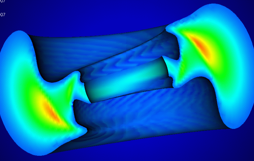
Figure 3a: Model t915L & t915H. (a) Linear density profile (similar to Figure 2aa) for Model t915H at $t=490M\approx 10\tau_{orb}$. The black hole spin axis is tilted $15^{\circ}$ to the left of the $z$-axis. (b) Cumulative precession angle $\gamma$ and (c) tilt $\beta$ in radians as functions of radius. Initially, $\gamma=0$ and $\beta=15^{\circ}\approx 0.26$ throughout the disks. (d) Mass accretion rate in units of the Eddington mass accretion rate. (e) Transition radius (symbols) as a function of time along with the Lense-Thirring precession timescale $\tau_{LT}$ (solid), azimuthal sound crossing time $\tau_{cs}$ (dashed), and accretion timescale $\tau_{acc}$ (dot-dashed). The thin vertical line marks the radius where $\tau_{LT}=\tau_{cs}$.

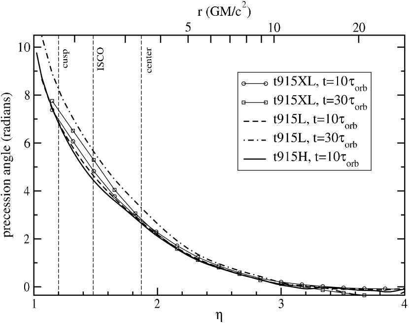
Figure 3b:

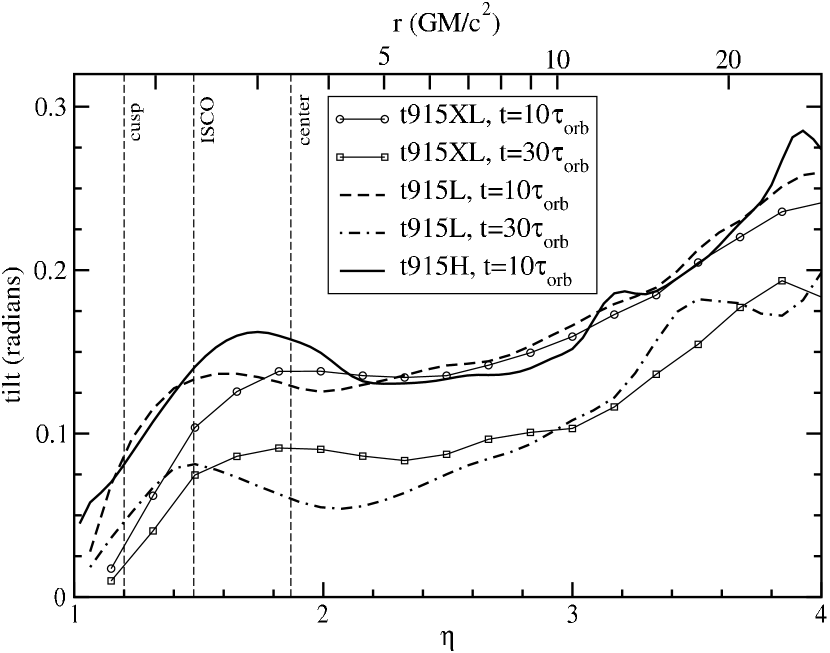
Figure 3c:

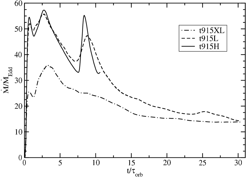
Figure 3d:

Figure 3e:

Although the transition radius in Figure 3ae starts out closely following the expected growth of Lense-Thirring precession for ideal test particles ($r_{T}\propto t^{1/3}$), it eventually approaches a limiting value of $r_{T}\lesssim 7r_{G}$. This is approximately coincident with the radius at which the local azimuthal sound-crossing time $\tau_{cs}$ (dashed line in Figure 3ae) becomes shorter than the Lense-Thirring precession timescale $\tau_{LT}$ (thick solid line). This finding appears consistent with the expectations of Nelson & Papaloizou (2000) that warps in thick disks are diffused by wave modes. As the disk is twisted up by Lense-Thirring precession, the twist is diffused away by dynamical responses in the disk. We note that the accretion timescale $\tau_{acc}$ (dot-dashed line) in these disks is significantly longer than the Lense-Thirring or sound-crossing timescales except in the outer regions ($r>15r_{G}$). As such, it does not appear to play a role in limiting the precession. Nevertheless, we point out that this tilted disk is subject to a higher accretion rate than the untilted model (compare Figures 3ad and 2ab). This is expected since more of the tilted torus begins the simulation out of equilibrium.

A curious feature seen in Figure 3ac and evident in nearly all of our models is the tendency for these disks to align toward the symmetry plane of the black hole despite the lack of viscous angular momentum transport. This alignment seems to be facilitated by the preferential accretion of highly tilted disk material. Notice in Figure 3aa that two opposing accretion streams start from latitudes well above and below the black-hole symmetry plane. The start of the lower stream is visible near the bottom of the disk. The upper stream actually begins in the portion of the disk that is cut away, but this stream is nevertheless prominently visible cutting across the upper half of the disk. These streams begin near the density center of the disk and are $180^{\circ}$ out of phase with one another. The material in these streams has a very large tilt relative to the black hole and has a larger tilt, on average, than the material slightly further out in the disk. This explains the prominent increase in tilt toward smaller radii seen near $r_{center}$ in Figure 3ac. Closer to the black hole, these two accretion streams spiral around until they cross near the symmetry plane of the black hole. As they cross the collisional dissipation of angular momentum produces a small ring of gas orbiting very near the symmetry plane of the black hole. This ring has a very small tilt, on average, and is responsible for the small value of $\beta$ seen near the black hole horizon in Figure 3ac.

The preferential accretion into the black hole of material with a large average tilt removes much of the misaligned angular momentum from the disk, thus allowing the system to gradually align. For the low-mass disks considered here, it is primarily the disk orientation that changes. However, for sufficiently massive disks, such accretion could gradually change the orientation of the black hole spin axis.

We note from all of the figures that there is good agreement between the runs at different resolutions. This is both reassuring and convenient as it allows us to use the course grid to follow the evolution of these models for longer periods at less computational expense. We also note that the results appear to be converging since the results of our intermediate resolution model (t915L) agree more closely with those of the high resolution model (t915H) than the low resolution one (t915XL). Nevertheless, we acknowledge that there may be features which are still not resolved even with our finest grid.

5.3 Model t915H2

The initialization of Model t915H2 differs from Model t915H above primarily in that Model t915H2 has a larger initial energy gap at the cusp ($\Delta\Phi=0.04$). The larger energy gap implies a higher mass accretion rate and a larger initial torus. The torus (and the grid) for Model t915H2 are about three times larger than in Model t915H ($r_{max}/r_{G}=240$). This model is resolved with the same high-resolution grid as Model t915H ($96\times 64\times 96$ zones), so the effective resolution in the radial direction is reduced by about a factor of three.

Despite the higher accretion rate of this model (compare Figures 4ad and 3ad), the measured precession $\gamma$ (Figure 4ab) and tilt $\beta$ (Figure 4ac) are very similar to those of Models t915L and t915H. The final density profile is also very similar (compare Figures 4aa and 3aa). This suggests that the accretion rate is not a dominant factor controlling the evolution of these models. The size of the torus also does not appear to play a significant role.

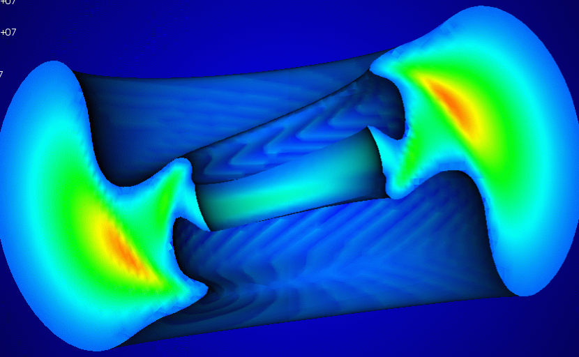
Figure 4a: Model t915H2. (a) Linear density profile (similar to Figure 2aa) at $t=470M\approx 10\tau_{orb}$. The black hole spin axis is tilted $15^{\circ}$ to the left of the $z$-axis. (b) Cumulative precession angle $\gamma$ and (c) tilt $\beta$ in radians as functions of radius. Initially, $\gamma=0$ and $\beta=15^{\circ}\approx 0.26$ throughout the disks. (d) Mass accretion rate in units of the Eddington mass accretion rate. (e) Transition radius (symbols) as a function of time along with the Lense-Thirring precession timescale $\tau_{LT}$, azimuthal sound crossing time $\tau_{cs}$, and accretion timescale $\tau_{acc}$. The thin vertical line marks the radius where $\tau_{LT}=\tau_{cs}$.

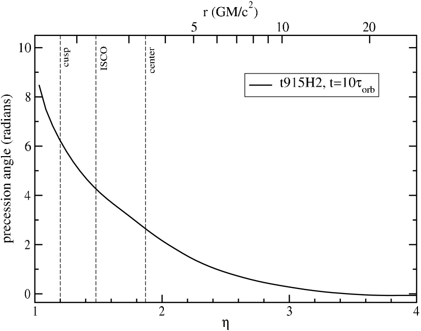
Figure 4b:

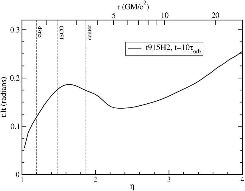
Figure 4c:

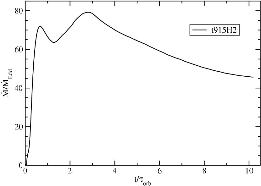
Figure 4d:

Figure 4e:

5.4 Models t930L & t930H

These models also begin from exactly the same initial conditions as Model t90 except that the black hole is tilted by an angle $\beta_{0}=30^{\circ}$. These models allow us to gauge how our results depend on the initial tilt of the disk. Model t930L uses a resolution of $48\times 24\times 48$ zones and is evolved until $t=1400M\approx 30\tau_{orb}$; Model t930H uses a resolution of $96\times 64\times 96$ and is evolved until $t=460M\approx 10\tau_{orb}$. Again there is very good agreement between the two.

These models have the highest accretion rates (Figure 5ad) of any considered. Again, this is expected since they begin with the disk furthest from equilibrium. One consequence of the very high accretion rate is that the disk is largely depleted of gas by the end of the simulation, particularly for the longer evolution of Model t930L, which was carried out to $t=1400M\approx 30\tau_{orb}$. Nevertheless, we find very similar results for the twist and tilt of these $\beta_{0}=30^{\circ}$ models compared with the previous $\beta_{0}=15^{\circ}$ models (compare Figures 5ac and 3ac). We again see the preferential accretion of highly tilted gas through two opposing streams starting near $r_{center}$. Again these streams cross near the symmetry plane of the black hole, leaving a small, nearly aligned ring of gas close to the horizon. These results further confirm that the mass accretion rate plays little, if any, role in regulating the precession or tilt of these disks.

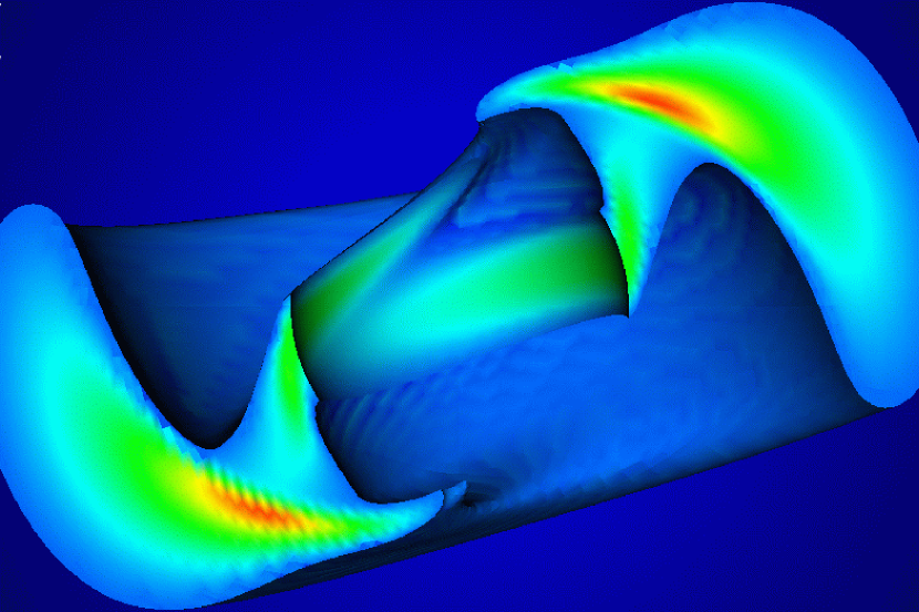
Figure 5a: Model t930L & t930H. (a) Linear density profile (similar to Figure 2aa) for Model t930H at $t=460M\approx 10\tau_{orb}$. The black hole spin axis is tilted $30^{\circ}$ to the left of the $z$-axis. (b) Cumulative precession angle $\gamma$ and (c) tilt $\beta$ in radians as functions of radius. Initially, $\gamma=0$ and $\beta=30^{\circ}\approx 0.52$ throughout the disks. (d) Mass accretion rate in units of the Eddington mass accretion rate. (e) Transition radius (symbols) as a function of time along with the Lense-Thirring precession timescale $\tau_{LT}$, azimuthal sound crossing time $\tau_{cs}$, and accretion timescale $\tau_{acc}$. The thin vertical line marks the radius where $\tau_{LT}=\tau_{cs}$.

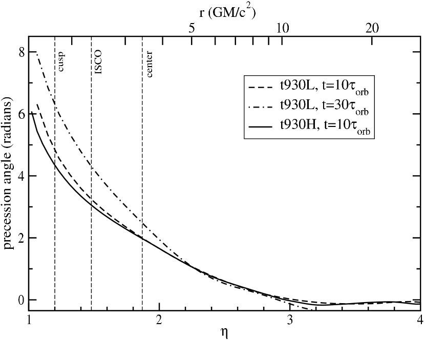
Figure 5b:

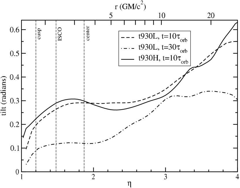
Figure 5c:

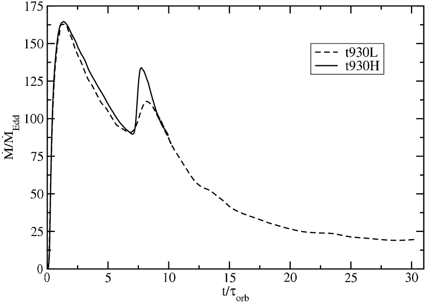
Figure 5d:

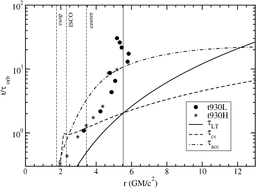
Figure 5e:

As in the previous models, the transition radius $r_{T}$ (Figure 5ae) asymptotes toward a radius $r_{T}\lesssim 6r_{G}$ consistent with the radius at which $\tau_{LT}\sim\tau_{cs}$. The early migration of $r_{T}$ is even similar to the previous models (compare Figures 5ae and 3ae). This leaves the larger accretion rate and tilt as practically the only differences between this and previous models. Thus, it appears our results are only weakly dependent on the initial tilt.

5.5 Model t915$\Gamma$

One of our general conclusions to this point is that differential Lense-Thirring precession in the disk is limited to radii for which $\tau_{LT}<\tau_{cs}$. However, this conclusion is based on a series of models that all share the same precession frequency and roughly the same sound speed in the disk. It is useful, therefore, to consider a model where at least one of these timescales is changed. In Model t915$\Gamma$, we use the same black-hole spin ($a/M=0.9$), disk parameters ($l/M=2.6088$ and $\Phi_{in}=-0.01$), and resolution ($48\times 24\times 48$) as Model t915L, except we change the equation of state of the gas such that $\Gamma=5/3$ and $\kappa=1.24\times 10^{5}$ (in cgs units). Since the sound speed in these models scales as $(\Gamma-1)^{1/2}$, this change increases the sound speed in the disk by $\sqrt{2}$ and decreases the azimuthal sound-crossing time by the same factor.

All other things being equal, our first expectation is that the faster sound speed in this disk should make the transition radius asymptote at a smaller value than in the previous models. Instead we see in Figure 6ab that the twist continues to grow with time throughout the disk. This is also apparent in Figure 6ae where the transition radius $r_{T}$ gradually moves outward in the disk throughout the entire simulation and does not asymptote toward a constant value. By the end of the simulation it reaches a value more than double the radius where $\tau_{LT}=\tau_{cs}$. Although this result seems surprising in light of what we found in the previous models, when considered within the context of the results presented below, it is apparent that Model t915$\Gamma$ is a transition model. In all of the previous models, the radius where $\tau_{LT}=\tau_{cs}$ lies outside of $r_{center}$; thus differential Lense-Thirring precession dominates the bulk of the disk material. In the models presented in the next two sections, the radius at which $\tau_{LT}=\tau_{cs}$ lies inside of $r_{center}$; those disks, therefore, have very efficient internal communication throughout the bulk of the disk and respond more uniformly to precession. For the current model, $r_{center}$ and the radius at which $\tau_{LT}=\tau_{cs}$ differ by less than $25$%; as a consequence, $\tau_{LT}\approx\tau_{cs}$ for the bulk of the disk material. This balance prevents either differential precession or wave propagation from dominating the evolution. As a result, in Figure 6ae we find an intermediate behavior between the vertical asymptote seen in strong differential precession models (Figures 3ae, 4ae, and 5ae) and the nearly horizontal limit of solid body precession (Figure 8ae).

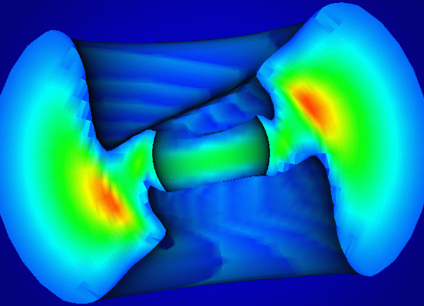
Figure 6a: Model t915$\Gamma$. (a) Linear density profile (similar to Figure 2aa) at $t=1400M\approx 30\tau_{orb}$. The black hole spin axis is tilted $15^{\circ}$ to the left of the $z$-axis. (b) Cumulative precession angle $\gamma$ and (c) tilt $\beta$ in radians as functions of radius. Initially, $\gamma=0$ and $\beta=15^{\circ}\approx 0.26$ throughout the disks. (d) Mass accretion rate scaled to allow direct comparison with our other models. (e) Transition radius (symbols) as a function of time along with the Lense-Thirring precession timescale $\tau_{LT}$, azimuthal sound crossing time $\tau_{cs}$, and accretion timescale $\tau_{acc}$. The thin vertical line marks the radius where $\tau_{LT}=\tau_{cs}$.

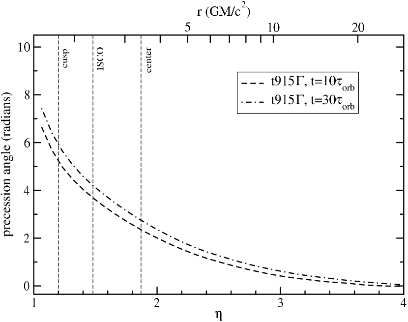
Figure 6b:

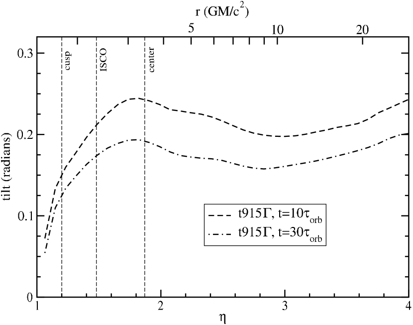
Figure 6c:

Figure 6d:

Figure 6e:

5.6 Model t915R

Model t915R explores a retrograde torus model. The magnitude of the black hole spin ($|a|=0.9$) is the same as in the previous models, but it spins in the opposite sense. Thus, the angular momentum of the black hole and torus are almost anti-parallel; they differ from anti-parallel by $15^{\circ}$. The retrograde orbit requires the torus to have a higher specific angular momentum to ensure $l>l_{ms}$. In this case, $l/M=4.4751$; the torus center is at $r_{center}/r_{G}=12$. The cusp in the potential is located at $r_{cusp}/r_{G}=6.67$, $\theta=\pi/2$ with $\Phi_{cusp}=-0.03$. We choose an inner surface potential $\Phi_{in}=-0.0125$ giving an energy gap $\Delta\Phi=0.0175$. The outer boundary is set at $r_{max}/r_{G}=80$ and the simulation is evolved until $t=2000M\approx 8\tau_{orb}$.

The most obvious thing we notice in Figure 7aa is that the accretion stream in this model takes the form of a relatively thin disk lying very close to the symmetry plane of the black hole. In this sense, the results appear very similar to the usual Bardeen-Petterson configuration, but for a very different physical reason as we shall see. The gas in the accretion stream still orbits in a retrograde sense just as the rest of the disk does. Therefore, the gas in the accretion stream has a tilt $\beta\approx\pi$ (Figure 7ac) consistent with retrograde motion near the symmetry plane of the black hole. Closest to the black hole ($\eta<1.6$; $r/r_{G}<2.62$), the accreting gas actually appears to tilt away from the symmetry plane. This is due the inclusion of background gas in our calculations. Close to the black hole, the background gas is undergoing very rapid prograde precession near the symmetry plane of the black hole. It, therefore, provides a $\beta\approx 0$ contribution near the black hole.

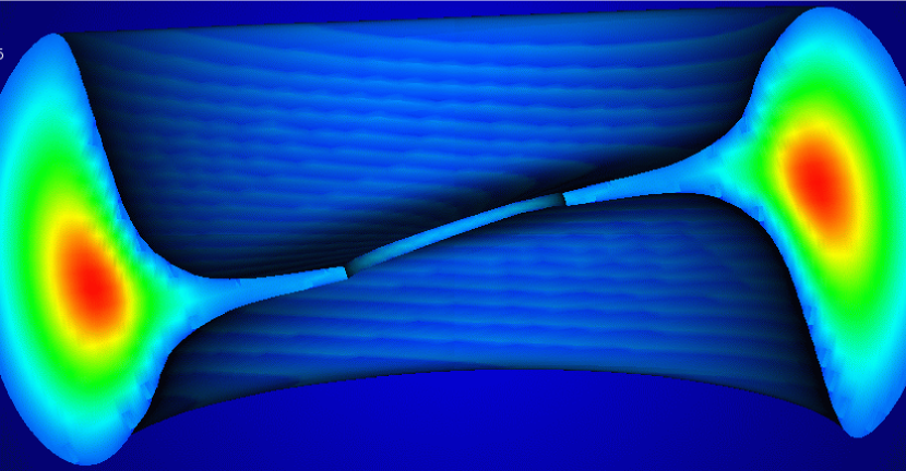
Figure 7a: Model t915R. (a) Linear density profile (similar to Figure 2aa) at $t=2000M\approx 8\tau_{orb}$. The black hole spin axis is tilted $15^{\circ}$ to the right of the $-z$-axis (points down and to the right). (b) Cumulative precession angle $\gamma$ and (c) tilt $\beta$ in radians as functions of radius. Initially, $\gamma=0$ and $\beta=165^{\circ}\approx 2.88$ throughout the disks. (d) Mass accretion rate in units of the Eddington mass accretion rate. (e) Transition radius (symbols) as a function of time along with the Lense-Thirring precession timescale $\tau_{LT}$, azimuthal sound crossing time $\tau_{cs}$, and accretion timescale $\tau_{acc}$. Here the thin vertical line marks $r=r_{cusp}$.

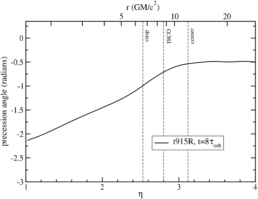
Figure 7b:

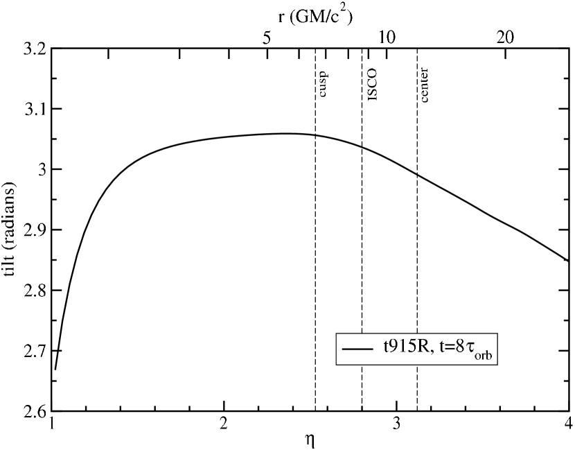
Figure 7c:

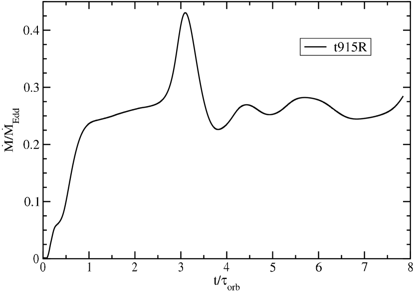
Figure 7d:

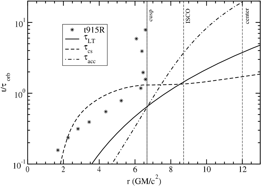
Figure 7e:

It is important to note that, within the accretion stream at $r<r_{cusp}$, the accretion timescale $\tau_{acc}$ is actually shorter than both the sound-crossing time $\tau_{cs}$ and the precession timescale $\tau_{LT}$ (Figure 7ae). We, therefore, don’t expect precession to have a dramatic effect at these small radii in this model since the Lense-Thirring precession timescale is longer than the dynamical timescale. The role of Lense-Thirring precession inside of $r_{cusp}$ is further diminished by the fact that most of the gas inside this radius lies very close to the symmetry plane of the black hole making precession essentially meaningless. Notice, for instance, that the calculation of the precession $\gamma$, which relies on the cross-product of $\mathbf{J}_{BH}$ and $\mathbf{J}_{Disk}$, which becomes unreliable whenever $\mathbf{J}_{BH}$ and $\mathbf{J}_{Disk}$ are nearly parallel or anti-parallel.

Outside of $r_{cusp}$, the accretion timescale becomes significantly longer, yet the sound-crossing time quickly becomes shorter than the precession timescale. Therefore, true differential precession is only expected to be important over a very small region in this disk model. Importantly though, we see in Figure 7ab that the precession proceeds in a retrograde fashion as expected (Lense-Thirring precession always proceeds in the direction of the black-hole spin). Precession also extends out to much larger radii (essentially throughout the disk) in this model than in previous models (see Figure 7ab). We will return to this point in the next section.

5.7 Model t515L & t515H

Model t515 explores the dependence of our results on the magnitude of the black hole angular momentum. For these models, the black hole has a spin $a/M=0.5$ and radius $r_{BH}/r_{G}=1.87$; the torus has a specific angular momentum $l/M=3.385$; the torus center is at $r_{center}/r_{G}=6.92$. The cusp in the potential is located at $r_{cusp}/r_{G}=2.96$, $\theta=\pi/2$ with $\Phi_{cusp}=-0.0136$. We choose an inner surface potential $\Phi_{in}=-0.0096$ giving an energy gap $\Delta\Phi=0.004$. The outer boundary is set at $r_{max}/r_{G}=120$. Model t515L uses a resolution of $48\times 24\times 48$ zones and is evolved until $t=2400M\approx 20\tau_{orb}$; Model t515H uses a resolution of $96\times 64\times 96$ and is evolved until $t=1200M\approx 10\tau_{orb}$. Since the grid in these models has a larger maximum radius than most of the other models, the effective resolution is somewhat less.

There are two striking features to these models. First, in Figures 8aa and c, we see that the inner accretion disk appears to tilt away from the symmetry plane of the black hole. This is actually consistent with what we have seen in previous models in the sense that the black hole preferentially accretes the most tilted material. As in previous models, two opposing accretion streams begin from latitudes well above and below the black-hole symmetry plane near $r_{center}$. The accretion streams in this model actually begin at comparable latitudes to what is seen in Model t915 (compare Figures 8aa and 3aa). Again, this material carries much of the tilted angular momentum into the hole and allows the disk to gradually align. Since the streams have a greater tilt on average than the material further out, $\beta$ increases toward smaller radii inside $r_{center}$ as seen in Figure 8ac. However, unlike our $a/M=0.9$ models, these accretion streams do not cross before passing into the hole and we do not see the formation of an inner ring of low $\beta$ material. Consequently, $\beta$ remains large from near $r_{center}$ all the way in to the horizon.

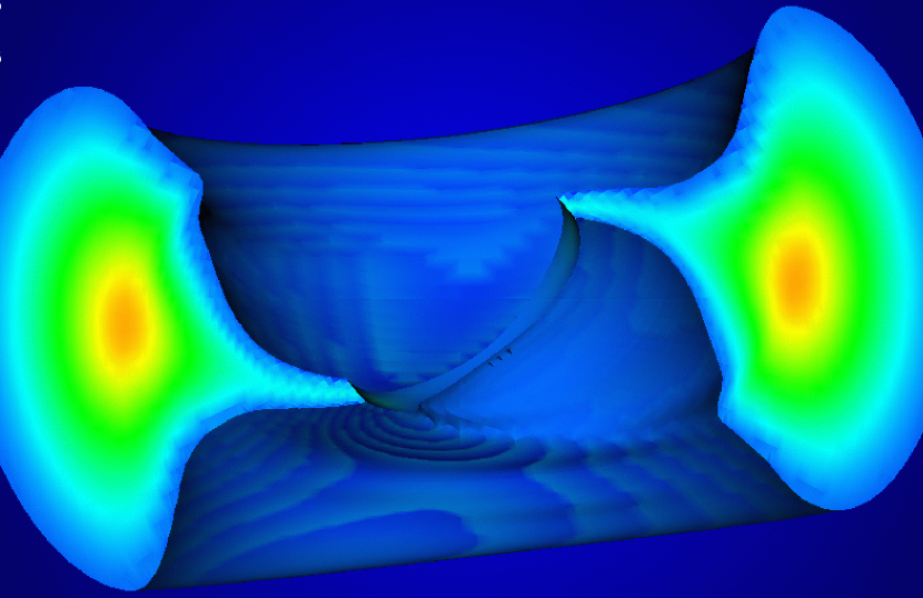
Figure 8a: Model t515. (a) Linear density profile (similar to Figure 2aa) at $t=1200M\approx 10\tau_{orb}$. The black hole spin axis is tilted $15^{\circ}$ to the left of the $z$-axis. (b) Cumulative precession angle $\gamma$ and (c) tilt $\beta$ in radians as functions of radius. Initially, $\gamma=0$ and $\beta=15^{\circ}\approx 0.26$ throughout the disks. In panel b, we have included data from $t=0.3$, 1, 1.6, 3.2, 6.4, and $8\tau_{orb}$ (dotted lines) to give a more complete time history of the precession. (d) Mass accretion rate in units of the Eddington mass accretion rate. (e) Transition radius (symbols) as a function of time along with the Lense-Thirring precession timescale $\tau_{LT}$, azimuthal sound crossing time $\tau_{cs}$, and accretion timescale $\tau_{acc}$. The thin vertical line marks the radius where $\tau_{LT}=\tau_{cs}$.

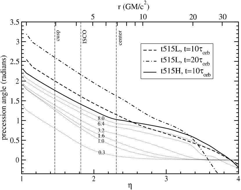
Figure 8b:

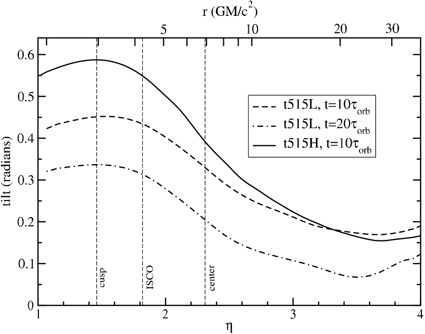
Figure 8c:

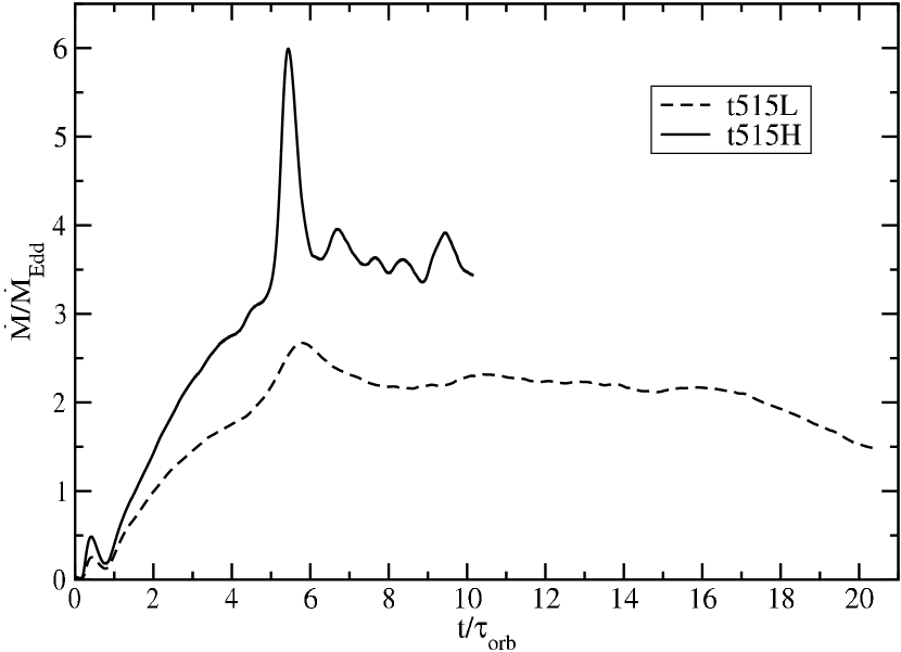
Figure 8d:

Figure 8e:

The second striking feature is apparent in Figure 8ae. Although the transition radius at first approaches an asymptotic value coincident with $\tau_{LT}\approx\tau_{cs}$ similar to our other models, it later appears to rapidly move outward with no sign of another limit being reached. This is actually evidence of near rigid-body precession in the disk. For pure rigid-body precession, the twist $\gamma$ in Figure 8ab would be a horizontal line and the transition radius would lose its meaning since there would be no “transition” from an inner, twisted region to an outer, untwisted one. Model t515 doesn’t quite undergo pure rigid-body precession. It actually starts out undergoing differential precession and then switches to near rigid-body precession. This change is most apparent in the time sequence of $\gamma$-profiles shown in Figure 8ab. This also explains the near constant precession angle for gas beyond $r=r_{center}$ in Figures 7ab.

Generally, rigid-body precession is expected in disks whenever $\tau_{cs}$ is less than the applicable precession timescale (Larwood et al., 1996), in this case whenever $\tau_{cs}<\tau_{LT}$. This condition is actually met in all of our models at large enough radii; however, only in Models t515 and t915R is this condition met for $r<r_{center}$. Thus, only in these two models does the bulk of the gas in the disk meet the condition for rigid-body precession.

6 Discussion and Summary

We have performed the first fully relativistic numerical studies of tilted accretion disks around Kerr black holes. Such disks are subject to Lense-Thirring precession, resulting in a torque that tends to twist and warp the disk. For the thick disks considered here, we find that the nature of this precession depends primarily on the sound speed in the disk. Whenever $\tau_{LT}<\tau_{cs}$ in the bulk of the disk, it undergoes differential precession out to a transition radius set by $\tau_{LT}\approx\tau_{cs}\lesssim\tau_{acc}$, which occurs at a relatively modest distance of $r/r_{G}\approx 7$. In other disk models, such as viscous Keplerian disks, this transition may occur at somewhat larger radii ($\sim 15-30r_{G}$, Nelson & Papaloizou, 2000). We find that the location of this transition radius does not depend strongly on the size, mass, mass accretion rate, or tilt of the disk. The initial tilt does, however, affect the overall mass accretion rate for our models, since higher tilt models begin further from equilibrium within the black hole potential.

Whenever $\tau_{LT}>\tau_{cs}$ for the bulk of the disk, we find that it undergoes near rigid-body precession after a short initial period of differential precession. Such rigid-body precession of a thick disk could have important astrophysical consequences. For instance, this is the basis of at least one model attempting to explain the 106 day variability observed from Sgr A* (Liu & Melia, 2002), the $2.6\times 10^{6}M_{\odot}$ black hole at the Galactic center. It could also be important for understanding the jet precession observed in Galactic microquasars such as SS 433 and Her X-1.

One obvious shortcoming of this work is that we have ignored angular momentum transport mechanisms that are likely present in most astrophysical disks [e.g. viscosity or the magneto-rotational instability (Balbus & Hawley, 1991)]. Angular momentum dissipation may allow the inner region of the tilted disk to align more quickly with the symmetry plane of the black hole than what we see in the inviscid disks considered here (Bardeen & Petterson, 1975; Kumar & Pringle, 1985; Scheuer & Feiler, 1996). The alignment may also be more efficient in viscous disks, resulting in a sharper transition (Nelson & Papaloizou, 2000). A sharp transition from an inner aligned disk to a tilted outer disk may be useful in explaining a variety of phenomena observed in black-hole systems, such as quasi-periodic oscillations (Fragile et al., 2001) as well as certain spectral features.

References

- Abramowicz et al. (1978) Abramowicz, M., Jaroszynski, M., & Sikora, M. 1978, A&A, 63, 221
- Anninos & Fragile (2003) Anninos, P., & Fragile, P. C. 2003, ApJS, 144, 243
- Balbus & Hawley (1991) Balbus, S. A., & Hawley, J. F. 1991, ApJ, 376, 214
- Bardeen & Petterson (1975) Bardeen, J. M., & Petterson, J. A. 1975, ApJ, 195, L65
- Bardeen et al. (1972) Bardeen, J. M., Press, W. H., & Teukolsky, S. A. 1972, ApJ, 178, 347
- De Villiers & Hawley (2002) De Villiers, J., & Hawley, J. F. 2002, ApJ, 577, 866
- De Villiers & Hawley (2003) De Villiers, J., & Hawley, J. F. 2003, ApJ, 592, 1060
- Elvis et al. (2002) Elvis, M., Risaliti, G., & Zamorani, G. 2002, ApJ, 565, L75
- Fishbone & Moncrief (1976) Fishbone, L. G., & Moncrief, V. 1976, ApJ, 207, 962
- Font & Daigne (2002) Font, J. A., & Daigne, F. 2002, MNRAS, 334, 383
- Font et al. (1998) Font, J. A., Ibáñez, J. M. ., & Papadopoulos, P. 1998, ApJ, 507, L67
- Fragile et al. (2001) Fragile, P. C., Mathews, G. J., & Wilson, J. R. 2001, ApJ, 553, 955
- Gammie et al. (2003) Gammie, C. F., McKinney, J. C., & Tóth, G. 2003, ApJ, 589, 444
- Gammie et al. (2004) Gammie, C. F., Shapiro, S. L., & McKinney, J. C. 2004, ApJ, 602, 312
- Hawley (1991) Hawley, J. F. 1991, ApJ, 381, 496
- Hawley et al. (1984) Hawley, J. F., Smarr, L. L., & Wilson, J. R. 1984, ApJS, 55, 211
- Igumenshchev & Beloborodov (1997) Igumenshchev, I. V., & Beloborodov, A. M. 1997, MNRAS, 284, 767
- Koide et al. (1999) Koide, S., Shibata, K., & Kudoh, T. 1999, ApJ, 522, 727
- Kozlowski et al. (1978) Kozlowski, M., Jaroszynski, M., & Abramowicz, M. A. 1978, A&A, 63, 209
- Kumar & Pringle (1985) Kumar, S., & Pringle, J. E. 1985, MNRAS, 213, 435
- Larwood et al. (1996) Larwood, J. D., Nelson, R. P., Papaloizou, J. C. B., & Terquem, C. 1996, MNRAS, 282, 597
- Lee & Kluźniak (1999) Lee, W. H., & Kluźniak, W. Ł. 1999, ApJ, 526, 178
- Liu & Melia (2002) Liu, S., & Melia, F. 2002, ApJ, 573, L23
- MacFadyen & Woosley (1999) MacFadyen, A. I., & Woosley, S. E. 1999, ApJ, 524, 262
- Natarajan & Pringle (1998) Natarajan, P., & Pringle, J. E. 1998, ApJ, 506, L97
- Nelson & Papaloizou (2000) Nelson, R. P., & Papaloizou, J. C. B. 2000, MNRAS, 315, 570
- Paczynsky & Wiita (1980) Paczynsky, B., & Wiita, P. J. 1980, A&A, 88, 23
- Papadopoulos & Font (1998) Papadopoulos, P., & Font, J. A. 1998, Phys. Rev. D, 58, 24005
- Papaloizou & Pringle (1984) Papaloizou, J. C. B., & Pringle, J. E. 1984, MNRAS, 208, 721
- Rees (1978) Rees, M. J. 1978, Nature, 275, 516
- Scheuer & Feiler (1996) Scheuer, P. A. G., & Feiler, R. 1996, MNRAS, 282, 291
- Vietri & Stella (1998) Vietri, M., & Stella, L. 1998, ApJ, 507, L45
- Volonteri et al. (2004) Volonteri, M., Madau, P., Quataert, E., & Rees, M. J. 2004, ApJ
- Wilson (1972) Wilson, J. R. 1972, ApJ, 173, 431
- Yu & Tremaine (2002) Yu, Q., & Tremaine, S. 2002, MNRAS, 335, 965
- Zanotti et al. (2003) Zanotti, O., Rezzolla, L., & Font, J. A. 2003, MNRAS, 341, 832