3-D Photoionization Structure and Distances of Planetary Nebulae I. NGC 6369

Abstract

We present the results of mapping the planetary nebula NGC 6369 using multiple long slit spectra taken with the CTIO 1.5m telescope. We create two dimensional emission line images from our spectra, and use these to derive fluxes for 17 lines, the H$\alpha$/H$\beta$ extinction map, the [SII] line ratio density map, and the [NII] temperature map of the nebula. We use our photoionization code constrained by these data to determine the distance, the ionizing star characteristics, and show that a clumpy hour-glass shape is the most likely three-dimensional structure for NGC 6369. Note that our knowledge of the nebular structure eliminates all uncertainties associated with classical distance determinations, and our method can be applied to any spatially resolved emission line nebula. We use the central star, nebular emission line, and optical+IR luminosities to show that NGC 6369 is matter bound, as about 70% of the Lyman continuum flux escapes. Using evolutionary tracks from Blöcker (1995) we derive a central star mass of about 0.65 M_⊙.

1 Introduction

The planetary nebula (PN) NGC 6369 – shown in Fig. 1 in the light of H$\alpha$ + N[II]$\lambda$658.4nm – is an object with a complex morphology, consisting of a main bright annulus of diameter 40″, and fainter, curved outer structures on two sides in the E-W direction. Deep narrow band H$\alpha$  and  N[II]$\lambda$6584 images of NGC 6369 were obtained by Corradi, Schönberner, Steffen, & Perinotto (2003) in a survey to look for faint outer halos around PNe. Apart from being deeper, their image is not significantly different from the one shown in Fig. 1, and no large faint halo was found.

The HST image of NGC 6369 available at http://heritage.stsci.edu/2002/25/index.html also shows the same main features as our image but has additional resolved details, and tags the H$\alpha$, [OIII]500.7nm, and [NII]658.4nm lines with the colors red, blue and green respectively. In the section on observational results we discuss this composite HST image in more detail.

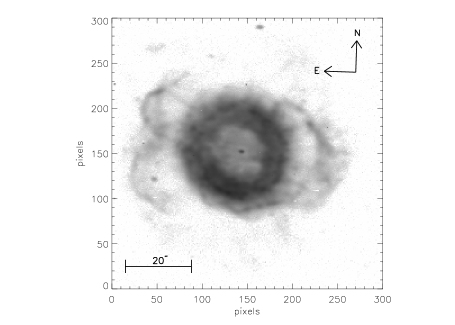
Figure 1: Narrow band filter image of NGC 6369 in H$\alpha$+[NII] from Schwarz, Corradi, & Melnick (1992). Note the bright ring and outer faint ansae to the E and W of the object. N is up, E to the left, and the plate scale is 0.26 ”/pix.

The equatorial and galactic coordinates for NGC 6369 are $\alpha$ = 17^h 29^m 20^s.40 and $\delta$ = 23^o 45′ 37″.9 (ICRS2000), and l = 2.43^o b = +5.85^o respectively. The extreme distances determined for NGC 6369 are 0.33 kpc obtained by Amnuel, Guseinov, Novruzova, & Rustamov (1984), and 2.00 kpc obtained by Gathier, Pottasch, & Goss (1986), out of a total of 10 listed by Acker et al. (1992), from which we obtain a mean value for the distance to NGC 6369 of 1039$\pm$ 538 pc. Note that these ten distances were determined using several statistical methods, each with their own systematic biases and assumptions, so that the average probably is a reasonably unbiased estimator, within the (large) error.

The temperature of the central star obtained from the Zanstra method by Gathier, & Pottasch (1989) is $T(H)_{\mathrm{Z}}=67\,600~{}\mathrm{K}$. The star has been classified as a WC4 star by Tylenda, Acker, & Stenholm (1993).

Spectra of NGC 6369 were obtained by Acker, Koppen, Stenholm, & Jasniewicz (1989), using an IDS (Image Dissector Scanner) as detector with double 4 ″ apertures, by Aller & Keyes (1987) using an ITS (Image Tube Scanner) with a $2\arcsec\,\times\,10\arcsec$ slit, and by Perinotto, Purgathofer, Pasquali, & Patriarchi (1994) using an IDS and a combination of different apertures not bigger than $13\arcsec\,\times\,13\arcsec$. An expansion velocity of $41.5$ km s^-1 has been determined by Meatheringham, Wood, & Faulkner (1988). The system radial velocity was reported to be -106 km.s^-1 by Wilson (1953), and -101 km.s^-1 by Meatheringham, Wood, & Faulkner (1988).

The spectral energy distribution (SED) of NGC 6369 is shown in Fig. 2 and has been computed using flux values from Acker et al. (1992) and Schmeja, & Kimeswenger (2002) over a range of wavelengths from 0.44 to 1100 $\mu$m. Note that we plot $\lambda$ F_λ against wavelength and below we will use the F_λ values to determine the observed optical+IR luminosity of NGC 6369.

Figure 2: The SED for NGC 6369 between 0.44 and 1100 $\mu$m using flux values from the literature (see text).

Planetary nebulae are generally classified according to their appearance, and such classification is then used for studies of the formation and evolution of these objects (for example (Balick, 1987)). Such a classification, based on the observed two dimensional (2-D) brightness distribution in a given line or lines can be quite misleading. This could be the case for NGC 6369, for which a round morphology is evident from the observed images. Different 3-D geometries can produce the same observed 2-D morphology as has been shown by Monteiro, Morisset, Gruenwald, & Viegas (2000). Furthermore, images produced by ions of different ionization degree can be very different, due to the radiation transfer within the nebulae. Only detailed modeling, which reproduces the brightness intensity distribution of different lines, as well other observed parameters, can provide more reliable information about the 3-D geometry of the gas distribution. The determination of the actual 3-D gas distribution in planetary nebulae is essential for understanding their formation and evolution, as well as that of the ionizing star.

By determining the 3-D structure of nebulae, we eliminate the large uncertainties that have plagued classical statistical distance determination methods for over 5 decades. Assumptions about the filling factor, constancy of ionized mass or diameter, mass-radius relationships etc. are not needed here: we know what the structure and ionized mass are, and can therefore determine distances to much greater accuracy than before. In this paper we explain in detail how we can determine this 3-D structure from long slit spectra and our 3-D photo-ionization model, and apply it to the case of NGC 6369

In summary, we obtain the spatial structure of the object along with its chemical composition, ionizing source temperature and luminosity, mass, as well as an independent distance, in a self-consistent manner. In §2 we discuss the observations and basic reduction procedures, as well as the details of the image reconstruction technique used to obtain the line intensity maps. In §3 the results obtained from these maps are discussed: the reddening correction of the images, total line fluxes and the computed temperature and density maps. In §4 we present the model results of the 3-D photoionization code, and we discuss the derived quantities Finally, in §5 we give our conclusions.

2 Observations and Mapping

2.1 Observations and general reduction

Observations were made using the CTIO 1.5 m Ritchey-Chrétien telescope with the RC Spectrograph on the nights of 12 and 13th June, 2002. We used a grating with 600 l/mm blazed at 600 nm giving a spectral resolution of 0.65 nm per pixel and a plate scale of 1.3″/pixel with a slit width of 4″. The spectral coverage obtained with this configuration was approximately 450 nm to 700 nm. We took three 1200s exposures at each slit position for ease of cosmic hit removal etc.. For details of the instrument and telescope see http://www.ctio.noao.edu and click on “Optical Spectrographs”, then on “1.5M RC spectrograph”.

By taking sets of exposures at several parallel long-slit positions across the nebula, we obtained line intensity profiles for each slit. These profiles were then combined to create emission line images of the nebula with a spatial resolution of about $4\arcsec\,\times\,4\arcsec$, in a way similar to radio mapping. This method has been applied before for the PN NGC 3132 as discussed in Monteiro, Gruenwald, Morisset, & Viegas (2002). A total of 10 positions were observed, moving the slit in 4″steps in the N-S direction between exposures. The third position observed from south to north (east is to the left, and north is up in all the figures) was not observed due to pointing problems. For this position an average of the two adjacent exposures was adopted.

The seeing conditions during the observing run were 1.5″or better, obtained from the seeing monitor at CTIO. In both nights the atmospheric conditions were photometric.

The individual slit spectra were reduced using standard procedures for long-slit spectroscopy, using IRAF reduction packages. The wavelength calibration was applied to the two dimensional images using the tasks FITCOORDS and TRANSFORM after re-identifying the arc spectra in many spatial positions. This procedure helps to remove distortions in the image that may be present due to slit curvature and misalignment with respect to the CCD. The final corrected images show displacements of the order of one pixel, which is the precision limit of this method. An additional fine correction for slit misalignment was made using the H$\alpha$ and H$\beta$ profiles for each exposure. Using IDL the images were re-dimensioned to 100 times their original size. The normalized H$\alpha$ and H$\beta$ profiles were then matched and the final result re-dimensioned to original values. This procedure yields the precise alignment necessary for calculation of diagnostic line intensity ratios. Minor shifts of the order of one pixel can introduce considerable errors in line ratios, if this method is not applied. The error introduced in line ratios by misalignments can reach 4% on sharp edges of the brightness profile.

For the flux calibrations two standard stars, LTT 7379 and LTT 9239 were observed on both nights. The final sensitivity function obtained from these stars, using the IRAF task SENSFUNC, has an RMS of 0.02, indicating the good photometric quality of the nights. Based on previous similar spectrophotometric observations made with the INT on La Palma, we compute the random error on individual line flux calibrations to be 3%, while the overall possible systematic uncertainty in the stellar flux is about 5%.

2.2 Image reconstruction

The final emission line images were obtained from the spatially integrated flux profile in each slit. To obtain the slit profile of integrated fluxes in a given transition, a Gaussian function was fitted to each point along the spatial direction using IDL routines. The errors adopted for the fits were the standard deviations calculated by the fitting procedure. The profiles for each slit position were then combined and interpolated using a cubic convolution algorithm (Park, & Schowengerdt, 1983; Rifman, & McKinnon, 1974), in order to reconstruct a 2-D image of the nebula for that transition. Integration of this final image provides the total observed flux for the nebula, for each line. Note that this procedure gives better estimates of the total flux and relative line intensities than observing just one slit position or aperture, since it takes into account the entire nebula.

Signal to noise images were also obtained using the fitted profiles by subtracting the fitted profile from the original section and analyzing the remaining noise. This is a combination of all noise sources in the image (photon statistics, noise introduced by the data reduction procedures, etc.). These errors were then combined with the fitting errors mentioned above, using the usual error propagation expressions to make the final signal to noise image. We then quadratically added the 3% random calibration error and the de-reddening error computed from the H$\alpha$/H$\beta$ reddening map (see §3.1), to arrive at the overall error for each line flux. This procedure provides precise error estimates for the total fluxes and diagnostic line ratio calculations.

3 Observational results

Images were created for all 17 lines detected with sufficient signal-to-noise ratio. In Fig. 3 the images for the most important lines are shown. The important [OIII]436.3nm line fell outside our available spectral range and could therefore not be included in our analysis. The images were corrected for reddening as described in the following section. The extracted total line intensities with their fractional total errors are given in Table 1.

Note that all main features are reproduced in these reconstructed line images. The outer ansae only show up in the [NII]685.4nm line, and are extremely faint or invisible in all other lines, as they are in the HST original images shown at http://heritage.stsci.edu/2002/25/original.html The [OIII]500.7nm emission comes mainly from the central part of the bright ring-like structure, while H$\alpha$ comes from further out, and the outermost part is dominated by [NII]685.4nm. Clearly, we do not reproduce the fine detail visible in the HST image because of our effective spatial resolution of 4” in the observational data. However, the expected ionization stratification for the different ions and the overall nebular structure are clearly seen in our images.

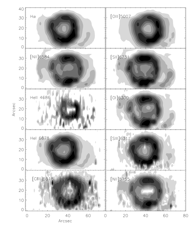
Figure 3: Reddening corrected, reconstructed emission line contour plots for NGC6369. The peak intensity in each frame is normalized to unity, and there are 7 contour steps between the maximum (black) and zero (white). N is up, E to the left.

3.1 Reddening correction and total fluxes

The reconstructed images for each line were corrected for reddening using the H$\alpha$/H$\beta$ ratio map shown in Fig. 4. The logarithmic correction constant was calculated pixel by pixel using the theoretical value of H$\alpha$/H$\beta$=2.87 ((Osterbrock, 1989)) and the reddening curve of Seaton (1979). We investigated the effect of differential atmospheric refraction on this ratio map. From the airmasses of our observed positions and the values given by Filippenko (1982) we computed a correction which we applied to our data. Since we used wide slits (4″) and the object is extended, the effect was small, but not negligible in the steep gradients near the bright ring structure. The average error due to this effect is about 2% in the high signal to noise areas and about 20% in the low signal to noise areas. The nett effect on the final calculated relative total fluxes is about 0.2% for strong lines and of 5% for weak ones, well within the other observed uncertainties.

In Fig. 5 we show the [NII]658.4nm image as an example before and after the reddening and differential refraction corrections.

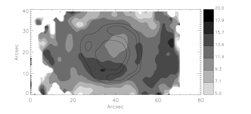
Figure 4: H$\alpha$/H$\beta$ ratio map with contour overlay of H$\alpha$ (Image is cut for S/N lower than 10). N is up, E to the left.

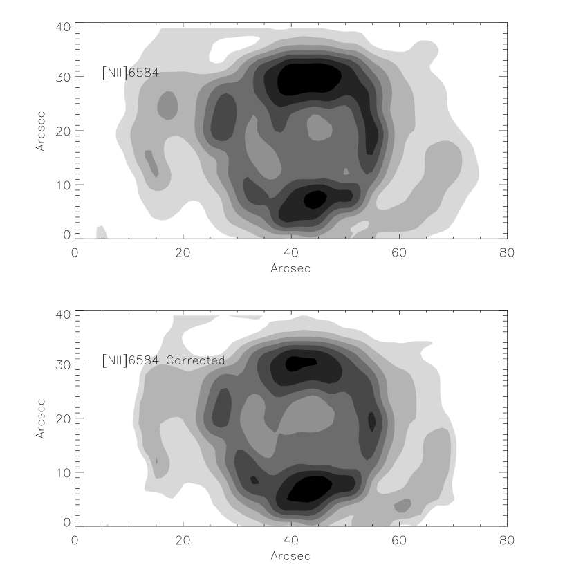
Figure 5: Comparison of [NII] image before and after reddening correction. N is up, E to the left.

The reddening correction was also obtained from the spatially integrated fluxes calculated from the images. The H$\alpha$ flux was divided by the H$\beta$ flux and a single value for the logarithmic extinction constant was obtained for the whole nebula. This value was then used to correct the total line intensities. The results for the line intensities were compared with those obtained from the first method and showed no differences to within the calculated uncertainties.

The resulting emission line fluxes relative to H$\beta$ and their corresponding total errors are shown in Table 1. All total fluxes were obtained by integrating the reddening corrected (pixel by pixel) images. The value we obtained for the total de-reddened H$\beta$ flux was $F_{H\beta}\,=\,7.2\,\times\,10^{-13}W\,m^{-2}$ and the uncorrected flux 5.9$\,\times\,10^{-15}W\,m^{-2}$ corresponding to a value of E(B-V) = 1.4 magnitudes.

Table 1: Line fluxes relative to H$\beta$

Line	Flux	Dered. Flux	Error (%)
HeII$\lambda$468.6	0.011	0.014	19
[OIII]$\lambda$495.9	4.59	4.11	7
[OIII]$\lambda$500.7	14.60	12.41	7
[CIII]$\lambda$551.8	0.01	0.01	25
[CIII]$\lambda$553.8	0.01	0.01	22
[NII]$\lambda$575.5	0.04	0.02	17
HeI$\lambda$587.6	0.47	0.16	8
[OI]$\lambda$630.0	0.22	0.05	8
[SIII]$\lambda$631.1	0.05	0.014	13
[OI]$\lambda$636.3	0.07	0.02	13
[NII]$\lambda$654.9	1.20	0.24	7
$H\alpha\lambda$656.3	13.80	2.87	7
[NII]$\lambda$658.4	3.70	0.73	7
HeI$\lambda$667.8	0.22	0.04	9
[SII]$\lambda$671.7	0.25	0.04	10
[SII]$\lambda$673.1	0.37	0.07	9

3.2 Gas density and temperature

We calculated the density and temperature maps from the reddening corrected maps of the [SII] and [NII] lines respectively. The expression relating the sulfur doublet line intensity ratios to the gas density is from de Robertis, Dufour, & Hunt (1987) which is also used in the IRAF package temden. The density map is shown in Fig. 6. For the temperature map we used the expression given by McCall (1984) as this allowed us to take the density variations over the nebula into account, which we did by using our density map. The difference between using this method and one that assumes constant density is small –since the temperature is only weakly dependent on the density– but systematic.

For the temperature maps, correction for slit misalignment was carried out as done for the H$\alpha$/H$\beta$ maps discussed in section 2.1. This correction was not necessary for the density maps since the small wavelength separation of the two lines generates very little deviation. The temperature map obtained after de-reddening is shown in Fig. 7(A). We also show the difference between the temperature map obtained using constant density and our map in Fig. 7(B). Note that the differences are less than 500 K. The images are clipped for data values with S/N lower than 10 for visual clarity.

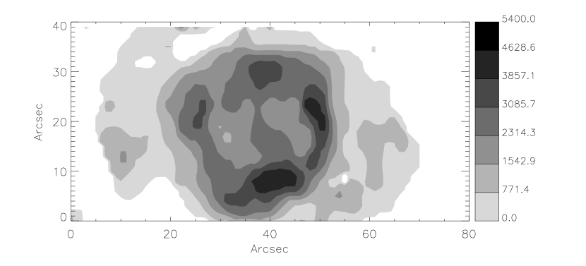
Figure 6: Density map obtained from the de-reddened [SII]671.7,673.1 line ratio using the method of de Robertis, Dufour, & Hunt (1987). N is up, E to the left.

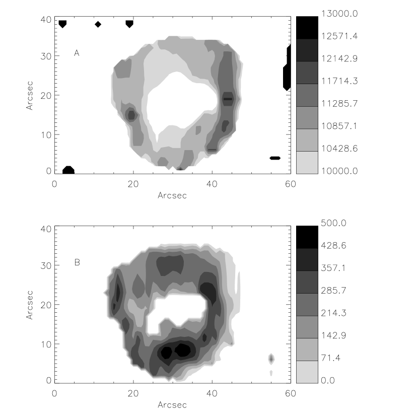
Figure 7: Temperature map obtained from the de-reddened [NII] line ratio (A), and the difference between this map and the one obtained using constant density (B). Note that the maximum difference is less than 500 K. N is up, E to the left.

3.3 Temperature of the central star

With the total fluxes corrected for interstellar reddening, the central star temperature can be calculated. For this, we apply the method described by Harman, & Seaton (1966), using the observed fluxes presented in §3.1 and the central star flux $F_{4793\AA}=1.20\,\times\,10^{-15}\,erg\,cm^{-2}\,s^{-1}$ obtained from Gathier, & Pottasch (1988). It is important to note that this method assumes spherical symmetry and a black-body spectral energy distribution for the ionizing star. This is not necessarily true as has been shown by many authors (for recent work see Rauch, Deetjen, Dreizler, & Werner (2000)) Here we use a blackbody spectrum modified by the major H and He absorption edges, and below we show by comparison with stellar evolution models from Blöcker (1995) that this is a reasonable method.

From the H$\beta$ and $HeII\lambda 468.6$ line fluxes, we obtain, respectively, $T_{\mathrm{Z}}(H)=70000~{}\mathrm{K}$ and $T_{\mathrm{Z}}(HeII)=106000~{}\mathrm{K}$. The value obtained for $T_{\mathrm{Z}}(H)$ with our fluxes differs slightly from the one obtained by Gathier, & Pottasch (1989) but is within the expected (large) uncertainties of the method. These values are more reliable than previously calculated ones since we have precise integrated fluxes for the whole nebula.

The Zanstra temperature for H and HeII are not necessarily equal, and do not correspond to the effective temperature of the central star if the nebula is not optically thick in all directions (Gruenwald, & Viegas, 2000). NGC 6369 is optically thin for radiation short-ward of 91.2 nm (Lyman continuum) since a rough estimate of the total luminosity in the optical lines is $\approx$ 14% of that shortward of 91.2 nm. Most of the UV escapes the nebula, and therefore we expect the T(H) do be lower than the T(He), as indeed found above.

4 Photoionization Models

The photoionization code applied here was described in detail by Gruenwald, Viegas, & Broguiere (1997). It uses a cube divided into cells, each having a given density. This allows arbitrary density distributions to be studied. The input parameters are the ionization source characteristics (luminosity, spectrum, and temperature), element abundances, density distribution, and the distance to the object. The conditions are assumed uniform within each cell where the code calculates the temperature and ionic fractions. These values are used to obtain emission line emissivities for each cell.

The final data cube can be oriented in order to reproduce the observed morphology. The orientation of the structure is thus also determined. The line intensities and other relevant quantities are then obtained after projection onto the plane of the sky. Note that because we lack velocity information, we cannot specify if an ansa is in front of or behind the main nebula.

The structure adopted for NGC 6369 is shown in Fig. 8 as it is oriented relative to the observer. The choice of the structure was based on the density map obtained from the observations. As shown in Monteiro, Morisset, Gruenwald, & Viegas (2000), closed shells were not able to reproduce the decrease in the density profile in the central regions of NGC 3132. For the same reason, we adopt an hour-glass shape for the main structure of NGC 6369, as its density map shows the same decrease in the central regions. We include random fluctuations in the density grid to simulate the clumpiness observed in images, as well as a density gradient along the main axis of the bipolar structure. The fluctuations were set to vary between the maximum and the minimum densities measured from the observational data. The rotation angles relative to the x, y and z axis are 70^o, 10^o, and 0^o respectively, with the symmetry axis of the main structure being x. The model resolution of $100^{3}$ cells was limited by computer memory.

The ionizing spectrum adopted for the central source is a modified blackbody with a break at 54.4eV. This was necessary to fit both the [OIII] and HeII line intensities, the last one being particularly sensitive to the depth of the break. This break is also present in the more precise theoretical atmospheric models presented by Rauch et al. (2003). The cutoff at 54.4 eV is one of the most prominent features that differentiates this spectrum from that of a blackbody, followed by the 13.6 eV hydrogen cutoff and absorption lines. The effective temperature and luminosity of this modified blackbody are listed in Table 2.

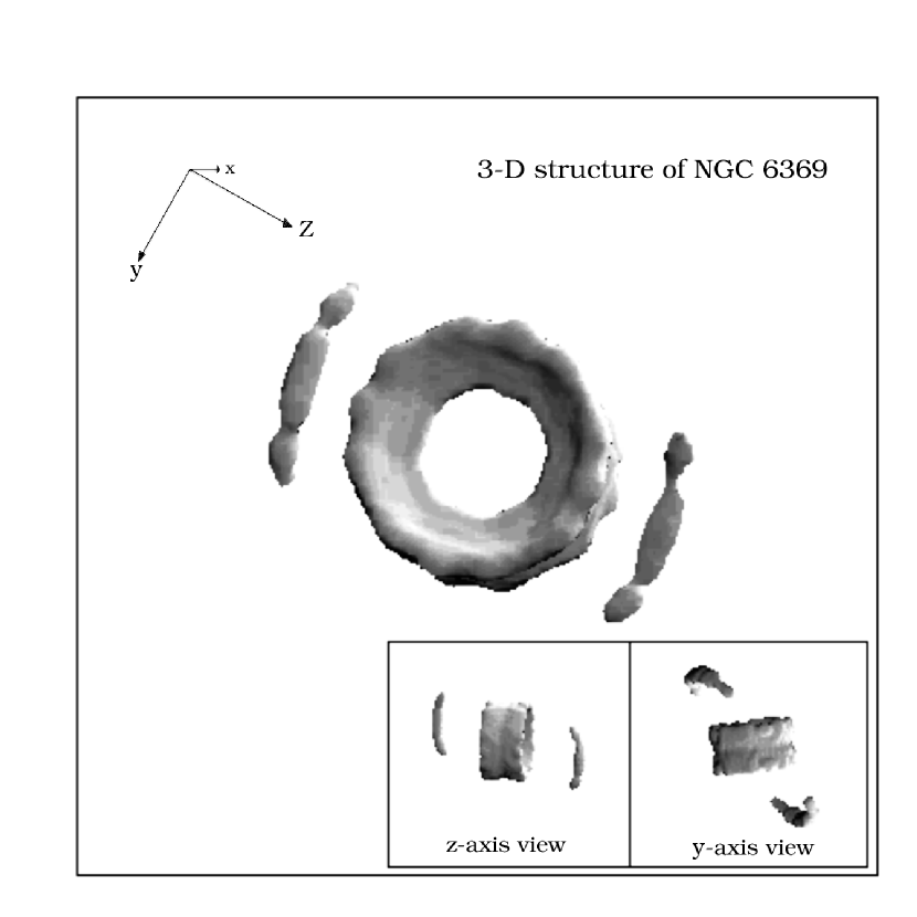
Figure 8: Iso-density plot of the 3-D structure used for the NGC 6369 model calculations. In the main image N is up, E to the left. The small insets view the structure along the other two axes, allowing the 3-D structure and orientation of the central object and the ansae to be clearly seen.

4.1 Model Results

We present here the main results obtained with the photoionization model. The total line intensities are given in Table 2, as well as the fitted abundances and ionizing star characteristics. Projected line images for the most important transitions are shown in Fig. 9.

The model image size is fitted to the observed size for the [NII]$\lambda 658.4\,nm$ line, as well as constrained by the absolute $H\beta$ flux. The distance of 1550 pc we determine is also constrained by fitting all the line fluxes and the shape of the nebula simultaneously, and for this reason is fundamentally different from classical distance determination methods, as it needs no assumptions to be made. One cannot increase the distance, and simply make the nebula larger to fit the optical image, as the line ratios would change significantly. 3-D ionization models such as this one cannot simply be scaled, thus placing much more stringent constraints on all derived parameters, including the distance. Note that this model distance is within one adjusted standard deviation of the average of all the observationally determined distances given in Sec. 1. Fig. 10 shows the observed [NII] image with the corresponding model image contours overlaid for the obtained distance.

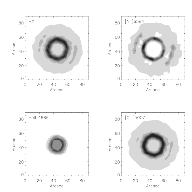
Figure 9: Projected line images obtained with the photoionization model. N is up, E to the left.

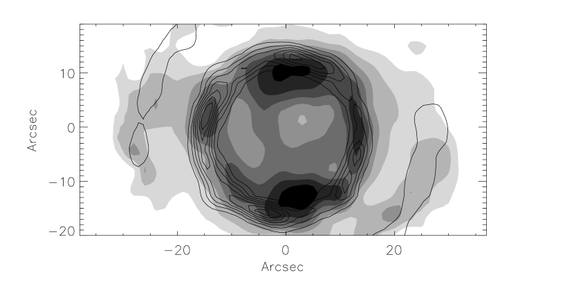
Figure 10: Contours of the model [NII] image over the observed image for d=1550 pc. N is up, E to the left.

Table 2: Observed and model line fluxes and model central star properties.

	Observed	Model
$T_{*}$ (K)	70kK-106kK	91kK
$L_{*}/L_{\odot}$	-	8100
Density	1000-5400	300-5400
He/H	-	$1.14\times 10^{-1}$
C/H	-	$3.3\times 10^{-4}$
N/H	-	$1.0\times 10^{-4}$
O/H	-	$6.1\times 10^{-4}$
Ne/H	-	$6.5\times 10^{-5}$
S/H	-	$7.5\times 10^{-6}$
log($H\beta$)	-12.14	-12.16
[NeIII]386.8a	0.9	0.9
[NII]658.4	0.73	0.78
[OIII]500.7	12.41	12.33
HeII468.6	0.014	0.013
HeI587.6	0.163	0.169
[OI]630.0	0.052	0.048
[SII]671.7	0.044	0.047
[SII]673.1	0.066	0.063

^a Value obtained from Peña, Stasińska, & Medina (2001)

The [SII] ratio map obtained with the model is shown in Fig. 11.

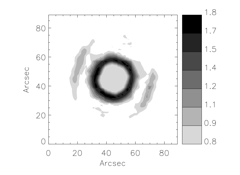
Figure 11: The [SII] line ratio obtained with the model. N is up, E to the left.

5 Discussion and conclusions

We have presented spectrophotometric maps of NGC 6369. These maps provided spatially resolved information for many emission lines and precise total fluxes for the whole nebula. The images produced with this technique were used to study the nebula with the usual diagnostic ratios. Each image was corrected for reddening pixel by pixel using the H$\alpha$/H$\beta$ image. This correction lead to some significant differences between the corrected and uncorrected images, as was shown in Figs. 5 & 7.

The H$\alpha$/H$\beta$ map shows some interesting features. In Fig. 4 we show that the extinction is not uniform across the nebula, as it varies between 6 and 18. The structure follows the main nebular morphology, which could indicate that dust and neutral material are present. This is to be expected since the nebula shows a very clumpy structure, which may cause shadowing within the gas, allowing for the survival of grains and neutral material. The prominent features on either side of the nebula do not show significant differences in extinction when compared to the main region.

The temperature map derived from the observed integrated line of sight intensities showed some structure but due to the low signal to noise ratio, this should be treated with caution. Within the errors and resolution of our observations the temperature can be considered to be constant across the nebula.

We also show that the density map indicates a decrease in density for the central regions. This decrease, as has been discussed by Monteiro, Morisset, Gruenwald, & Viegas (2000), is not compatible with a closed shell structure. Based on this map we propose an hour-glass structure for the main nebula, which has reproduced all the observational features of NGC 6369. This indicates that the one needs to use the [SII] ratio in addition to images to distiguish between open and closed structures.

The position of the outer condensations or ansae –which are off-set by 30^o from the main nebular symmetry axis– was obtained by matching model images with the observed line images (Fig. 3) as well as matching the model [SII] density map with the observed map (Fig. 6). The presence of these condensations can be accounted for by earlier ejection of matter and precession can account for their deviation from the symmetry axis. Many authors have dealt with these issues; for more complete discussions and models see for example Cliffe, Frank, & Jones (1996), Cliffe, Frank, Livio, & Jones (1995), García-Segura (1997), and Livio, & Pringle (1997).

Some of the parameters we have derived (and use as a sanity check) are:

The total luminosity of the observed lines, L_l = 1150 L_⊙; that derived from the SED by integrating the F_λ curve, L_o = 7.1$\,\times$ 10^-4 d² where d is the distance to NGC 6369 in pc, resulting in L_o = 1700 L_⊙ . Correcting this value using the method of Myers et al. (1987) we obtain 2550 L_⊙. The luminosity of the central star is L_tot = 8100 L_⊙ so that the ratios of the line and optical+IR luminosities to the total luminosity are respectively: L_l/L_tot = 0.14 and L_o/L_tot = 0.3. Assuming that the absorbed flux is re-radiated in the IR, mainly the IRAS bands, the integrated optical+IR luminosity indicates that about 70% of the UV flux (Lyman continuum) escapes from the nebula. This is not implausible as the nebula is open at it’s “poles” and is clumpy, allowing the radiation to pass through the many “holes”.

From the input matter distribution and abundances used in the model, we calculate the mass of the nebular ionized gas to be $M_{neb}\,=\,1.8\,M_{\odot}$. If we now use our values of luminosity and temperature for the central star and compare them with the evolutionary models of Blöcker (1995) we can obtain the mass of the central core. Using this procedure we can see from Fig. 12 that the best fitting track for our data corresponds to a mass somewhat higher than $M_{core}\,=\,0.625M_{\odot}$, say, $\approx\,0.65\,M_{\odot}$, and to an initial mass of $M_{0}=3M_{\odot}$. If we sum our nebular and core masses, we obtain $M_{core}\,+\,M_{neb}\,=\,2.4\,M_{\odot}$ approximately. If we use the line intensity errors as a measure of the goodness of the model results and combine the luminosity and temperature errors we obtain approximately 20-25% for the uncertainty in $M_{core}\,+\,M_{neb}$, placing the obtained initial stellar mass within the uncertainty of our determination. The value for $M_{neb}$ calculated from the model input density is a lower limit estimate of the total nebular mass as at least some material is present in the form of dust, as indicated qualitatively by our extinction map structure. Additionally, there may be neutral gas for wich we have no constraints.

Note that typical parameters for a WC4 PN central star from Allen, (1964) are T = 90kK, and R = 0.4 R_⊙, very close to our derived values of 91000 K and 0.4 R_⊙. Using g = G . M / R² in CGS units, we obtain log(g) = 5.1, which is much lower than the value of 5.8 derived from the depth of our He break. This is due to the fact that the central star has an extended atmosphere, again showing the consistency of the model results.

Figure 12: Comparison of model temperature and luminosity obtained for the central star with model tracks calculated by Blöcker (1995).

Using our photoionization code and the proposed structure we obtained a complete 3-D model for the NGC 6369. The fitted model line intensities show excellent agreement with the observed values. The obtained distance of d=1550 pc, is well within the range present in the literature obtained from different methods. The model temperature for the ionizing star is similar to the Zanstra (He) value discussed in §3.3. The temperature and luminosity values obtained from the model as well as the total nebular plus central star mass show good agreement with the stellar evolution models of Blöcker (1995).

Using multiple long slit spectroscopy, we can determine accurate distances, 3-D structures, abundances, ionized masses, central star masses, luminosities, and temperatures to any spatially resolved emission line nebula, assuming there are no strong shocks or extreme morphologies involved.

References

- Acker, Koppen, Stenholm, & Jasniewicz (1989) Acker, A., Koppen, J., Stenholm, B., & Jasniewicz, G. 1989, A&AS, 80, 201
- Acker et al. (1992) Acker, A., Ochsenbein, F., Stenholm, B., Tylenda, R., Marcout, J., & Schohn, C. 1992, Strabourg-ESO Catalogue of Galactic PNe.
- Allen, (1964) Allen, C. W., 1964 AQ, p216
- Aller & Keyes (1987) Aller, L. H., & Keyes, C. D. 1987, ApJS, 65, 405
- Amnuel, Guseinov, Novruzova, & Rustamov (1984) Amnuel, P. R., Guseinov, O. K., Novruzova, K. I. & Rustamov, I. S.1984, ApSS, 107, 19
- Balick (1987) Balick, B. 1987, AJ, 94, 671
- Blöcker (1995) Blöcker, T. 1995, A&A, 299, 755
- Cliffe, Frank, & Jones (1996) Cliffe, J. A., Frank, A., & Jones, T. W. 1996, MNRAS, 282, 1114
- Cliffe, Frank, Livio, & Jones (1995) Cliffe, J. A., Frank, A., Livio, M., & Jones, T. W. 1995, ApJ, 447, 49
- Corradi, Schönberner, Steffen, & Perinotto (2003) Corradi, R. L. M., Schönberner, D., Steffen, M., & Perinotto, M. 2003, MNRAS, 340, 417
- de Robertis, Dufour, & Hunt (1987) de Robertis, M. M., Dufour, R. J., & Hunt, R. W. 1987, JRASC, 81, 195
- Filippenko (1982) Filippenko, A. V. 1982, PASP, 94, 715
- García-Segura (1997) García-Segura, G. 1997, ApJ, 489, L189
- Gathier, Pottasch, & Goss (1986) Gathier, R., Pottasch, S. R., & Goss, W. M. 1986, AAp, 157, 191
- Gathier, & Pottasch (1988) Gathier, R., & Pottasch, S. R. 1988 , A&A, 197, 266
- Gathier, & Pottasch (1989) Gathier, R., & Pottasch, S. R. 1989, A&A, 209, 369
- Gruenwald, Viegas, & Broguiere (1997) Gruenwald, R., Viegas, S. M., & Broguiere, D. 1997, ApJ, 480, 283
- Gruenwald, & Viegas (2000) Gruenwald, R., & Viegas, S. M. 2000, ApJ, 543, 889
- Harman, & Seaton (1966) Harman, R.F., & Seaton, M. J. 1966, MNRAS, 132, 15
- Livio, & Pringle (1997) Livio, M., & Pringle, J. E. 1997, ApJ, 486, 835
- McCall (1984) McCall, M. L. 1984, MNRAS, 208, 253
- Meatheringham, Wood, & Faulkner (1988) Meatheringham, S. J., Wood, P. R., & Faulkner, D. J. 1988, ApJ, 334, 862
- Monteiro, Gruenwald, Morisset, & Viegas (2002) Monteiro, H., Gruenwald, R., Morisset, C., & Viegas, S. M. 2002, Revista Mexicana de Astronomía y Astrofísica Conference Series, 12, 170
- Monteiro, Morisset, Gruenwald, & Viegas (2000) Monteiro, H., Morisset, C., Gruenwald, R., & Viegas, S. M. 2000, ApJ, 537, 853
- (25) Myers, P.C. et al. 1987, ApJ, 319, 340
- Osterbrock (1989) Osterbrock, D. E. 1989, Research supported by the University of California, John Simon Guggenheim Memorial Foundation, University of Minnesota, et al. Mill Valley, CA, University Science Books, 1989, 422 p.,
- Peña, Stasińska, & Medina (2001) Peña, M., Stasińska, G., & Medina, S. 2001, A&A, 367, 983
- Perinotto, Purgathofer, Pasquali, & Patriarchi (1994) Perinotto, M., Purgathofer, A., Pasquali, A., & Patriarchi, P. 1994, A&AS, 107, 481
- Rifman, & McKinnon (1974) Rifman, S.S., & McKinnon, D.M., ”Evaluation of Digital Correction Techniques for ERTS Images; Final Report”, Report 20634-6003-TU-00, TRW Systems, Redondo Beach, CA, July 1974
- Rauch, Deetjen, Dreizler, & Werner (2000) Rauch, T., Deetjen, J. L., Dreizler, S., & Werner, K. 2000, Asymmetrical Planetary Nebulae II: From origins to microstructures, ASP Conference Series 199, 337
- Park, & Schowengerdt (1983) Park, S., & Schowengerdt, R. 1983 ”Image Reconstruction by Parametric Cubic Convolution”, Computer Vision, Graphics & Image Processing 23, 256
- Schmeja, & Kimeswenger (2002) Schmeja, S., & Kimeswenger, S. 2002, Revista Mexicana de Astronomía y Astrofísica Conference Series, 12, 176
- Schwarz, Corradi, & Melnick (1992) Schwarz, H. E., Corradi, R. L. M., & Melnick, J. 1992, AApS, 96, 23
- Seaton (1979) Seaton, M. J. 1979, MNRAS, 187, 73
- Tylenda, Acker, & Stenholm (1993) Tylenda, R., Acker, A., & Stenholm, B. 1993, AApS, 102, 595
- Wilson (1953) Wilson, R. E., 1953, GCRV, Carnegie Inst. Publ. 601