ROSAT-SDSS Galaxy Clusters Survey.

Abstract

For a detailed comparison of the appearance of cluster of galaxies in X-rays and in the optical, we have compiled a comprehensive database of X-ray and optical properties of a sample of clusters based on the largest available X-ray and optical surveys: the ROSAT All Sky Survey (RASS) and the Sloan Digital Sky Survey (SDSS). The X-ray galaxy clusters of this RASS-SDSS catalog cover a wide range of masses, from groups of $10^{12.5}$ $M_{\odot}$ to massive clusters of $10^{15}$ $M_{\odot}$ in the redshift range from 0.002 to 0.45. The RASS-SDSS sample comprises all the X-ray selected objects already observed by the Sloan Digital Sky Survey (114 clusters). For each system we have uniformly determined the X-ray (luminosity in the ROSAT band, bolometric luminosity, center coordinates) and optical properties (Schechter luminosity function parameters, luminosity, central galaxy density, core, total and half-light radii). For a subsample of 53 clusters we have also compiled the temperature and the iron abundance from the literature. The total optical luminosity can be determined with a typical uncertainty of 20% with a result independent of the choice of local or global background subtraction. We searched for parameters which provide the best correlation between the X-ray luminosity and the optical properties and found that the z band luminosity determined within a cluster aperture of 0.5 Mpc $\rm{h}_{70}^{-1}$ provides the best correlation with a scatter of about 60-70%. The scatter decreases to less than 40% if the correlation is limited to the bright X-ray clusters. The resulting correlation of $L_{X}$ and $L_{op}$ in the z and i bands shows a logarithmic slope of 0.38, a value not consistent with the assumption of a constant $M/L$. Consistency is found, however, for an increasing M/L with luminosity as suggested by other observations. We also investigated the correlation between $L_{op}$ and the X-ray temperature obtaining the same result.

1 Introduction

Cluster of galaxies are the largest well defined building blocks of our Universe. They form via gravitational collapse of cosmic matter over a region of several megaparsecs. Cosmic baryons, which represent approximately 10-15% of the mass content of the Universe, follow dynamically the dominant dark matter during the collapse. As a result of adiabatic compression and of shocks generated by supersonic motions, a thin hot gas permeates the cluster gravitational potential. For a typical cluster mass of $10^{14}$ $M_{\odot}$ the intracluster gas reaches a temperature of the order of $10^{7}$ keV and, thus, radiates optically thin thermal bremsstrahlung and line radiation in the X-ray band. In 1978, the launch of the first X-ray imaging telescope, the Einstein observatory, began a new era of cluster discovery, as clusters proved to be luminous ($\geq 10^{42-45}$ ergs $\rm{s}^{-1}$), extended ($\rm{r}\sim 1-5$ Mpc) X-ray sources, readily identified in the X-ray sky. Therefore, X-ray observations of galaxy clusters provide an efficient and physically motivated method of identification of these structures. The X-ray selection is more robust against contamination along the line of sight than traditional optical methods since the richest clusters are relatively rare and since X-ray emission, which is proportional to the gas density squared, is far more sensitive to physical overdensities than in the projected number density of galaxies in the sky. In fact the existence of diffuse, very hot X-ray emitting gas implies the existence of a massive confining dark matter halo. Moreover, selection according to X-ray luminosity is also an efficient way to find the highest mass concentrations due to well defined correlation between the X-ray luminosity and the total cluster mass (Reiprich & Bhöringher. 2002). In addition to allowing the identification of galaxy clusters, X-ray observations provide a wealth of information on the intracluster medium itself, e.g. its metal abundance, radial density distribution and temperature profile. These latter quantities, in turn, can be used to reliably estimate the total mass of the system.

In addition to the hot, diffuse component, baryons are also concentrated in the individual galaxies within the cluster. These are best studied through photometric and spectroscopic optical surveys, which provide essential information about luminosity, morphology, stellar population and age. Solid observational evidences indicate a strong interaction between the two baryonic components, as galaxies pollute the intracluster medium expelling metals via galactic winds producing the observed metal abundances in clusters (De Grandi et al. 2002, Finoguenov et al. 2001). On the other hand, the evolution of galaxies in clusters is influenced by processes due to the hot gas (e.g. gas stripping by ram pressure, etc.) as it is by internal processes like star formation, galactic winds, supernovae explosions etc., operating inside galaxies themselves (Dressler et al. 1997, Fasano et al. 2000, van Dokkum et al. 2000, Lubin et al. 2002, Kelson et al. 1997,2000, Ziegler&Bender 1997, Gomez et al. 2003). In conclusion, understanding the complex physics at play in clusters of galaxies requires combined X-ray and optical observation of a statistically significant sample of these objects.

On the basis of these considerations, we have created a large database of clusters of galaxies based on the largest available X-ray and optical surveys: the ROSAT All Sky Survey (RASS), the only X-ray all sky survey ever realized using an imaging X-ray telescope, and the Sloan Digital Sky Survey (SDSS), which is observing the whole Northern Galactic Cap and part of the Southern Galactic Cap in five wide optical bands covering the entire optical range. By carefully combining the data of the two surveys we have created the RASS-SDSS galaxy cluster catalog. Although two galaxy cluster catalogs from the SDSS already exist, the Cut and Enhance Galaxy Cluster Catalog of Goto et al. (2002) and the Merged Cluster Catalog of Bahcall et al. (2003, see also Kim et al. 2002), we prefered to compile a new cluster catalog by selecting the systems in the X-ray band, for which we have reliable X-ray characteristics and for the reasons explained above. The X-ray-selected galaxy clusters cover a wide range of masses, from groups of $10^{12.5}$ $M_{\odot}$ to massive clusters of $10^{15}$ $M_{\odot}$ in a redshift range from 0.002 to 0.45. The RASS-SDSS sample comprises all the X-ray detected objects already observed in the sky region covered by the Sloan Digital Sky Survey.

One of the first goals is the comparison of the X-ray and the optical appearance of the clusters. We want in particular find optical parameters that provide the closest correlation to the X-ray parameters, such that we can predict within narrow uncertainty limits the X-ray luminosity from these optical parameters and vice versa. So far optical and X-ray cluster surveys have been conducted independently without much intercomparison. Therefore, the empirical relationship between the X-ray luminosity and optical luminosity of clusters is not so well defined, in large part because of the difficulties inherent in measuring the cluster optical luminosity and in getting a homogeneous set of total optical luminosities for a large number of clusters. Edge and Stewart (1991) found that the bolometric X-ray luminosity of a local sample of X-ray-selected clusters correlated very roughly with Abell number and somewhat better with the Bahcall galaxy density (number of bright galaxies within 0.5 $\rm{h}^{-1}$ Mpc; Bahcall 1977,1981) for the small subsample that had Bahcall galaxy densities. Arnaud et al. (1992) made an heroic effort in computing cluster optical luminosities at low redshift from a heterogenous literature. The first joint X-ray/optical survey of galaxy clusters was the ROSAT Optical X-ray Survey (ROXS, Donahue et al. 2002). They observed 23 ROSAT pointings for a total of 5 square degrees in the I band and partially in the V band. The X-ray selection and the optical selection of cluster candidates were done independently, with the wavelets algorithm in the former case and with a matched filter algorithm in the latter one. They found X-ray and optical coincident detections for 26 galaxy clusters. Donahue et al. (2001) studied the relation between the X-ray luminosity and the matched filter parameter $\Lambda_{cl}$, which is approximately equivalent to the number of $L^{*}$ galaxies in the system (Postman et al. 1996). They found a marginally significant correlation between the two quantities with a significant scatter. Yee and Ellingson (2003) defined a new richness parameter as the number of cluster galaxies within some fixed aperture, scaled by a luminosity function and a spatial distribution function. They analysed a sample of 15 clusters from CNOC1 Cluster Redshift Survey, and found a very poor correlation between this parameter and other cluster properties such as the X-ray luminosity, temperature and the velocity dispersion.

In the present paper we describe the properties and the information contained in the RASS-SDSS catalog and the resulting correlations between the X-ray and optical properties in the sample. In section 2 we explain how the cluster sample has been created by X-ray selecting the systems from the available X-ray cluster and group catalogs. In section 3 we describe the method for calculating the X-ray cluster properties. We describe in section 4 the optical data and in section 5 the data reduction method. We analyse and discuss the correlations between the optical luminosity and the X-ray properties in section 6. We summarize and discuss the catalog properties and the results in section 7.

For all derived quantities, we have used $\rm{H}_{0}=70$ $\rm{km}$$\rm{s}^{-1}$$\rm{Mpc}^{-1}$, $\Omega_{m}=0.3$ and $\Omega_{\lambda}=0.7$.

2 The construction of the sample.

In order to correlate optical and X-ray galaxy cluster properties it is necessary to have a large statistical sample and to cover the whole mass range of the systems considered. Since the X-ray observations provide a robust method of identification of galaxy clusters and the X-ray luminosity is a good estimator of the system total mass, in principle the best approach should be constructing a cluster catalog of X-ray selected objects in a wide range of X-ray luminosity. While for intermediate and high X-ray luminosity (mass), several complete catalogs of X-ray selected clusters already exist (NORAS and REFLEX), in the low mass range a systematic X-ray survey of groups has still to be carried out. As a consequence, it is impossible at the moment constructing a strictly X-ray selected cluster sample, which covers a wide range of masses from very poor groups to rich clusters. A reasonable compromise in order to fill the low mass range of the spectrum is to select all the low mass clusters and groups to date X-ray detected, even if they are selected in other wavebands. This compromise is acceptable for our purposes, since we do not want to carry out an X-ray survey of galaxy clusters, but a systematic analysis of the correlation between X-ray and optical properties of those systems.

By following these criteria, the intermediate mass and high mass clusters have been selected from three ROSAT based cluster samples: the ROSAT-ESO flux limited X-ray cluster sample (REFLEX, Böhringer et al. 2003), the Northern ROSAT All-sky cluster sample (NORAS, Böhringer et al. 2000) and the NORAS 2 cluster sample (Retzlaff 2001) . REFLEX is a complete sample of clusters detected in 13924 $\rm{deg}^{2}$ in the southern hemisphere down to a flux limit of 3 $10^{-12}$ $\rm{erg}\rm{s}^{-1}\rm{cm}^{-2}$ in the $0.1-2.4$ $\rm{keV}$ comprising 448 clusters. The NORAS galaxy cluster survey contains 495 clusters showing extended emission in the RASS in the northern hemisphere with count rates $C_{X}\geq 0.06$ $\rm{counts}$ $\rm{s}^{-1}$ in the $0.1-2.4$ keV. NORAS 2 is the continuation of the NORAS project and aims at a complete survey of X-ray galaxy clusters, in 13598 $\rm{deg}^{2}$ of the northern hemisphere, down to a flux limit of $2$ $10^{-12}$ $\rm{erg}$ $\rm{s}^{-1}\rm{cm}^{-2}$ in the same X-ray band, which gives rise to an expected total of about 800 clusters. The samples are based on an MPE internal X-ray source catalog extracted with a detection likelihood $\geq 7$.

The low mass clusters and the groups have been selected from two catalogs of X-ray detected objects: the ASCA Cluster Catalog (ACC) from Horner et al. (2001) and the Group Sample (GS) of Mulchaey et al. 2003. The ACC is a collection of all the clusters retrieved in the ASCA archive and discovered with different selection strategies. It contains measured luminosities, average temperatures, and metal abundances for 273 clusters and groups. The GS is a heterogeneous collection of 66 ROSAT systems, especially optically selected, with velocity dispersions less than 600 $\rm{km}$ $\rm{s}^{-1}$ or an intragroup medium temperature less than 2 $keV$.

The RASS-SDSS galaxy cluster sample comprises all the X-ray clusters of the cited catalogs in the area covered by the Sloan Digital Sky Survey up to February 2003. For each X-ray system in the common RASS-SDSS area we found an optical counterpart. The sample includes 114 galaxy clusters, 14 of which come from REFLEX, 72 from NORAS and NORAS 2, 8 from Mulchaey’s groups sample and 20 from ACC. The RASS-SDSS galaxy cluster sample, therefore, can not be considered strictly an X-ray ’selected’ cluster sample, but should be defined more precisely an X-ray ’detected’ cluster sample for the heterogeneous selection of the low mass range systems.

3 The X-ray data.

In order to create a homogeneous catalog of X-ray cluster properties, we have calculated all X-ray parameters using only RASS data for all clusters in the sample. The X-ray luminosity has been calculated with the growth curve analysis (GCA) method used for REFLEX and NORAS 2, based on the RASS3 database (Voges et al. 1999). The GCA method was applied to RASS3 at the position of the clusters. The method allowed for a small adjustment of the position to center on the X-ray maximum. Since within the GCA aperture the measured flux is underestimated typically by an amount of $7-10\%$ (Böhringer et al. 2000) the missing flux is estimated by assuming an X-ray luminosity scaled cluster model (Böhringer et al. 2001) and corrected for. A first approximate unabsorbed flux is calculated for each X-ray source from the observed count rate, by assuming a thermal spectrum with a temperature of 5 keV and a metallicity of 0.3 solar and without a K-correction. Then an iterative computation uses the redshift and the unabsorbed X-ray flux to give a first estimate of the luminosity. With the luminosity-temperature relation of Markevitch (1998, without correction for cooling flows) a better temperature estimate is obtained, and the count rate-flux conversion factor is recomputed including the appropriate K-correction for the redshift, resulting in a corrected flux and a new X-ray luminosity. The X-ray luminosities as used in this paper are calculated in the ROSAT $(0.1-2.4)$ keV energy band in the cluster rest-frame for a $\Lambda$ cosmology with the parameter given above. The GCA also returns for each source many physical parameters like improved source position, background brightness, spectral hardness ratio, and KS probability for source extent.

The X-ray bolometric luminosity has been derived from the X-ray luminosity in the ROSAT $(0.1-2.4)$ keV energy band. A first estimation of the cluster temperature is calculated by using the $L_{X}-T_{X}$ relation of Xue & Wu 2000 in order to estimate the appropriate bolometric correction.

For a subsample of 53 galaxy clusters we have also compiled from the literature the ASCA and XMM temperature and iron abundance of the intracluster medium in the system.

4 Optical data

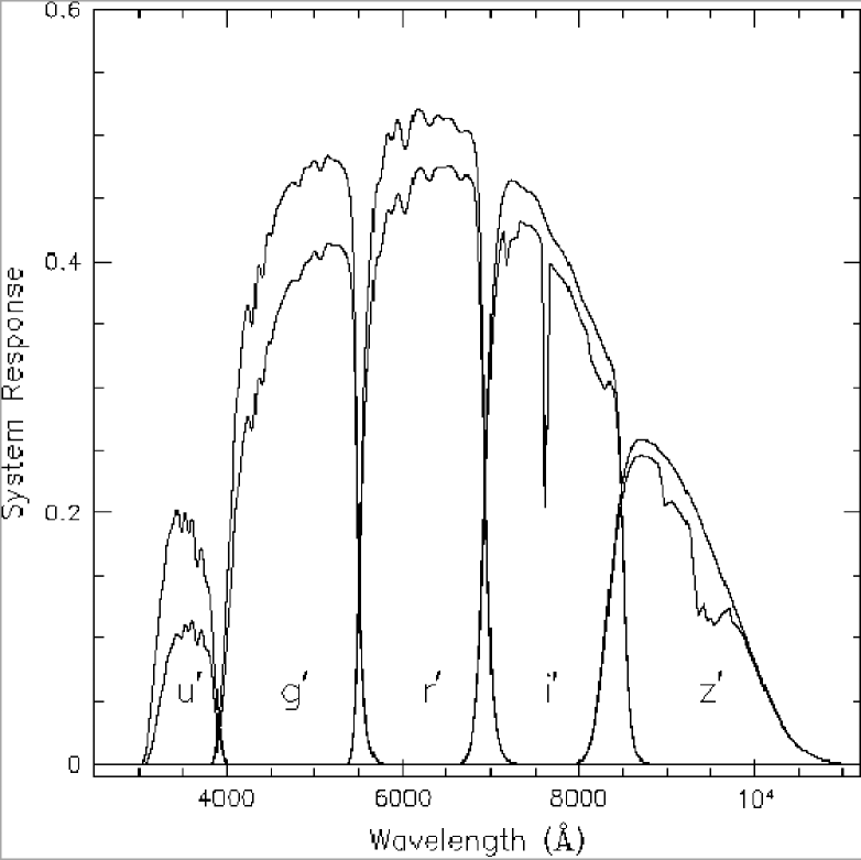
Figure 1: Response function of the SDSS photometric system. Dashed curves indicate the response function including atmospheric transmission at 1.2 airmass at the altitude of Apache Point Observatory.

The optical photometric data were taken from the SDSS (York et al. 2000 and Stoughton et al. 2002). The SDSS consists of an imaging survey of $\pi$ steradians of the northern sky in the five passbands u, g, r ,i, z, in the entire optical range from the atmospheric ultraviolet cutoff in the blue to the sensitivity limit of silicon in the red (Fig. 1). The survey is carried out using a 2.5 m telescope, an imaging mosaic camera with 30 CCDs, two fiber-fed spectrographs and a 0.5 m telescope for the photometric calibration. The imaging survey is taken in drift-scan mode. The imaging data are processed with a photometric pipeline (PHOTO) specially written for the SDSS data.

4.1 The galaxy sample

In order to study the optical cluster properties, we have created a complete galaxy sample for each cluster, by selecting the galaxies in an area centered on the X-ray source position and with radius of 1.5 deg. We used the selection criteria of Yasuda et al. (2001) to define our galaxy sample from the photometric catalog produced by PHOTO. We have selected only objects flagged with PRIMARY, in order to avoid multiple detections in the overlap between adjacent scan lines in two strips of a stripe and between adjacent frames. Objects with multiple peaks (parent) are divided by the deblender in different components (children); if the objects can not be deblended, they are additionally flagged as NODEBLEND. Only isolated objects, child objects and NODEBLEND flagged objects are used in constructing our galaxy sample. The star-galaxy separation is performed in each band using an empirical technique, based on the difference between the model and the PSF magnitude. An object is classified as galaxy if the model magnitude and the Point Spread Function (PSF) magnitude differ by more than 0.145. This method seems to be robust for $r\leq 21$ mag, which is also the completeness limit of the survey in the Northern galactic cap. Since saturated pixels and diffraction spikes can compromise the model-fitting algorithm, some stars can be misclassified as galaxies. Therefore we have rejected all object with saturated pixels and which are flagged as BRIGHT. Furthermore, we have classified an object as a galaxy only if PHOTO classified it as a galaxy in at least two of the three photometric bands g, r, i. After a visual inspection of a sample of galaxies with $r\leq 16$ mag, Yasuda et al. (2001) concluded that the described selection criteria give a sample completeness of 97%, and the same completeness is found for the sample at $16\leq r\leq 21$ mag after comparison with the Medium Deep Survey catalog (MDS) constructed using WFPC2 parallel images from HST. The major reason of missing real galaxies is the rejection of galaxies blended with saturated stars, while spurious galaxy detections are double stars or shredded galaxies with substructures.

4.2 SDSS Galaxy photometry

Since the galaxies do not have sharp edges or a unique surface brightness profile, it is nontrivial to define a flux for each object. PHOTO calculates a number of different magnitudes for each object: model magnitude, Petrosian magnitudes and PSF magnitudes. The model magnitudes are calculated by fitting de Vaucouleurs and exponential model, convolved with the local PSF, to the two dimensional images of the galaxies in the r band. The total magnitude are determined from the better fitting of the two shape function. Galaxy colors are measured by applying the best fit model of an object in the r band to the others bands, measuring the flux in the same effective aperture. However due to a bug of PHOTO, found during the completion of DR1, the model magnitudes are systematically under-estimated by about 0.2 magnitudes for galaxies brighter then 20th magnitude, and accordingly the measured radii are systematically too large (http://www.sdss.org/DR1/products/catalogs/index.html). This error does not affect the galaxy colors but makes the model magnitude useless for the determination of the galaxy total luminosities.

The Petrosian flux is defined by

$$F_{p}=2\pi\int^{f_{2}r_{P}}_{0}{I(r)dr},$$ (1)

where $I(r)$ is the surface brightness profile of the galaxy, and $r_{P}$ is the Petrosian radius satisfying the equation:

$$f_{1}=\frac{2\pi\int^{1.25r_{P}}_{0.8r_{P}}{\frac{I(r)rdr}{{\pi[(1.25r_{P})^{2}-(0.8r_{P})^{2}]}}}}{2\pi\int^{r_{P}}_{0}{\frac{I(r)rdr}{(\pi r_{p}^{2})}}}.$$ (2)

The Petrosian aperture is set to $2r_{P}$, and it encompasses 99$\%$ of the galaxy total light in case of an exponential profile and 82$\%$ in case of a de Vaucouleurs profile (Blanton et al 2001). The Petrosian ratio $f_{1}$ is set to 0.2; at smaller values PHOTO fails to measure the Petrosian ratio, since the $S/N$ is too low. For faint objects the effect of the seeing on Petrosian magnitude is not negligible. As the galaxy size becomes comparable to the seeing disk, the fraction of light measured by the Petrosian quantities approaches the fraction for a PSF, about $95\%$, in which case the flux is reduced for a galaxy with an exponential profile and increased for a galaxy with a de Vaucouleurs profile (Strauss et al. 2002). Thus the Petrosian magnitudes are the best measure of the total light for bright galaxies, but fail to be a good measure for faint objects. In the data analysis of this paper we used the Petrosian magnitudes for galaxies brighter then 20 mag and the psf magnitudes for objects fainter than 20 mag.

5 Optical Luminosity from SDSS data

5.1 Background subtraction

The total optical luminosity of a cluster has to be calculated after the subtraction of the foreground and background galaxy contamination. Since we have used only photometric data from the SDSS galaxy catalog, we have no direct information on the cluster galaxy memberships. There are two different approaches to overcome this problem. Since galaxy clusters show a very well define red sequence in the color magnitude diagram, a galaxy color cut could be use to define the cluster membership (Gladders et al. 2000). On the other hand the background subtraction can be based on the number counts of the projected field galaxies outside the cluster. We chose the latter approach since the former method may introduce a bias against bluer cluster members observed to have varying fractions due to the Butcher-Oemler effect.

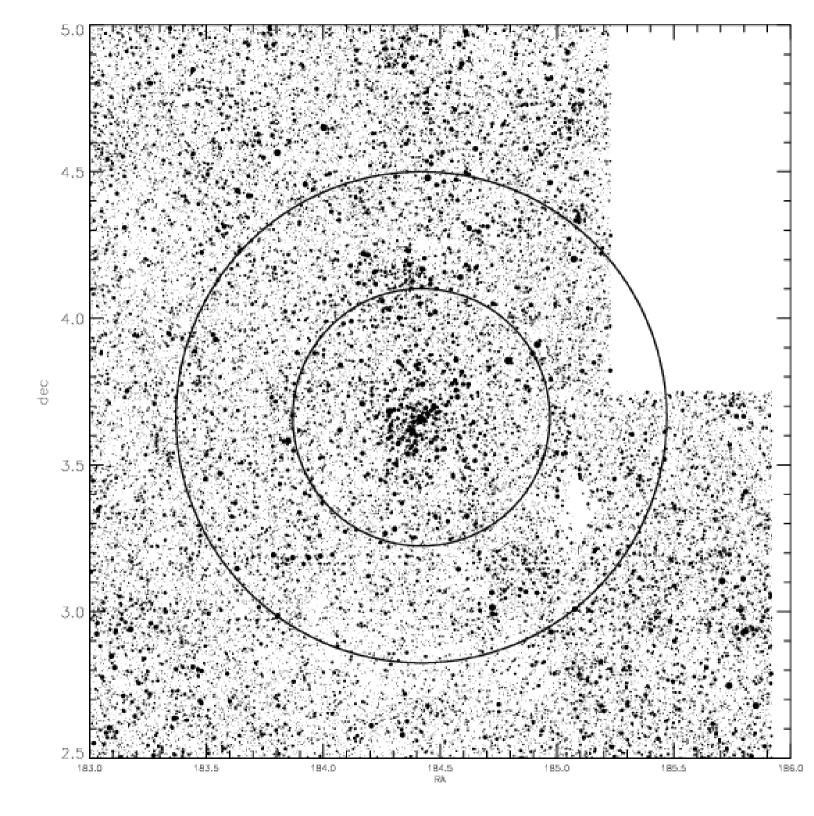
Figure 2: The plot shows a cluster region with the local background. The dots represent the galaxies in the sample. The biggest dots correspond to the brightest galaxies in apparent r magnitude. The local background number counts have been calculated inside the annulus with inner radius equal to $r_{200}+0.2$ deg and a width of $0.5$ degree. The regions with voids due to lack of data or close clusters have to be discarded in the background estimation.

We have considered two different approaches to the statistical subtraction of the galaxy background. First we have calculated a local background. The $M_{200}-L_{X}$ relation of Reiprich et al. 2002 was used to compute the $r_{200}$ radius (where the cluster mass density is 200 times the critical cosmic mass density), as a pragmatic approximation of the virial radius. Then, we defined an annulus centered on the cluster X-ray center, with an inner radius equal to $r_{200}+0.2$ deg and a width of $0.5$ degree (Fig. 2). In this way the galaxy background has been estimated well outside the cluster but still locally. The annulus has been then divided in 20 sectors ( analogous to the approach in Böhringer et al. 2001) and those featuring a larger than $3\sigma$ deviation from the median galaxy density are discarded from the further calculation. In this way other clusters close to the target or voids are not included in the background correction. We have computed the galaxies number counts $N_{bg}^{l}(m)dm$ per bin of magnitude (with a bin width of 0.5 mag) and per squared degree in the remaining area of the annulus. The statistical source of error in this approach is the Poissonian uncertainty of the counts, given by $\sqrt{(N_{bg}^{l}(m))}$.

As a second method we have derived a global background correction. The galaxy number counts $N_{bg}^{g}(m)dm$ was derived from the mean of the magnitude number counts determined in five different SDSS sky regions, each with an area of 30 $\rm{deg^{2}}$ (Fig.3). The source of uncertainty in this second case is systematic and originates the presence of large-scale clustering within the galaxy sample, while the Poissonian error of the galaxy counts is small due to the large area involved. We have estimated this error as the standard deviation of the mean global number counts, $\sigma_{bg}^{g}(m)$, in the comparison of the five areas. In order to take into account this systematic source of error also for the the local background , we have estimated the background number counts error as $\sigma_{bg}(m)=max(\sqrt{(N_{bg}^{l}(m))},\sigma_{bg}^{g}(m))$ (Lumdsen et al. 1997) for all the derived quantities.

After the background subtraction we found that the signal to noise in the u band was too low to be useful, and performed our analysis on the 4 remaining Sloan photometric bands g,r,i,z.

5.2 Luminosity Function

For each cluster and in all photometric bands we have assumed that the distribution function of galaxies in magnitude can be described by the Schechter Luminosity function (LF):

$$\phi(m)dm=0.4\leavevmode\nobreak\ ln(10)\leavevmode\nobreak\ N_{clu}\leavevmode\nobreak\ \phi^{*}\leavevmode\nobreak\ 10^{-0.4\leavevmode\nobreak\ (m-m^{*})\leavevmode\nobreak\ (\alpha-1)}\leavevmode\nobreak\ exp(-10^{-0.4\leavevmode\nobreak\ (m-m^{*})})\leavevmode\nobreak\ dm.$$ (3)

In the equation $N_{clu}$ is the number of cluster galaxies and was computed as the difference between the total number of galaxies in the cluster region and the expected number of interlopers, estimated from the local (global) background galaxy density. $\phi^{*}$ is the normalization of the Schechter Luminosity function, given by the inverse of the integral of the LF over the considered magnitude range. To determine the remaining parameters $M^{*}$ and $\alpha$ we fitted the Schechter LF to the data with a Maximum Likelihood Method (MLM, Sarazin 1980). Since we have no information about the cluster membership, we have considered the observed galaxy magnitude distribution in the cluster region as the sum of the Schechter Luminosity function ($\phi(m)$) plus a background contribution ($b(m)$):

$$\Phi(m)=\frac{\phi(m)+b(m)}{N_{tot}}.$$ (4)

$\Phi(m)$ is normalized to unity when integrated over the considered range of magnitudes.

In order to perform a ML analysis, the background contribution has to be specified at any magnitude. To estimate the $b(m)$, one can try to fit the background number counts by a model. While the behavior of the $N(m)-m$ relation is well know at the bright end (in the $logN(m)-logm$ is a line with slope 0.6, Fig.3) , it is not well understood at the faint end (Yasuda et al. 2001, Lumdsen et al. 1997). Therefore instead of using a specific functional form, we simply have used a spline to interpolate the background galaxy number counts and estimated $b(m)$ at any magnitude.

The probability that the assumed distribution gives a galaxy at the magnitudes $m_{k}$ is thus $\Phi(m_{k})$. Therefore, if the observed galaxies are statistically independent, the combined probability that the assumed distribution gives the observed galaxies at the magnitude $m_{k}$ (with $k=1,n$) is:

$$L=\prod^{n}_{\kappa=1}\Phi(m_{k})$$ (5)

The best-fit parameters are those that maximize the likelihood L. In practice we have minimized the log-likelihood -2ln(L). This minimization was performed with the CERN’s software package MINUIT. We used the variable metric method MIGRAD (Flechter 1970) for the convergence at the minimum and the MINOS routine to estimate the error parameters in case of non linearities. We also have placed constraints on the values of $m^{*}$ and $\alpha$ that the fitting routine can accept, to avoid being trapped in a false minimum ($M*$ in the range between -18 and -26 mag and $\alpha$ between 0 and -2.5, Lumdsen et al. 1997). Fig. 4 gives an example of the LF derived with MLM in each of the Sloan photometric bands for a cluster. Figures 5 and 6 show the comparison between the fit parameters calculated with different backgrounds $b(m)$ (local and global). Fig. 7 shows the correlation between the fit parameters $M^{*}$ and $\alpha$.

The great advantage of the MLM is that the method does not require the data to be binned and does not depend on the bin size, but uses all the available information . On the other hand, the MLM provides no information about the goodness of the fit. Therefore, we have performed a statistical test. Since the routine procedure uses a unbinned set of data to perform the fit, in principle the Kolmogorov Smirnov test should be applicable to our case. Nevertheless since the KS probability is not easy to interpret, we have applied a $\chi^{2}$ test, by comparing the background subtracted magnitude number counts of the cluster with the Schechter luminosity function fitted to the data. Figure 8 shows the distribution of the reduced $\chi^{2}$ in the cluster sample. Almost 90% of the fitted LFs are a good fit to the data having a reduced $\chi^{2}$ $\leq 1$.

5.3 The total luminosity

In order to calculate the total cluster luminosity, we have calculated first the absolute magnitude

$$M=m-25-5log_{10}(D_{L}/1Mpc)-A-K(z)$$ (6)

where $D_{L}$ is the luminosity distance, A is the Galactic extinction and $K(z)$ is the K-correction. We deredden the Petrosian and model magnitudes of galaxies using the Galactic map of Schlegel et al. (1998) in each photometric band. We used the K-correction supplied by Fukugita, Shimasaku, $\&$ Ichikawa (1995) for elliptical galaxies, assuming that the main population of our clusters are the old elliptical galaxies at the cluster redshift. The transformation from absolute magnitudes to absolute luminosity in units of solar luminosities is performed by using the solar absolute magnitude obtained from the color transformation equation from the Johnson-Morgan-Cousins system to the SDSS system of Fukugita et al. (1996). We have calculated the optical luminosity of each cluster with two different methods. First, we have estimated $L$ by using the (background corrected) magnitude number counts of the cluster galaxies with the following prescription:

$$L=\sum_{i}^{N}{N_{i}(m)l_{i}(m)}+\int_{m_{lim}}^{\infty}{\phi(m)dm}$$ (7)

The sum on right side is performed over all the $N$ magnitude bins with galaxy number $N_{i}(m)$ and mean luminosity $l_{i}(m)$. The integral is an incompleteness correction due to the completeness limit of the galaxy sample at $m_{lim}=21$ mag in the five Sloan photometric bands. $\phi(m)$ is the individual Schechter luminosity function fitted to the galaxy sample of each cluster. The incompleteness correction is of the order of 5-10% in the whole cluster sample, as showed in the Fig. 9. This means that the galaxies below the magnitude limit do not give a significant contribution to the total optical luminosity. Therefore the most important source of error is due to the contribution of the background galaxy number counts. The uncertainty in each bin of magnitude is given by the Poissonian error of the bin counts ($\sqrt{N^{i}_{tot}(m)}$, with $i=1,...,N$) and the background subtraction in each magnitude bin ($\sigma_{bg}^{i}(m)$, with $i=1,...,N$, see previous section for the definition). Since the galaxy counts in the bins are independent, the error in the luminosity is given by:

$$\Delta L=(\sum_{i}^{N}{(N^{i}_{tot}(m)+\sigma_{bg}^{i}(m)^{2})})^{\frac{1}{2}}.$$ (8)

Fig. 10 shows the comparison between the luminosity calculated from the local background corrected and global background corrected magnitude number counts. The difference between both methods is much smaller than the statistical error.

In the second case we have taken advantage of the individual fitted luminosity function. If MIGRAD has converged successfully to the minimum, we calculate the total luminosity as

$$L=L^{*}N_{clu}\phi^{*}\Gamma(2+\alpha)$$ (9)

where $L^{*}$ and $\alpha$ are the fit parameters estimated from the data and $N_{clu}$ is the total number of cluster galaxies. There are different sources of errors in this calculation. The major source of error comes from the background which affects both the number of cluster galaxies $N_{clu}$ and the result of the fitting procedure. A second kind of error is due to the uncertainty of the fit parameters. Since all these errors are not independent, we can not treat their contributions separately. Therefore the luminosity errors were calculated by varying the fit parameter values, $M^{*}$ and $\alpha$, along their 68% confidence level error ellipse and using the upper and lower bound of the quoted background number counts ($b(m)$) ranges. The statistical luminosity error range was then defined between the minimum and maximum luminosity. With this method we can take into account statistical and systematic errors due to the background and their effects on the fit parameters as well. Note that a simple error propagation applied to the equation (9) would underestimate the error in the luminosity, since it would not take into account the error of the galaxy background.

Fig. 11 shows the comparison of the two optical luminosities (fit-based and count-based), which are consistent within the errors. For 70% of the clusters in the sample the count-based luminosity is systematically brighter than the the fit-based one, as showed in the Fig. 12. In the former case, indeed, the method includes in the calculation of $L_{op}$ the Bright Cluster Galaxies (BCG) which are usually excluded by the Schechter luminosity function. The error bars in the fit-based luminosity are larger than in the count-based ones. In fact in the former case there are two main sources of error: the uncertainty due to the galaxy background subtraction and the statistical errors in the fit parameters of the luminosity function. In the latter case, Instead, only the subtraction of the galactic background plays a crucial role. The mean error in the fit-based luminosity is around 30%, while it is around 20% with the count-based method.

The great advantages of the count-based optical luminosity is that it can be easily computed, if the cluster $S/N$ is high enough. On the other hand, the fit-based luminosity depends on the success of the fitting procedure. Therefore, it is sensitive not only to the $S/N$ but also to the chosen model and the goodness of the fit. The uncertainty in the count-based method is smaller than in the fit-based method. Moreover, while the count-based method provides the optical luminosity for any system and at any cluster aperture, the number of failures in the fitting procedure is an increasing function of the cluster aperture. In fact the fit-based method fails to fit the data for 15% of the clusters at 0.35 Mpc $\rm{h}_{70}^{-1}$ up to 35% at 2.0 Mpc $\rm{h}_{70}^{-1}$. In consequence, the count-based $L_{op}$ has to be preferred to the fit-based one in the study of the correlation between optical and X-ray properties. The count-based method also reflects what we actually observe.

On the basis of this analysis we can conclude that the behavior of the optical luminosities calculated with different background subtraction is stable for variant approaches and the main source of errors is due to the necessary background subtraction (Fig. 10). Moreover, since the two different methods (count-based and fit-based) give consistent results, our measure of $L_{op}$ seems to be a good estimation of the cluster total optical luminosity.

5.4 The optical structure parameters

In order to study the spatial distribution of galaxies in cluster, we have analysed the projected radial galaxy distributions of each cluster in the sample. The analysis is performed in the g,r i and z bands. As for the luminosity functions, we have used a Maximum Likelihood method to fit a King profile to the data

$$P(r)=\frac{\sigma_{0}}{(1+(\frac{r}{r_{c}})^{2})^{\beta}}+\sigma_{b}.$$ (10)

In equation 10, $\sigma_{0}$ is the central galaxy density, $r_{c}$ the core radius, $\beta$ the profile exponent, and $\sigma_{b}$ the background density. $P(r)$ has to be normalized through:

$$\int_{A}{P(r)d(\pi r^{2})}=N_{tot}$$ (11)

where A is the relevant cluster area and $N_{tot}$ is the total number of galaxies within that area. In agreement with the section 5.2 the the Likelihood is given by:

$$L=\prod^{n}_{\kappa=1}P(r_{\kappa})$$ (12)

where $r_{\kappa}$ is the projected galaxy distance from the X-ray center. We regarded $\beta$, $r_{c}$ and $\sigma_{b}$ as fitting parameters, while $\sigma_{0}$ is a dependent variable and its value is derived from the likelihood normalization, eq. (11). The fitting method worked successfully in average for 95% of the sample in any photometric band; it failed for groups, where the overdensity in comparison to the background density is too low to fit a profile. As shown in the fig. 13, there are no correlations between the parameters, $\sigma_{0}$, $r_{c}$ and $\beta$, with the background density $\sigma_{b}$. Furthermore the histogram of the $\beta$ values in the same figure shows that the mean value of the profile exponent is around 0.8 with a very large dispersion of 0.5 around the peak.

We have estimated from the King profile the physical size of each cluster, $r_{tot}$. We have assumed that this quantity is given by the radial distance from the X-ray center, where the galaxy number density of the cluster becomes $n$ times the error of the background galaxy density ( the cross in the Fig. 14). To search for the best value of $n$, we have estimated the total radius with different values of $n$ ($n=1,...,5$) and calculated the total optical luminosity within that radius; $n$ was then fixed to 3, since the differences in the luminosities calculated within different total radii are smaller than the luminosity uncertainties due to background subtraction.

We assumed that the cluster total optical luminosity in a band is the luminosity calculated within $r_{tot}$ estimated in the given filter. To calculate then the half-light radius , which encircles half of the total cluster luminosity, we have estimated in each band the luminosity of the cluster within 20 radii from the X-ray center to the total radius. We have then interpolated in each filter the 20 luminosities, to find the radius which corresponds to half of the total cluster luminosity.

5.5 The catalog

In the following we present the catalog of the 114 RASS-SDSS galaxy clusters. Tables 1-3 list all the X-ray and optical properties of the sample computed as explained in the previous sections. The examples tables show the results for the first 35 clusters in the sample. The complete tables are given in electronic form.

Table (1) give the X-ray properties of the cluster derived from the ROSAT data. Col. (1) and (2) contain the ROSAT and the alternative cluster name respectively. Col. (3) and (4) contain the equatorial coordinates of the X-ray cluster center used for the regional selection for the epoch J2000 in decimal degrees. Col. (5) contains the heliocentric cluster redshift. Col. (6) presents the flux in the energy band range 0.1-2.4 keV in units of $10^{-11}$ ergs $\rm{s}^{-1}$ $\rm{cm}^{-2}$. Col. (7) gives the corrected flux for a temperature derived from $L_{X}-T$ relation including the K-correction for an assumed cluster temperature of 5 keV. Col. (8) contains the relative 1 $\sigma$ Poissonian error of the count rate, the flux and the luminosity in percent. Col (9) gives the luminosity in the energy range 0.1-2.4 keV in units of $\rm{h}_{70}^{-2}10^{44}$erg $\rm{s}^{-1}$. Col. (10) contains the count rate in units of counts $\rm{s}^{-1}$. Col. (11) gives the outer radius within which the flux and the luminosity are estimated, in units of arc minutes.

Tables (2) provides the optical parameters of the luminosity function and the luminosities of each cluster calculated by using the local galaxy background. Listed are results in the r band. All the quantities are calculated within a fixed cluster aperture of 1.0 Mpc $\rm{h}_{70}^{-1}$. Col. (1) presents the ROSAT name of the cluster. Col. (2) and (3) show the resulting fit parameters of a Schechter luminosity function. $\alpha$ is the slope of the LF, while $M*$ is the magnitude knee of the distribution. Col. (4) gives the galaxy number density within the cluster region selected to perform the fit, in units of $\rm{deg}^{-2}$. Col. (5) shows the reduced $\chi^{2}$ of the fitted luminosity function. Col (6) provides the cluster optical luminosity in units of $10^{12}$ $L_{\odot}$, calculated on the basis of the fitted luminosity function. Col (7) lists the cluster optical luminosity in units of $10^{12}$ $L_{\odot}$, calculated on the base of the cluster magnitude number counts. All the errors in the table are at $68\%$ confidence level. The catalog contains the extended version of this table. Similar tables exist, listing the parameters and the luminosities relative to 22 different cluster apertures: 20 fixed apertures ranging from 0.05 to 4.0 Mpc $\rm{h}_{70}^{-1}$, 2 variable apertures as the core radius and the half-light radius. All the data are provided in each of the 4 Sloan photometric bands g,r,i and z, and for both local and global galaxy background correction.

Table (3) provides the information concerning to the radial distribution of the projected galaxy density in the region of the cluster. Col. (1) presents the ROSAT name of the cluster. Col. (2) gives the cluster central galaxy number density in units of $\rm{deg}^{-2}$ ($\sigma_{0}$ is not a fit parameter, therefore the error is not provided). Col. (3) lists the background galaxy number density around the cluster in units of $\rm{deg}^{-2}$. Col. (4) shows the core radius estimated from the fit, in units of Mpc. Col. (5) provides the cluster total radius, extrapolated from the King profile, in units of Mpc. Col. (6) gives the half-light radius in units of Mpc. All the errors in the table are at $68\%$ confidence level.

The full set of extended tables are available in electronic form.

	Alternative								Count
Name	Name	R.A.	dec	$z$	$F_{X}$	${F_{X}}^{*}$	Error	$L_{X}$	Rate	$R_{out}$
(1)	(2)	(3)	(4)	(5)	(6)	(7)	(8)	(9)	(10)	(11)
RXCJ0041.8-0918	$A0085$	10.4587	-9.3019	0.0520	67.612	67.905	3.0	7.877	3.255	18.0
RXCJ0114.9+0022	$A0168$	18.7350	0.3746	0.0470	8.725	8.484	8.7	0.812	0.423	14.0
RXCJ0119.6+1453	$A0175$	19.9072	14.8931	0.1290	3.124	3.114	29.1	2.237	0.148	9.5
RXCJ0137.2-0912	…	24.3140	-9.2028	0.0390	7.275	7.071	8.4	0.464	0.358	9.5
RXCJ0152.7+0100	$A0267$	28.1762	1.0126	0.2270	4.257	4.276	12.1	9.327	0.209	9.0
RXCJ0736.4+3925	…	114.1040	39.4329	0.1170	8.239	8.239	9.5	4.818	0.369	13.0
RXCJ0747.0+4131	…	116.7537	41.5314	0.0280	3.201	2.431	15.0	0.083	0.147	9.5
RXCJ0753.3+2922	…	118.3291	29.3741	0.0620	6.414	0.062	9.6	1.046	0.302	9.0
RXCJ0758.4+3747	$Ngc2484$	119.6172	37.7888	0.0410	0.605	0.431	32.1	0.032	0.028	7.0
RXCJ0800.9+3602	$A0611$	120.2445	36.0469	0.2880	2.536	2.545	16.9	8.852	0.118	6.0
RXCJ0809.6+3455	…	122.4177	34.9262	0.0800	5.208	5.164	13.2	1.436	0.242	7.5
RXCJ0810.3+4216	…	122.5942	42.2669	0.0640	2.974	2.893	13.8	0.515	0.138	6.0
RXCJ0821.8+0112	…	125.4655	1.2116	0.0820	5.170	5.126	15.5	1.499	0.245	13.5
RXCJ0822.1+4705	$A0646$	125.5417	47.0995	0.1300	7.236	7.236	9.0	5.253	0.346	8.0
RXCJ0824.0+0326	$MS0821.5+0337$	126.0209	3.4383	0.3470	0.297	0.294	78.6	1.577	0.014	2.5
RXCJ0825.4+4707	$A0655$	126.3652	47.1196	0.1260	7.235	7.235	15.1	4.926	0.342	12.0
RXCJ0828.1+4445	…	127.0278	44.7634	0.1450	4.501	4.501	11.2	4.048	0.214	6.0
RXCJ0842.9+3621	$A0697$	130.7401	36.3625	0.2820	5.821	5.858	16.0	19.423	0.281	8.0
RXCJ0845.3+4430	$HGC35$	131.3434	44.5115	0.0540	0.082	0.057	100.0	0.007	0.004	0.5
RXCJ0850.1+3603	$CL0847.2+3617$	132.5499	36.0614	0.3730	2.742	2.75	18.7	15.876	0.134	9.5
RXCJ0913.7+4056	$CL09104+4109$	138.4411	40.9339	0.4420	1.756	1.769	30.1	14.168	0.093	8.5
RXCJ0913.7+4742	$A0757$	138.4446	47.7021	0.0510	6.202	6.022	13.3	0.680	0.315	15.0
RXCJ0917.8+5143	$A0773$	139.4637	51.7223	0.2170	5.961	5.998	9.2	11.853	0.305	9.0
RXCJ0943.0+4700	$A0851$	145.7600	47.0038	0.4060	1.014	1.017	30.8	7.100	0.052	4.5
RXCJ0947.1+5428	…	146.7862	54.4754	0.0460	5.241	15.090	2.6	0.466	0.270	14.0
RXCJ0952.8+5153	…	148.2009	51.8888	0.2140	4.196	4.216	10.6	8.131	0.218	8.0
RXCJ0953.6+0142	…	148.4231	1.7118	0.0980	2.389	2.322	24.3	0.975	0.115	9.5
RXCJ1000.5+4409	…	150.1260	44.1550	0.1540	2.775	2.766	12.6	2.835	0.143	5.0
RXCJ1013.7-0006	…	153.4368	-0.1085	0.0930	3.382	3.353	28.4	1.251	0.162	8.0
RXCJ1017.5+5933	$A0959$	154.3960	59.5577	0.3530	4.079	4.109	11.4	21.151	0.211	13.0
RXCJ1022.5+5006	…	155.6283	50.1030	0.1580	5.389	5.403	9.0	5.773	0.278	8.0
RXCJ1023.6+0411	…	155.9125	4.1873	0.2850	8.562	8.617	8.1	29.215	0.420	7.5
RXCJ1023.6+4908	$A0990$	155.9212	49.1349	0.1440	8.180	8.202	7.3	7.236	0.422	10.0
RXCJ1053.7+5452	…	163.4349	54.8726	0.0750	4.024	3.907	11.5	0.961	0.209	11.0
RXCJ1058.4+5647	…	164.6097	56.7922	0.1360	7.661	7.682	7.0	6.094	0.400	8.5

Table 1: Example of the table containing the X-ray cluster properties of the whole cluster sample. The table show the results for the first 35 cluster in the sample.

Name	$\alpha$	$M*$	$\rho$	$\chi/\nu$	$L_{F}$	$L_{C}$
RXCJ0041.8-0918	$-1.20\pm 0.00$	$0.00\pm 0.00$	0	0.00	$0.000\pm 0.000$	$1.959\pm 0.500$
RXCJ0114.9+0022	$-1.36\pm 0.10$	$-22.17\pm 0.70$	682	1.05	$1.049\pm 0.049$	$1.086\pm 0.393$
RXCJ0119.6+1453	$-1.06\pm 0.20$	$-21.93\pm 0.69$	2775	1.21	$2.588\pm 0.071$	$4.128\pm 1.842$
RXCJ0137.2-0912	$-1.20\pm 0.00$	$0.00\pm 0.00$	0	0.00	$0.000\pm 0.000$	$0.663\pm 0.250$
RXCJ0152.7+0100	$-1.20\pm 0.00$	$0.00\pm 0.00$	0	0.00	$0.000\pm 0.000$	$4.816\pm 1.719$
RXCJ0736.4+3925	$-1.35\pm 0.19$	$-22.30\pm 1.04$	1301	0.67	$1.775\pm 0.078$	$1.575\pm 0.517$
RXCJ0747.0+4131	$-1.20\pm 0.00$	$0.00\pm 0.00$	0	0.00	$0.000\pm 0.000$	$0.156\pm 0.103$
RXCJ0753.3+2922	$-1.58\pm 0.09$	$-22.78\pm 0.96$	1701	1.53	$1.103\pm 0.030$	$1.108\pm 0.444$
RXCJ0758.4+3747	$-1.20\pm 0.00$	$0.00\pm 0.00$	0	0.00	$0.000\pm 0.000$	$0.284\pm 0.190$
RXCJ0800.9+3602	$-0.75\pm 1.06$	$-21.15\pm 1.45$	5733	1.28	$2.429\pm 0.062$	$4.796\pm 3.073$
RXCJ0809.6+3455	$-1.35\pm 0.12$	$-21.50\pm 0.63$	1850	0.56	$1.266\pm 0.023$	$1.247\pm 0.372$
RXCJ0810.3+4216	$-1.56\pm 0.14$	$-22.33\pm 1.27$	975	0.57	$0.593\pm 0.081$	$0.611\pm 0.272$
RXCJ0821.8+0112	$-0.71\pm 0.30$	$-21.42\pm 0.55$	1234	0.68	$1.507\pm 0.026$	$1.577\pm 0.548$
RXCJ0822.1+4705	$-1.20\pm 0.00$	$0.00\pm 0.00$	0	0.00	$0.000\pm 0.000$	$0.913\pm 0.455$
RXCJ0824.0+0326	$-0.77\pm 0.20$	$-20.60\pm 0.37$	3250	0.56	$2.185\pm 0.027$	$2.429\pm 0.677$
RXCJ0825.4+4707	$-1.61\pm 0.19$	$-23.12\pm 1.49$	2641	0.65	$1.743\pm 0.099$	$1.470\pm 0.559$
RXCJ0828.1+4445	$-1.41\pm 0.64$	$-21.33\pm 1.18$	6881	0.28	$3.573\pm 0.148$	$2.385\pm 0.746$
RXCJ0842.9+3621	$0.00\pm 0.57$	$-19.97\pm 0.75$	20	1.06	$0.182\pm 0.022$	$0.238\pm 0.145$
RXCJ0845.3+4430	$-1.20\pm 0.00$	$0.00\pm 0.00$	0	0.00	$0.000\pm 0.000$	$3.972\pm 1.351$
RXCJ0850.1+3603	$-1.20\pm 0.00$	$0.00\pm 0.00$	0	0.00	$0.000\pm 0.000$	$1.655\pm 1.364$
RXCJ0913.7+4056	$-1.24\pm 0.20$	$-21.31\pm 0.89$	308	0.68	$0.474\pm 0.017$	$0.476\pm 0.194$
RXCJ0913.7+4742	$-1.06\pm 0.31$	$-21.35\pm 0.63$	7365	0.72	$3.606\pm 0.075$	$3.795\pm 1.064$
RXCJ0917.8+5143	$-1.20\pm 0.00$	$0.00\pm 0.00$	0	0.00	$0.000\pm 0.000$	$5.492\pm 1.971$
RXCJ0943.0+4700	$-0.01\pm 0.51$	$-19.67\pm 0.47$	54	1.07	$0.681\pm 0.075$	$0.798\pm 0.244$
RXCJ0947.1+5428	$0.00\pm 0.90$	$-20.23\pm 0.87$	1716	0.31	$0.892\pm 0.011$	$1.483\pm 0.696$
RXCJ0952.8+5153	$-2.16\pm 1.45$	$-25.53\pm 0.00$	958	0.72	$0.739\pm 0.000$	$0.904\pm 0.865$
RXCJ0953.6+0142	$-0.69\pm 0.89$	$-21.24\pm 1.67$	411	0.48	$0.505\pm 0.107$	$0.532\pm 0.285$
RXCJ1000.5+4409	$-1.33\pm 0.27$	$-20.91\pm 0.95$	1150	0.95	$0.597\pm 0.018$	$0.617\pm 0.286$
RXCJ1013.7-0006	$-1.20\pm 0.00$	$0.00\pm 0.00$	0	0.00	$0.000\pm 0.000$	$5.320\pm 1.670$
RXCJ1017.5+5933	$-1.24\pm 0.23$	$-21.66\pm 0.75$	3959	0.69	$2.417\pm 0.076$	$2.434\pm 0.717$
RXCJ1022.5+5006	$-0.65\pm 0.72$	$-20.52\pm 0.65$	5544	0.21	$2.265\pm 0.032$	$2.348\pm 0.981$
RXCJ1023.6+0411	$-0.75\pm 0.40$	$-20.58\pm 0.73$	2442	0.60	$1.079\pm 0.036$	$1.309\pm 0.492$
RXCJ1023.6+4908	$-1.31\pm 0.13$	$-21.80\pm 0.65$	1227	1.06	$1.016\pm 0.010$	$1.036\pm 0.358$
RXCJ1053.7+5452	$-1.52\pm 0.21$	$-21.78\pm 1.21$	3964	1.25	$2.397\pm 0.203$	$2.318\pm 0.750$
RXCJ1058.4+5647	$-1.49\pm 0.09$	$-21.98\pm 0.64$	2557	0.63	$1.338\pm 0.011$	$1.338\pm 0.409$

Table 2: Example of the table containing optical properties of the whole cluster sample in the r band. The table show the results for the first 35 clusters in the sample.

Name	$\sigma_{0}$	$\sigma_{b}$	$r_{c}$	$r_{tot}$	$r_{h}$
RXCJ0041.8-0918	5510	$2614\pm 204$	$0.434\pm 0.015$	3.362	$1.229\pm 0.275$
RXCJ0114.9+0022	2299	$4626\pm 52$	$0.195\pm 0.026$	0.940	$0.365\pm 0.061$
RXCJ0119.6+1453	17720	$3796\pm 498$	$0.013\pm 0.003$	1.599	$0.807\pm 0.068$
RXCJ0137.2-0912	5071	$5239\pm 27$	$0.094\pm 0.013$	0.697	$0.300\pm 0.127$
RXCJ0152.7+0100	12846	$4297\pm 607$	$0.044\pm 0.007$	1.344	$0.866\pm 0.103$
RXCJ0736.4+3925	4834	$2083\pm 594$	$0.480\pm 0.022$	2.516	$1.269\pm 0.188$
RXCJ0747.0+4131	0	$0\pm 0$	$0.000\pm 0.000$	0.000	$0.000\pm 0.000$
RXCJ0753.3+2922	5081	$4776\pm 94$	$0.158\pm 0.014$	1.178	$0.413\pm 0.053$
RXCJ0758.4+3747	0	$0\pm 0$	$0.000\pm 0.000$	0.000	$0.000\pm 0.000$
RXCJ0800.9+3602	27566	$4883\pm 382$	$0.015\pm 0.005$	3.044	$1.295\pm 0.581$
RXCJ0809.6+3455	4168	$2428\pm 2908$	$0.688\pm 0.000$	0.000	$0.000\pm 0.000$
RXCJ0810.3+4216	8986	$4433\pm 152$	$0.031\pm 0.009$	0.935	$0.397\pm 0.034$
RXCJ0821.8+0112	8840	$4306\pm 41$	$0.061\pm 0.008$	1.422	$0.553\pm 0.076$
RXCJ0822.1+4705	31953	$5683\pm 153$	$0.007\pm 0.003$	1.183	$0.425\pm 0.107$
RXCJ0824.0+0326	14918	$4046\pm 150$	$0.057\pm 0.006$	2.404	$0.762\pm 0.223$
RXCJ0825.4+4707	44865	$4375\pm 157$	$0.011\pm 0.003$	2.022	$0.506\pm 0.100$
RXCJ0828.1+4445	49497	$3524\pm 396$	$0.007\pm 0.003$	4.451	$2.087\pm 0.548$
RXCJ0842.9+3621	8253	$3760\pm 91$	$0.018\pm 0.007$	0.179	$0.038\pm 0.047$
RXCJ0845.3+4430	25163	$5821\pm 106$	$0.035\pm 0.004$	2.633	$1.477\pm 0.243$
RXCJ0850.1+3603	31130	$2874\pm 402$	$0.005\pm 0.003$	1.479	$1.317\pm 0.063$
RXCJ0913.7+4056	3537	$4338\pm 118$	$0.051\pm 0.014$	0.593	$0.349\pm 0.050$
RXCJ0913.7+4742	42986	$4670\pm 116$	$0.028\pm 0.003$	3.090	$0.602\pm 0.157$
RXCJ0917.8+5143	23067	$3733\pm 227$	$0.025\pm 0.005$	3.137	$0.884\pm 0.183$
RXCJ0943.0+4700	0	$0\pm 0$	$0.000\pm 0.000$	0.000	$0.000\pm 0.000$
RXCJ0947.1+5428	15331	$3898\pm 106$	$0.028\pm 0.006$	1.483	$0.579\pm 0.090$
RXCJ0952.8+5153	3956	$4219\pm 493$	$0.051\pm 0.017$	0.476	$0.270\pm 0.034$
RXCJ0953.6+0142	19978	$3484\pm 85$	$0.017\pm 0.004$	1.065	$0.256\pm 0.063$
RXCJ1000.5+4409	15457	$4581\pm 53$	$0.035\pm 0.006$	1.134	$0.215\pm 0.049$
RXCJ1013.7-0006	44634	$3303\pm 165$	$0.020\pm 0.003$	2.617	$0.883\pm 0.174$
RXCJ1017.5+5933	33538	$4887\pm 121$	$0.020\pm 0.003$	2.166	$0.991\pm 0.300$
RXCJ1022.5+5006	73049	$4563\pm 242$	$0.006\pm 0.003$	2.741	$1.516\pm 0.178$
RXCJ1023.6+0411	14797	$4129\pm 62$	$0.049\pm 0.006$	1.907	$0.337\pm 0.036$
RXCJ1023.6+4908	3003	$5215\pm 53$	$0.175\pm 0.027$	0.712	$0.309\pm 0.066$
RXCJ1053.7+5452	22426	$3428\pm 265$	$0.031\pm 0.005$	2.950	$1.064\pm 0.115$
RXCJ1058.4+5647	4323	$5110\pm 135$	$0.253\pm 0.019$	1.269	$0.450\pm 0.088$

Table 3: Example of the table containing the optical properties of the whole cluster sample in the r band. The table shows the results for the first 35 cluster of the sample.

6 Correlating X-ray and optical properties

For a cluster in which mass traces optical light ($M/L_{opt}$ is constant), the gas is in hyrostatic equilibrium ($T\propto M^{2/3}$), and $L_{X}\propto T^{3}$ (Xue & Wu 2000), we expect the X-ray bolometric luminosity to be related to the optical luminosity as $L_{op}\propto L_{X}^{0.5}$ and to the intracluster medium temperature as $L_{op}\propto T_{X}^{1.5}$.

We have now an optimal data base to test these scaling relations. In a first step we look for those optical parameters which are best suited for a correlation analysis and apply these in a second step to the test of the scaling relations.

In this section we show that tight correlations exist between the total optical cluster luminosity and the X-ray cluster properties as the X-ray luminosity and the intracluster medium temperature.

To search for the best correlation between optical and X-ray properties and to optimally predict for example the X-ray luminosity from the optical appearance, we are interested in an optical characteristic, which shows a minimum scatter in the X-ray/optical correlation. Therefore, we performe a correlation using 4 of the 5 SDSS optical band, $g$, $r$, $i$ and $z$, to find out which filter should be used in the prediction. The $u$ band was not used since the cluster signal to noise in that band is too low to calculate the cluster total luminosity. We used a fixed aperture to calculate the optical luminosities for all the clusters, to make no a priori assumption about the cluster size. Moreover, to check whether the scatter in the correlation depends on the cluster aperture, we did the same analysis several time by using optical luminosities calculated within different radii, ranging from 0.05 to 4 Mpc $\rm{h}_{70}^{-1}$ from the X-ray center. To quantify the $L_{op}-L_{X}$ and the $L_{op}-T_{x}$ relations, a linear regression in log-log space was performed by using two methods for the fitting: a numerical orthogonal distance regression method (ODRPACK) and the bisector method (Akritas $\&$ Bershady 1996). The fits are performed using the form

$$log(L_{op}/L_{\odot})=\alpha log(P_{X})+{\beta}$$ (13)

where $P_{X}$ is the X-ray property, and the errors of each variable are transformed in to log space as $\Delta log(x)=log(e)(x^{+}-x^{-})/(2x)$, where $x^{+}$ and $x^{-}$ denote the upper and lower boundary of the quantity’s error range, respectively. To exclude the outliers in the fitting procedure we apply a $\sigma$ clipping method. After a first fit all the points featuring a larger than $3\sigma$ deviation from the relation, were excluded and the fitting procedure was repeated (see discussion below).

Figs. 15 and 16 show the scatter of the $L_{op}-L_{X}$ and the $L_{op}-T_{x}$ relations, respectively, versus the cluster aperture, used to calculate the optical luminosity. The scatter in the plot is the orthogonal scatter estimated from the best fit given by ODRPACK. In any photometric band the scatter has a clear dependence on the cluster aperture by showing a region of minimum on the very center of the cluster, between 0.2 Mpc $\rm{h}_{70}^{-1}$ and 0.8 Mpc $\rm{h}_{70}^{-1}$, and by increasing at larger radii. The source of the scatter is partially due to the method used to calculate the optical luminosity. Our method is simply based on the overdensity of the cluster with respect of the galaxy background. In fact if the central region in which $L_{op}$ is measured is to small ( 0.05 Mpc $\rm{h}_{70}^{-1}$ in Figs. 15 and 16), the value of the galaxy density is low and the measurement becomes more uncertain. On the other hand, at larger radii the density contrast between cluster and background decreases progressively. Instead, within a cluster aperture between 0.2 Mpc $\rm{h}_{70}^{-1}$ and 0.8 Mpc $\rm{h}_{70}^{-1}$, the optical luminosity of both groups and massive clusters can be easily measured. In fact in both cases the radial aperture is small enough to show an high density contrast and therefore an high cluster signal to noise, and still large to enclose enough galaxies for the luminosity calculation.

After a more accurate analysis, we noted also that the low luminosity systems (both in the optical and in the X-ray band) are the main source of scatter at any cluster aperture. This could be due to different reasons. From the technical point of view the groups have a lower surface density contrast, and this causes problems in calculating the optical luminosity with a method based on the overdensity contrast. Moreover, the low mass systems could have a larger scatter in the optical and X-ray properties.

Furthermore, the galaxy groups could be responsible for the behavior of the scatter shown in fig. 15. In fact at large cluster apertures the galaxy density contrast can be very low for the small systems and still very high for the massive and larger clusters. The large error introduced by the low density contrast in the calculation of the optical luminosity of galaxy groups could be the source of scatter able to explain the increment of the scatter at larger apertures. In order to study in more details the nature of the scatter of our correlation and in order to investigate the role of the less luminous systems, we carried out the analysis explained above with the low mass systems removed. We limited the analysis to the subsample of the X-ray selected REFLEX-NORAS clusters, which occupy the intermediate and high luminosity region. Fig. 17 shows the behavior of the scatter as a function of the cluster aperture in this second analysis. After removing the low mass systems the scatter decreases by about 30% for any aperture (from 0.3 dex to 0.2 dex in the region of minimum scatter and from 0.6 dex in average to 0.4 dex at larger apertures). Nevertheless the behavior of the scatter at increasing aperture is absolutely the same observed in the analysis carried out on the overall RASS-SDSS galaxy cluster sample. This means that groups are responsible for part of the scatter but can not explain the existence of the region of minimum scatter between 0.2 and 0.8 Mpc $\rm{h}_{70}^{-1}$. A possible explanation for the behavior of the scatter at different cluster apertures could be the cluster compactness. As $L_{X}$ depends not only on the cluster mass but also on the compactness of the cluster, also the optical luminosity should reflect somehow the cluster properties, mass and concentration. Thus, there should be an optimal aperture radius within which to measure $L_{op}$. We found that in all photometric bands, the minimum scatter is around 0.5 Mpc $\rm{h}_{70}^{-1}$.

Figg. 18 and 19 show the $L_{op}-L_{X}$ and $L_{op}-T_{x}$ relation respectively, at the radius of minimum scatter, 0.5 Mpc $\rm{h}_{70}^{-1}$, in the z band. In fact the i and the z bands have a slightly smaller scatter than in the other optical bands at any radius. Both plots show, as an outliers, the cluster RXCJ0845.3+4430 , which features a deviation larger than $3\sigma$ from the best fit. The system is a nearby group with a density contrast too low to estimate the optical luminosity reliably. The X-ray luminosity of this system has a 100% error respectively. In the $L_{op}-T_{x}$ there is another outlier: the cluster RXCJ1629.6+4049. This system is not a source of scatter in the $L_{op}-L_{X}$ relation and the error in the X-ray and optical luminosities is 8% and 35% respectively. This can suggests that the optical luminosity is well measured, and it questions the estimate of the temperature. In fact, the X-ray luminosity of RXCJ1629.6+4049 is 2.78$\times 10^{43}$ ergs$\rm{s}^{-1}$, and the temperature, estimated from Horner et al. (2001), is 1 keV, while the $L_{X}-T_{X}$ relation of Xue & Wu, (2000), predicts at least a $T_{X}$ of 4.3 keV at that $L_{X}$.

With the $\sigma$ clipping method those clusters were excluded from the estimation of the best fit. The best fit parameters of the orthogonal and bisector methods, in the i and z photometric bands, are shown in the Table 4 and 5 for the $L_{op}-L_{X}$ relation for the ROSAT X-ray luminosity and the bolometric X-ray luminosity, respectively. Table 6 shows the same results for the $L_{op}-T_{x}$ relation. Table 7 provides the results for the $L_{op}-L_{X}$ relation in i and z band for the subsample of X-ray selected REFLEX-NORAS clusters. The tables show also the estimated orthogonal scatter and the estimated scatter in both the variables. The best fit in the z band for the $L_{op}-L_{X}$ and the $L_{op}-T_{x}$ relations at the radius of minimum scatter for all the RASS-SDSS galaxy cluster sample are respectively:

$$L_{op}/L_{\odot}=10^{11.79\pm 0.02}L_{X}(ROSAT)^{0.45\pm 0.03}$$ (14)

$$L_{op}/L_{\odot}=10^{11.75\pm 0.02}L_{X}(Bol)^{0.38\pm 0.02}$$ (15)

$$L_{op}/L_{\odot}=10^{11.42\pm 0.06}T_{X}^{1.12\pm 0.08}$$ (16)

The value of the exponent in the power law for the $L_{opt}-L_{X}(Bol)$ relation, is around 0.38 in the region of minimum, as indicated in table 4. The values are not consistent within the errors with the value of 0.5 predicted under the assumption of hydrostatic equilibrium and constant mass to light ratio. The same conclusion can be derived for the $L_{opt}-T_{X}$ relation and from the $L_{op}-L_{X}$ for the subsample of X-ray selected REFLEX-NORAS clusters. A simple reason of the disagreement could be due to the assumption of a constant mass to light ratio. In fact, Girardi et al. (2002) analysed in detail the mass to light ratio in the B band of a sample of 294 clusters and groups , finding $M/L\propto L^{0.33\pm 0.03}$. The same results was found by Lin et al. (2003) in the K band. Thus if we consider this dependence of $M/L$ from the optical luminosity with the assumptions of hydrostatic equilibrium, the new expected relation between the optical luminosity and the X-ray luminosity and temperature are $L_{op}\propto L_{X}^{0.4}$ and $L_{op}\propto T_{X}^{1.25}$, respectively, which are in good agreement with our results.

The scatter in the $L_{op}-L_{x}$ relation for the aperture with the best correlation ( 0.5 Mpc $\rm{h}_{70}^{-1}$), in the $L_{op}$ variable is 0.20, and the scatter in the $L_{X}$ variable is 0.22 in the correlations obtained in i and the z bands as shown in the Table 4. Therefore, by calculating the total cluster luminosity in the central part of the system, one can use the $i$ or $z$ band to predict the X-ray luminosity from the optical data with a mean error of $60\%$. In the same way the optical luminosity can be derived from $L_{X}$ with the same uncertainty. As indicated in the table 7 the uncertainty in the prediction of the two variables decreases to less than 40% if the correlation is limited to the REFLEX-NORAS cluster subsample. Table 6 shows that analogous results are obtained for the $L_{op}-T_{x}$ relation.

Since the observational uncertainties in the optical and in the X-ray luminosity are about 20%, the scatters of 60% of the overall sample in both relations and of 40% in the the REFLEX-NORAS cluster subsample for the $L_{op}-L_{x}$ relation should be intrinsic.

$L_{op}-L_{X}(ROSAT)$ relation in the I band
Orthogonal method						Bisector method
$r$	$\alpha$	$\beta$	$\sigma$	$\sigma_{L_{X}}$	$\sigma_{L_{op}}$	$\alpha$	$\beta$	$\sigma$	$\sigma_{L_{X}}$	$\sigma_{L_{op}}$
0.2	$0.50\pm 0.04$	$11.41\pm 0.03$	0.43	0.32	0.30	$0.32\pm 0.01$	1$1.44\pm 0.03$	0.36	0.23	0.28
0.3	$0.46\pm 0.03$	$11.70\pm 0.02$	0.31	0.23	0.21	$0.36\pm 0.01$	1$1.71\pm 0.02$	0.29	0.18	0.23
0.5	$0.47\pm 0.03$	$11.83\pm 0.02$	0.30	0.22	0.20	$0.38\pm 0.01$	1$1.85\pm 0.02$	0.27	0.18	0.20
0.7	$0.56\pm 0.03$	$11.94\pm 0.03$	0.36	0.26	0.25	$0.47\pm 0.01$	1$1.96\pm 0.02$	0.32	0.22	0.24
0.8	$0.61\pm 0.04$	$11.99\pm 0.03$	0.40	0.29	0.28	$0.51\pm 0.01$	1$2.01\pm 0.03$	0.36	0.24	0.26
1.0	$0.65\pm 0.04$	$12.05\pm 0.03$	0.44	0.31	0.31	$0.54\pm 0.01$	1$2.07\pm 0.03$	0.39	0.27	0.28

$L_{op}-L_{X}(ROSAT)$ relation in the Z band
Orthogonal method						Bisector method
$r$	$\alpha$	$\beta$	$\sigma$	$\sigma_{L_{X}}$	$\sigma_{L_{op}}$	$\alpha$	$\beta$	$\sigma$	$\sigma_{L_{X}}$	$\sigma_{L_{op}}$
0.2	$0.50\pm 0.04$	$11.50\pm 0.03$	0.43	0.31	0.31	$0.31\pm 0.01$	$11.54\pm 0.03$	0.35	0.23	0.26
0.3	$0.45\pm 0.03$	$11.79\pm 0.02$	0.31	0.23	0.21	$0.37\pm 0.01$	$11.80\pm 0.02$	0.29	0.18	0.23
0.5	$0.47\pm 0.03$	$11.92\pm 0.02$	0.30	0.22	0.20	$0.39\pm 0.01$	$11.93\pm 0.02$	0.28	0.18	0.21
0.7	$0.56\pm 0.03$	$12.03\pm 0.03$	0.36	0.26	0.25	$0.47\pm 0.01$	$12.04\pm 0.02$	0.33	0.22	0.24
0.8	$0.60\pm 0.04$	$12.08\pm 0.03$	0.40	0.29	0.27	$0.51\pm 0.01$	$12.10\pm 0.03$	0.36	0.24	0.26
1.0	$0.65\pm 0.04$	$12.14\pm 0.03$	0.44	0.31	0.31	$0.54\pm 0.01$	$12.15\pm 0.03$	0.39	0.27	0.28

Table 4: The table presents the results of the best fit for the i and z band in the region of the minimum scatter, $0.2\leq r\leq 1.0$ Mpc $\rm{h}_{70}^{-1}$ for the $L_{op}-L_{X}(ROSAT)$ relation. We show the results for the two methods applied: the orthogonal distance regression (ODRPACK) and the bisector method, which is the line bisecting the best fit results of the vertical and horizontal minimization. The $\alpha$ and $\beta$ parameters are given for several apertures with the 95% confidence errors. The orthogonal scatter and the scatters in log($L_{X}$(0.1-2.4 keV) and in log($L_{op}$) to the best fit line are given by $\sigma$, $\sigma_{L_{X}}$ and $\sigma_{L_{op}}$ respectively.

$L_{op}-L_{X}(Bolometric)$ relation in the I band
Orthogonal method						Bisector method
$r$	$\alpha$	$\beta$	$\sigma$	$\sigma_{L_{X}}$	$\sigma_{L_{op}}$	$\alpha$	$\beta$	$\sigma$	$\sigma_{L_{X}}$	$\sigma_{L_{op}}$
0.2	$0.38\pm 0.03$	$11.25\pm 0.04$	0.41	0.31	0.27	$0.27\pm 0.01$	$11.31\pm 0.03$	0.37	0.24	0.28
0.3	$0.36\pm 0.02$	$11.54\pm 0.03$	0.31	0.23	0.20	$0.30\pm 0.01$	$11.57\pm 0.02$	0.29	0.18	0.23
0.5	$0.38\pm 0.02$	$11.66\pm 0.03$	0.30	0.22	0.20	$0.32\pm 0.01$	$11.70\pm 0.02$	0.27	0.18	0.21
0.7	$0.38\pm 0.02$	$11.66\pm 0.03$	0.30	0.22	0.20	$0.32\pm 0.01$	$11.70\pm 0.02$	0.27	0.18	0.21
0.8	$0.49\pm 0.03$	$11.77\pm 0.04$	0.41	0.30	0.28	$0.42\pm 0.01$	$11.82\pm 0.03$	0.37	0.25	0.27
1.0	$0.53\pm 0.03$	$11.81\pm 0.04$	0.44	0.32	0.31	$0.45\pm 0.01$	$11.86\pm 0.03$	0.40	0.27	0.29

$L_{op}-L_{X}(Bolometric)$ relation in the Z band
Orthogonal method						Bisector method
$r$	$\alpha$	$\beta$	$\sigma$	$\sigma_{L_{X}}$	$\sigma_{L_{op}}$	$\alpha$	$\beta$	$\sigma$	$\sigma_{L_{X}}$	$\sigma_{L_{op}}$
0.2	$0.38\pm 0.03$	$11.34\pm 0.04$	0.41	0.30	0.28	$0.26\pm 0.01$	$11.42\pm 0.03$	0.35	0.23	0.27
0.3	$0.35\pm 0.02$	$11.63\pm 0.03$	0.30	0.24	0.19	$0.31\pm 0.01$	$11.65\pm 0.02$	0.29	0.18	0.23
0.5	$0.38\pm 0.02$	$11.75\pm 0.03$	0.30	0.23	0.20	$0.32\pm 0.01$	$11.78\pm 0.02$	0.28	0.18	0.21
0.7	$0.38\pm 0.02$	$11.75\pm 0.03$	0.30	0.23	0.20	$0.32\pm 0.01$	$11.78\pm 0.02$	0.28	0.18	0.21
0.8	$0.49\pm 0.03$	$11.86\pm 0.04$	0.40	0.29	0.28	$0.42\pm 0.01$	$11.90\pm 0.03$	0.37	0.25	0.27
1.0	$0.52\pm 0.03$	$11.90\pm 0.04$	0.44	0.32	0.31	$0.44\pm 0.01$	$11.95\pm 0.03$	0.40	0.28	0.29

Table 5: The table presents the results of the best fit for the i and z band in the region of the minimum scatter, $0.2\leq r\leq 1.0$ Mpc $\rm{h}_{70}^{-1}$ for the $L_{op}-L_{X}(Bolometric)$ relation. We show the results for the two methods applied: the orthogonal distance regression (ODRPACK) and the bisector method, which is the line bisecting the best fit results of the vertical and horizontal minimization. The $\alpha$ and $\beta$ parameters are given for several apertures with the 95% confidence errors. The orthogonal scatter and the scatters in log($T_{X}$) and in log($L_{op}$) to the best fit line are given by $\sigma$, $\sigma_{T_{X}}$ and $\sigma_{L_{op}}$ respectively.

$L_{op}-T_{X}$ relation in the I band
Orthogonal method						Bisector method
$r$	$\alpha$	$\beta$	$\sigma$	$\sigma_{T_{X}}$	$\sigma_{L_{op}}$	$\alpha$	$\beta$	$\sigma$	$\sigma_{T_{X}}$	$\sigma_{L_{op}}$
0.2	$0.97\pm 0.17$	$11.05\pm 0.12$	0.53	0.39	0.36	$1.22\pm 0.22$	$10.80\pm 0.16$	0.54	0.39	0.37
0.3	$1.06\pm 0.09$	$11.21\pm 0.06$	0.32	0.27	0.17	$1.17\pm 0.18$	$11.12\pm 0.14$	0.31	0.18	0.25
0.5	$1.11\pm 0.08$	$11.33\pm 0.06$	0.26	0.20	0.16	$1.13\pm 0.10$	$11.30\pm 0.08$	0.25	0.17	0.19
0.7	$1.20\pm 0.11$	$11.43\pm 0.08$	0.30	0.23	0.19	$1.40\pm 0.12$	$11.27\pm 0.09$	0.29	0.20	0.21
0.8	$1.20\pm 0.12$	$11.51\pm 0.09$	0.33	0.26	0.20	$1.51\pm 0.13$	$11.26\pm 0.10$	0.33	0.23	0.24
1.0	$1.21\pm 0.14$	$11.60\pm 0.10$	0.39	0.32	0.23	$1.62\pm 0.16$	$11.26\pm 0.12$	0.39	0.27	0.28

$L_{op}-T_{X}$ relation in the Z band
Orthogonal method						Bisector method
$r$	$\alpha$	$\beta$	$\sigma$	$\sigma_{T_{X}}$	$\sigma_{L_{op}}$	$\alpha$	$\beta$	$\sigma$	$\sigma_{T_{X}}$	$\sigma_{L_{op}}$
0.2	$0.97\pm 0.18$	$11.18\pm 0.13$	0.54	0.37	0.40	$1.16\pm 0.18$	$10.95\pm 0.13$	0.55	0.42	0.35
0.3	$1.06\pm 0.08$	$11.31\pm 0.06$	0.31	0.27	0.16	$1.18\pm 0.19$	$11.20\pm 0.15$	0.31	0.18	0.25
0.5	$1.12\pm 0.08$	$11.42\pm 0.06$	0.25	0.20	0.16	$1.12\pm 0.10$	$11.39\pm 0.08$	0.25	0.16	0.19
0.7	$1.20\pm 0.11$	$11.52\pm 0.08$	0.30	0.24	0.19	$1.40\pm 0.12$	$11.34\pm 0.09$	0.30	0.20	0.23
0.8	$1.21\pm 0.12$	$11.60\pm 0.09$	0.34	0.27	0.20	$1.51\pm 0.13$	$11.34\pm 0.10$	0.33	0.23	0.24
1.0	$1.22\pm 0.14$	$11.68\pm 0.10$	0.39	0.32	0.23	$1.62\pm 0.15$	$11.34\pm 0.11$	0.39	0.27	0.28

Table 6: The table presents the results of the best fit for the i and z band in the region of the minimum scatter, $0.2\leq r\leq 1.0$ Mpc $\rm{h}_{70}^{-1}$. We show the results for the two methods applied: the orthogonal distance regression (ODRPACK) and the bisector method, which is the line bisecting the best fit results of the vertical and horizontal minimization. The $\alpha$ and $\beta$ parameters are given for several apertures with the 95% confidence errors. The orthogonal scatter and the scatters in log($T_{X}$) and in log($L_{op}$) to the best fit line are given by $\sigma$, $\sigma_{T_{X}}$ and $\sigma_{L_{op}}$ respectively.

$L_{op}-L_{X}(ROSAT)$ relation for REFLEX-NORAS clusters only
orthogonal method
i band						z band
$r$	$\alpha$	$\beta$	$\sigma$	$\sigma_{L_{X}}$	$\sigma_{L_{op}}$	$\alpha$	$\beta$	$\sigma$	$\sigma_{L_{X}}$	$\sigma_{L_{op}}$
0.2	$0.28\pm 0.04$	$11.48\pm 0.03$	0.32	0.23	0.22	$0.27\pm 0.04$	$11.57\pm 0.03$	0.31	0.23	0.21
0.3	$0.33\pm 0.03$	$11.74\pm 0.02$	0.23	0.16	0.15	$0.34\pm 0.03$	$11.83\pm 0.02$	0.21	0.16	0.15
0.5	$0.36\pm 0.03$	$11.87\pm 0.02$	0.22	0.16	0.15	$0.36\pm 0.03$	$11.97\pm 0.02$	0.22	0.16	0.14
0.7	$0.36\pm 0.03$	$12.01\pm 0.02$	0.24	0.18	0.16	$0.37\pm 0.03$	$12.11\pm 0.02$	0.24	0.17	0.16
0.8	$0.37\pm 0.03$	$12.08\pm 0.03$	0.27	0.20	0.17	$0.37\pm 0.03$	$12.17\pm 0.02$	0.26	0.20	0.17
1.0	$0.37\pm 0.04$	$12.18\pm 0.03$	0.29	0.23	0.18	$0.37\pm 0.04$	$12.28\pm 0.03$	0.28	0.22	0.18

Table 7: The table presents the results of the best fit for the i and z band in the region of the minimum scatter, $0.2\leq r\leq 1.0$ Mpc $\rm{h}_{70}^{-1}$ for the $L_{op}-L_{X}(ROSAT)$ relation in the subsample of REFLEX and NORAS X-ray selected clusters. We show the results for the orthogonal distance regression (ODRPACK) method. The $\alpha$ and $\beta$ parameters are given for several apertures with the 95% confidence errors. The orthogonal scatter and the scatters in log($L_{X}$(0.1-2.4 keV)) and in log($L_{op}$) to the best fit line are given by $\sigma$, $\sigma_{L_{X}}$ and $\sigma_{L_{op}}$ respectively.

7 Summary and Conclusions

We created a database of clusters of galaxies based on the largest available X-ray and optical surveys: the ROSAT All Sky Survey (RASS) and the Sloan Digital Sky Survey (SDSS). The RASS-SDSS galaxy cluster catalog is the first catalog which combines X-ray and optical data for a large number (114) of galaxy clusters. The systems are X-ray selected, ranging from groups of $10^{12.5}$ $M_{\odot}$ to massive clusters of $10^{15}$ $M_{\odot}$ in a redshift range from 0.002 to 0.45. The X-ray (luminosity in the ROSAT band, bolometric luminosity, redshift, center coordinates) and optical properties (Schechter luminosity function parameters, luminosity, central galaxy density, core, total and half-light radii) are computed in a uniform and accurate way. The catalog contains also temperature and iron abundance for a subsample of 53 clusters from the Asca Cluster Catalog and the Group Sample. The resulting RASS-SDSS galaxy cluster catalog, then, constitutes an important database to study the properties of galaxy clusters and in particular the relation of the galaxy population seen in the optical to the properties of the X-ray luminous ICM.

The first investigations reported have shown a tight correlation between the X-ray and optical properties, when the choice of the measurement aperture for the optical luminosity and the optical wavelength band are optimized. We found that the optical luminosity calculated in the i and in the z band correlates better with the X-ray luminosity and the ICM temperature, in comparison to the other Sloan photometric bands. Thus the red optical bands, which are more sensitive to the light of the old stellar population and therefore to the stellar mass of cluster galaxies, have tight correlations with the X-ray properties of the systems.

Moreover, we found that the scatter in the $L_{op}-L_{X}$ and $L_{op}-T_{X}$ relations can be minimized if the optical luminosity is measured within a cluster aperture between 0.2-0.8 Mpc $\rm{h}_{70}^{-1}$, with an absolute minimum of the scatter at 0.5 Mpc $\rm{h}_{70}^{-1}$. The best aperture in the central part of the cluster for the measurement of the optical luminosity is due to the fact that it is a good compromise to simultaneously assess the total richness and the compactness of the cluster.

Finally by using the relations obtained from the z band, we demonstrated that, given the optical properties of a cluster, we can predict the X-ray luminosity and temperature with an accuracy of 60% and vice versa. By restricting the correlation analysis to the subsample of X-ray detected REFLEX-NORAS clusters, the minimum scatter decreases to less than 40% for the $L_{op}-L_{X}$ relation. Since the observational uncertainties in the optical and in the X-ray luminosity are about 20%, the observed scatters in both relations should be intrinsic.

The resulting logarithmic slope for the $L_{op}-L_{X}$ relation with the minimum scatter is $0.38\pm 0.02$, while the value for the $L_{op}-T_{X}$ relation is $1.12\pm 0.08$. Both results are not consistent with the assumption of hydrostatic equilibrium and a constant M/L. If we assume that M/L depends on the luminosity with the power law $M/L\propto L^{0.3}$ (Girardi et al. 2002), our results are in very good agreement with the expected values under the assumption of hydrostatic equilibrium.

The analysis carried out in this paper on the correlation between X-ray and optical apparence of galaxy clusters is completely empirical. In principle, the best way to proceed in this kind of study is to measure the optical luminosity within the physical size of the cluster, like the virial radius. Without optical spectroscopic data or accurate temperature measurements, the cluster virial radius can be calculated by assuming a theoretical model relating the optical luminosity to the cluster mass. At this stage of the work, we preferred to tackle the cluster X-ray-optical connection with the empirical method explained in the paper, in order to have model-independent results. On the other hand, not taking into account the different cluster sizes could have affected both the slope and the scatter of the given relations (eq. 14, 15 and 16). Therefore, for a better understanding of the important connection between the X-ray and optical apparence of galaxy clusters, the optical luminosity has to be calculated within the physical size of the cluster. This work is in progress and will be published in the second paper of this series about the RASS-SDSS galaxy cluster sample. The next step will be the study of the fundamental plane of galaxy clusters. Through this kind of analysis we will find out if the observed scatter in the correlations between the optical and X-ray properties depends on another parameter related to the cluster compactness. Moreover, because of the link between the galaxy cluster fundamental plane and the M/L parameter, we will connect directly the slope of two relations to the behavior of M/L.

Funding for the creation and distribution of the SDSS Archive has been provided by the Alfred P. Sloan Foundation, the Participating Institutions, the National Aeronautics and Space Administration, the National Science Foundation, the U.S. Department of Energy, the Japanese Monbukagakusho, and the Max Planck Society. The SDSS Web site is http://www.sdss.org/. The SDSS is managed by the Astrophysical Research Consortium (ARC) for the Participating Institutions. The Participating Institutions are The University of Chicago, Fermilab, the Institute for Advanced Study, the Japan Participation Group, The Johns Hopkins University, Los Alamos National Laboratory, the Max-Planck-Institute for Astronomy (MPIA), the Max-Planck-Institute for Astrophysics (MPA), New Mexico State University, University of Pittsburgh, Princeton University, the United States Naval Observatory, and the University of Washington.

8 References

Abazajian, K., Adelman, J., Agueros, M.,et al. 2003, AJ, 126, 2081 (Data Release One)
Adami, C. et al. 1998, A&A, 336, 63;
Akritas, M., Mazure, A., Katgert, P., et al. 1996, ApJ, 470, 706;
Arnaud, M., Rothenflug, R.; Boulade, O., et al. 1992, A&A, 254, 49;
Bahcall, N. 1977, ApJL, 217, 77;
Bahcall, N. 1981, ApJ, 247, 787;
Bahcall, N., McKay, T. A., Annis, J., et al. 2003, ApJS, 148, 253;
Blanton, M., Blanton, M. R., Dalcanton, J., Eisenstein, D., et al. 2001, AJ, 121, 2358;
Blanton, M.R., Lupton, R.H., Maley, F.M. et al. 2003, AJ, 125, 2276 (Tiling Algorithm)
Böhringer, H., Voges, W.; Huchra, J. P., et al. 2000, ApJS, 129, 435;
Böhringer, H., Schuecker, P., Guzzo, L., et al. 2001, A&A, 369, 826;
Böhringer, H., Collins, C. A., Guzzo, L., et al. 2002, ApJ, 566, 93;
De grandi, S. and Molendi, S. 2002, ApJ, 567, 163;
De Propris, R., Colless, M., Driver, S. P., et al. 2003, MNRAS, 342, 725;
Donahue, M., Mack, J., Scharf, C., et al. 2001, ApJL, 552, 93;
Donahue, M., Scharf, C. A., Mack, J., et al. 2002, ApJ, 569, 689;
Dressler, A., Oemler, A. Jr., Couch, W. J., et al. 1997, ApJ, 490, 577;
Edge, A. C. & Stewart, G. C. 1991, MNRAS, 252, 428;
Eisenstein, D. J., Annis, J., Gunn, J. E., et al. 2001, AJ, 122, 2267;
Fasano, G., Poggianti, B. M., Couch, W. J., et al. 2000, ApJ, 542, 673;
Finoguenov, A., Arnaud, M., David, L. P. 2001, ApJ, 555, 191F;
Finoguenov, A., Reiprich, T. H., B hringer, H. 2001,A&A,368,749;
Flectcher, R. 1970, Comput. J, 13, 317;
Fukugita, M., Shimasaku, K.; Ichikawa, T. 1995, PASJ, 107,945;
Fukugita, M., Ichikawa, T., Gunn, J. E. 1996, AJ, 111, 1748;
Girardi, M., Borgani, S., Giuricin, G., et al. 2000, ApJ, 530, 62;
Girardi, M., Manzato, P., Mezzetti, M., et al. 2002, ApJ, 569, 720;
Gladders, M. and Yee, H. K. C. 2000, AJ, 120, 2148;
Gomez, P., Nichol, R. C., Miller, C. J., et al. 2003, ApJ, 584, 210;
Goto, T., Sekiguchi, M., Nichol, R. C., et al. 2002, AJ, 123, 1807;
Goto, T., Okamura, S., McKay, T. A., et al. 2002, PASP, 123, 1807;
Gunn, J.E., Carr, M.A., Rockosi, C.M., et al 1998, AJ, 116, 3040 (SDSS Camera)
Hogg, D.W., Finkbeiner, D. P., Schlegel, D. J., Gunn, J. E. 2001, AJ, 122, 2129;
Horner, D. 2001, PhD Thesis, University of Maryland;
Ikebe, Y., Reiprich, T. H., Böhringer, H., et al. 2002, A&A, 383, 773;
Isobe, T., Feigelson, E. D., Akritas, M. G., et al. 1990, ApJ, 364, 104;
Kelson, D., van Dokkum, P. G., Franx, M., et al. 1997, ApJ, 478, 13;
Kelson, D., llingworth, G. D., van Dokkum, P. G., Franx, M. 2000, ApJ, 531, 137;
Kim, R., Seung J., Kepner, J. V. 2002, AJ, 123, 20; Kochanek, C. S., Pahre, M. A., Falco, E. E., et al. 2001, ApJ, 560,566;
Lin, Y., Mohr, J. J., Stanford, S. A. 2003, ApJ,591,749;
Lubin, L., Oke, J. B.; Postman, M. 2002, AJ, 124, 1905;
Lumsden, S. L., Collins, C. A., Nichol, R. C.,et al. 1997, MNRAS, 290, 119;
Lupton, R. H., Gunn, J. E., Szalay, A. S. 1999, AJ, 118, 1406;
Lupton, R., Gunn, J. E., Ivezić, Z., et al. 2001, in ASP Conf. Ser. 238, Astronomical Data Analysis Software and Systems X, ed. F. R. Harnden, Jr., F. A. Primini, and H. E. Payne (San Francisco: Astr. Soc. Pac.), p. 269 (astro-ph/0101420);
Markevitch, M. 1998, ApJ, 504, 27;
Mulchaey, J.S., Davis, D. S., Mushotzky, R. F.; Burstein, D. 2003,ApJSS, 145, 39;
Pier, J.R., Munn, J.A., Hindsley, R.B., et al. 2003, AJ, 125, 1559 (Astrometry)
Poggianti, B. et al., Bridges, T.J., Komiyama, Y., 2003, astro-ph/0309449;
Postman, M., Lubin, L. M., Oke, J. B. 1998, AJ, 116, 560;
Reiprich, T.H. and Böringher H. 2002, ApJ, 567, 716.
Retzlaff, J. 2001,XXIst Moriond Astrophysics Meeting, March 10-17, 2001 Savoie, France. Edited by D.M. Neumann J.T.T. Van.
Rosati, P., Borgani S., Norman, C. 2002, ARAA, 40, 539;
Sarazin, C. 1980, ApJ, 236, 75;
Schlegel, D., Finkbeiner, D. P., Davis, M. 1998, ApJ, 500, 525;
Shimasaku, K., Fukugita, M., Doi, M., et al. 2001, AJ, 122, 1238;
Smith, J.A., Tucker, D.L., Kent, S.M., et al. 2002, AJ, 123, 2121;
Stoughton, C., Lupton, R.H., Bernardi, M., et al. 2002, AJ, 123, 485;
Strateva, I., Ivezić, Z., Knapp, G. R., et al. 2001, AJ, 122, 1861;
Strauss, M. A., M.A., Weinberg, D.H., Lupton, R.H. et al. 2002, AJ, 124, 1810;
Van Dokkum, S., Franx, M., Fabricant, D., et al. 2000, ApJ, 541, 95V;
Voges, W., Aschenbach, B., Boller, Th., et al. 1999, A&A, 349, 389;
Xue, Y. & Wu, X. 2000, ApJ, 538, 65;
Yasuda, N., Fukugita, M. Narayanan, V. K. et al. 2001, AJ, 122, 1104;
Yee, YH. K. C. and Ellingson, E. 2003, ApJ, 585, 215;
York, D. G., Adelman, J., Anderson, J.E., et al. 2000, AJ, 120, 1579;
Ziegler, B. &Bender, R. 1997, MNRAS, 291, 527;

Figure 3: Global background number counts as a function of magnitude in the $r$ band. The error bars include the contribution of large scale structure. The line shows the counts-magnitude relation expected for a homogeneous galaxy distribution in a universe with Euclidean geometry: $N(r)=A_{r}10^{0.6(r-16)}$. The value of $A_{r}=5.99\pm 0.52(0.5mag)^{-1}deg^{-2}$ is the results of the fit in Yasuda et al. 2001 for $12\leq r\leq 17$.

Figure 4: Example of the individual fitted luminosity function of a cluster in 4 Sloan photometric bands. The value of the fitted parameters are indicated in each panel.

Figure 5: Comparison of the $\alpha$ parameter (slope) of the individual Schechter luminosity functions. $\alpha_{L}$ is calculated by using the local background correction, while $\alpha_{G}$ is the result of the global background correction. The different background subtractions give consistent results. The error bars in the plot are at 68% confidence level.

Figure 6: Comparison of the $M*$ parameter (knee) of the individual Schechter luminosity functions. $M*_{L}$ is calculated by using the local background correction, while $M*_{G}$ is the result of the global background correction. As in the case of the slope, the different background subtractions give consistent results. The error bars in the plot are at 68% confidence level.

Figure 7: Fit parameters of the individual Schechter luminosity functions in the r band. The fitting procedure is performed by using the local background magnitude number counts. The parameters show a slight correlation. The error bars in the plot are at 68% confidence level.

Figure 8: Distribution of the reduced $\chi^{2}$ of the individual Schechter luminosity functions. Since the MLM allows us to perform a fit without binning the data but does not give information about the goodness of the fit, we have performed the fitting procedure with MLM and checked the goodness of our fitted luminosity functions with a $\chi^{2}$ test. All the cluster are well represented by the individual fitted luminosity function.

Figure 9: The plot shows the correction for incompleteness to the total optical luminosity. The completeness magnitude limit is 21 mag in each Sloan photometric band. The correction is of the order of 5% for 50% of the cluster in the sample, while it is less than 10% for 85% of the sample. The trend in the plot is due to a selection effect, since the most distant cluster are also the most luminous ones.

Figure 10: Comparison of the cluster optical luminosities calculated from the cluster magnitude number counts with different background corrections. $L_{L}$ is calculated with the local background subtraction, while $L_{G}$ with the global one. The different corrections do not affect the cluster luminosity estimation. The error bars in the plot are at 68% confidence level.

Figure 11: Comparison of the cluster luminosities determined with count-based and fit-based method. The error bars in the plot are at 68% confidence level.

Figure 12: Comparison of the cluster luminosities count-based and fit-based. The plot shows the ratio of the two luminosities (count-based and fit-based) versus the count-based one. For 70% of the sample the ratio $L_{fit-based}/L_{count-based}$ is less the 1.1, indicating that fit-based luminosity is systematically less bright the count-based one. The reason is due to the Bright Cluster Galaxies (BCG): they are included in the computation of the count-based luminosity but not in the estimation of the fit-based one.

Figure 13: The four panels show the behavior of the fit parameters in the King profile fit procedure. The first three panels show that there is no correlation between the parameters, while the bottom right panel presents the histogram of the exponent $\beta$ of the King profile.

Figure 14: The physical total size (the cross) of each cluster is estimated as the radius where the galaxy number density within the cluster becomes 3 times the error in the statistical background galaxy number density (the dashed line).

Figure 15: Orthogonal scatter to the best fit of the $L_{opt}-L_{X}$ relation obtained with the orthogonal method, as a function of the cluster aperture. The scatter shows a minimum in the region $0.2\leq r\leq 0.8$Mpc $\rm{h}_{70}^{-1}$. In the plot different symbols are related to the different photometric bands in which $L_{op}$ is calculated: squares for the g band, triangles for the r band, hexagons for i and filled circles for the z band. The i and z bands show clearly the smallest scatter at any aperture.

Figure 16: Orthogonal scatter to the best fit of the $L_{opt}-T_{X}$ relation obtained with the orthogonal method, as a function of the cluster aperture. The scatter shows a minimum in the region $0.2\leq r\leq 0.8$ Mpc $\rm{h}_{70}^{-1}$. In the plot different symbols are related to the different photometric bands in which $L_{op}$ is calculated: squares for the g band, triangles for the r band, hexagons for i and filled circles for the z band. The i and z bands show clearly the smallest scatter at any aperture.

Figure 17: Orthogonal scatter to the best fit of the $L_{opt}-L_{X}$ relation obtained with the orthogonal method, as a function of the cluster aperture for the subsample of $REFLEX-NORAS$ clusters. The scatter shows again a minimum in the region $0.2\leq r\leq 0.8$Mpc $\rm{h}_{70}^{-1}$. In the plot different symbols are related to the different photometric bands in which $L_{op}$ is calculated: squares for the g band, triangles for the r band, hexagons for i and filled circles for the z band. The i and z bands show clearly the smallest scatter at any aperture.

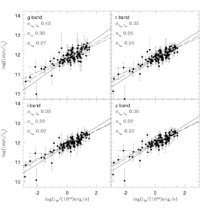
Figure 18: Correlation between optical luminosities and X-ray luminosities. The fit is performed with a linear regression in the $log(L_{opt})-log(L_{X})$ space for each of the 4 optical bands. The solid and the dashed lines are the results of the orthogonal and bisector method respectively over the all RASS-SDSS galaxy cluster sample. The dot-dashed line is the best fit result of the orthogonal method applied to the subsample of strictly X-ray selected REFLEX-NORAS clusters. The error bars are at the 68% confidence level in both the variables.

Figure 19: Correlation between optical luminosities and ICM temperature. The fit is performed with a linear regression in the $log(L_{opt}-log(T_{X}))$ space for each of the 4 optical bands. The solid and the dashed lines are the results of the orthogonal and bisector method respectively. The error bars are at the 68% confidence level in both the variables.