Anisotropies in the Cosmic Microwave Background

Abstract

The linear anisotropies in the temperature of the cosmic microwave background (CMB) radiation and its polarization provide a clean picture of fluctuations in the universe some $370\,\mathrm{kyr}$ after the big bang. Simple physics connects these fluctuations with those present in the ultra-high-energy universe, and this makes the CMB anisotropies a powerful tool for constraining the fundamental physics that was responsible for the generation of structure. Late-time effects also leave their mark, making the CMB temperature and polarization useful probes of dark energy and the astrophysics of reionization. In this review we discuss the simple physics that processes primordial perturbations into the linear temperature and polarization anisotropies. We also describe the role of the CMB in constraining cosmological parameters, and review some of the highlights of the science extracted from recent observations and the implications of this for fundamental physics.

1 Introduction

The cosmic microwave background (CMB) radiation has played an essential role in shaping our current understanding of the large-scale properties of the universe. The discovery of this radiation in 1965 by Penzias and Wilson adc:pw65 , and its subsequent interpretation as the relic radiation from a hot, dense phase of the universe adc:dicke65 put the hot big bang model on a firm observational footing. The prediction of angular variations in the temperature of the radiation, due to the propagation of photons through an inhomogeneous universe, followed shortly after adc:sw67 , but it was not until 1992 that these were finally detected by the Differential Microwave Radiometers (DMR) experiment on the Cosmic Background Explorer (COBE) satellite adc:smoot92 . The fractional temperature anisotropies are at the level of $10^{-5}$, consistent with structure formation in cold dark matter (CDM) models adc:peebles82 ; adc:bond84 , but much smaller than earlier predictions for baryon-dominated universes adc:sw67 ; adc:peebles70 . Another experiment on COBE, the Far InfraRed Absolute Spectrophotometer (FIRAS), spectacularly confirmed the black-body spectrum of the CMB and determined the (isotropic) temperature to be 2.725 K adc:mather94 ; adc:mather99 .

In the period since COBE, many experiments have mapped the CMB anisotropies on a range of angular scales from degrees to arcminutes (see adc:bond03 for a recent review), culminating in the first-year release of all-sky data from the Wilkinson Microwave Anisotropy Probe (WMAP) satellite in February 2003 adc:bennett03 . The observed modulation in the amplitude of the anisotropies with angular scale is fully consistent with predictions based on coherent, acoustic oscillations adc:peebles70 , derived from gravitational instability of initially adiabatic density perturbations in a universe with nearly-flat spatial sections. The amplitude and scale of these acoustic features has allowed many of the key cosmological parameters to be determined with unprecedented precision adc:spergel03 , and a strong concordance with other cosmological probes has emerged.

In this review we describe the essential physics of the temperature anisotropies of the CMB, and its recently-detected polarization adc:kovac02 , and discuss how these are used to constrain cosmological models. For reviews that are similar in spirit, but from the pre-WMAP era see e.g. adc:hu02 ; adc:hu03 . We begin in Sect. 2 with the fundamentals of CMB physics, presenting the kinetic theory of the CMB in an inhomogeneous universe, and the various physical mechanisms that process initial fluctuations in the distribution of matter and spacetime geometry into temperature anisotropies. Section 3 discusses the effect of cosmological parameters on the power spectrum of the temperature anisotropies, and the limits to parameter determination from the CMB alone. The physics of CMB polarization is reviewed in Sect. 4, and the additional information that polarization brings over temperature anisotropies alone is considered. Finally, in Sect. 5 we describe some of the scientific highlights that have emerged from recent CMB observations, including the detection of CMB polarization, implications for inflation, and the direct signature of dark-energy through correlations between the large-scale anisotropies and tracers of the mass distribution in the local universe. Throughout, we illustrate our discussion with computations based on $\varLambda$CDM cosmologies, with baryon density $\varOmega_{\mathrm{b}}h^{2}=0.023$ and cold dark matter density $\varOmega_{\mathrm{c}}h^{2}=0.111$. For flat models we take the dark-energy density parameter to be $\varOmega_{\varLambda}=0.75$ giving a Hubble parameter $H_{0}=73\,\mathrm{km\,s}^{-1}\,\mathrm{Mpc}^{-1}$. We adopt units with $c=1$ throughout, and use a spacetime metric signature $+---$.

2 Fundamentals of CMB Physics

In this section we aim to give a reasonably self-contained review of the essential elements of CMB physics.

2.1 Thermal History and Recombination

The high temperature of the early universe maintained a low equilibrium fraction of neutral atoms, and a correspondingly high number density of free electrons. Coulomb scattering between the ions and electrons kept them in local kinetic equilibrium, and Thomson scattering of photons tended to maintain the isotropy of the CMB in the baryon rest frame. As the universe expanded and cooled, the dominant element hydrogen started to recombine when the temperature fell below $\sim$ 4000 K – a factor of 40 lower than might be anticipated from the 13.6-eV inoization potential of hydrogen, due to the large ratio of the number of photons to baryons. The details of recombination are complicated since the processes that give rise to net recombination occur too slowly to maintain chemical equilibrium between the electrons, protons and atoms during the later stages of recombination adc:peebles68 ; adc:zeldovich69 (see adc:seager00 for recent refinements). The most important quantity for CMB anisotropy formation is the visibility function – the probability that a photon last scattered as a function of time. The visibility function peaks around $\sim 370\,\mathrm{kyr}$ after the big bang, and has a width $\sim 115\,\mathrm{kyr}$, a small fraction of the current age $\sim 13.5\,\mathrm{Gyr}$ adc:spergel03 . After recombination, photons travelled mostly unimpeded through the inhomogeneous universe, imprinting fluctuations in the radiation temperature, the gravitational potentials, and the bulk velocity of the radiation where they last scattered, as the temperature anisotropies that we observe today. A small fraction of CMB photons (current results from CMB polarization measurements adc:kogut03 indicate around 20 per cent; see also Sect. 5.1) underwent further scattering once the universe reionized due to to the ionizing flux from the first non-linear structures.

2.2 Statistics of CMB Anisotropies

The spectrum of the CMB brightness along any direction $\hat{\vec{n}}$ is very nearly thermal with a temperature $T(\hat{\vec{n}})$. The temperature depends only weakly on direction, with fluctuations $\varDelta T(\hat{\vec{n}})$ at the level of $10^{-5}$ of the average temperature $T=2.725$ K. It is convenient to expand the temperature fluctuation in spherical harmonics,

$$\varDelta T(\hat{\vec{n}})/T=\sum_{lm}a_{lm}Y_{lm}(\hat{\vec{n}})\;,$$ (1)

with $a_{lm}^{*}=(-1)^{m}a_{l-m}$ since the temperature is a real field. The sum in (1) runs over $l\geq 1$, but the dipole ($l=1$) is usually removed explicitly when analysing data since it depends linearly on the velocity of the observer. Multipoles at $l$ encode spatial information with characteristic angular scale $\sim\pi/l$.

The statistical properties of the fluctuations in a perturbed cosmology can be expected to respect the symmetries of the background model. In the case of Robertson–Walker models, the rotational symmetry of the background ensures that the multipoles $a_{lm}$ are uncorrelated for different values of $l$ and $m$:

$$\langle a_{lm}a^{*}_{l^{\prime}m^{\prime}}\rangle=C_{l}\delta_{ll^{\prime}}\delta_{mm^{\prime}}\;,$$ (2)

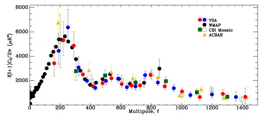
which defines the power spectrum $C_{l}$. The angle brackets in this equation denote the average over an ensemble of realisations of the fluctuations. The simplest models of inflation predict that the fluctuations should also be Gaussian at early times, and this is preserved by linear evolution of the small fluctuations. If Gaussian, the $a_{lm}$s are also independent, and the power spectrum provides the complete statistical description of the temperature anisotropies. For this reason, measuring the anisotropy power spectrum has, so far, been the main goal of observational CMB research. Temperature anisotropies have now been detected up to $l$ of a few thousand; a recent compilation of current data as of February 2004 is given in Fig. 1.

Figure 1: Compilation of CMB anisotropy measurements (as of February 2004) from WMAP (black filled circles), the Very Small Array (VSA adc:dickinson04 ; shaded circles representing two interleaving binning schemes), the Cosmic Background Imager (CBI adc:mason03 ; adc:pearson03 ; open and filled squares for two different binning schemes) and the Arcminute Cosmology Bolometer Array Receiver (ACBAR adc:kuo04 ; triangles). (Figure reproduced, with permission, from adc:dickinson04 .)

The correlation between the temperature anisotropies along two directions evaluates to

$$\langle\varDelta T(\hat{\vec{n}}_{1})\varDelta T(\hat{\vec{n}}_{2})\rangle=T^{2}\sum_{l}\frac{2l+1}{4\pi}C_{l}P_{l}(\cos\theta)\;,$$ (3)

which depends only on the angular separation $\theta$ as required by rotational invariance. Here, $P_{l}(x)$ are the Legendre polynomials. The mean-square temperature anisotropy is

$$\langle\varDelta T^{2}\rangle=T^{2}\sum_{l}\frac{2l+1}{4\pi}C_{l}\approx T^{2}\int\frac{l(l+1)}{2\pi}C_{l}\,\mathrm{d}\ln l\;,$$ (4)

so that the quantity $l(l+1)C_{l}/2\pi$, which is conventionally plotted, is approximately the power per decade in $l$ of the temperature anisotropies.

2.3 Kinetic Theory

The CMB photons can be described by a one-particle distribution function $f(x^{a},p^{a})$ that is a function of the spacetime position $x^{a}$ and four-momentum $p^{a}$ of the photon. It is defined such that the number of photons contained in a proper three-volume element $\mathrm{d}^{3}\vec{x}$ and with three-momentum in $\mathrm{d}^{3}\vec{p}$ is $f\mathrm{d}^{3}\vec{x}\mathrm{d}^{3}\vec{p}$. The phase-space volume element $\mathrm{d}^{3}\vec{x}\mathrm{d}^{3}\vec{p}$ is Lorentz-invariant and is conserved along the photon path through phase space (see, e.g. adc:mtw ). It follows that $f$ is also frame-invariant, and is conserved in the absence of scattering. To calculate the anisotropies in the CMB temperature, we must evolve the photon distribution function in the perturbed universe.

To avoid over-complicating our discussion, we shall only consider spatially-flat models here, and, for the moment, ignore the effects of polarization. For a more complete discussion, including these complications, see e.g. adc:hu98 ; adc:challinor00 . Curvature mostly affects the CMB through the geometrical projection of linear scales at last scattering to angular scales on the sky today, but has a negligible impact on pre-recombination physics and hence much of the discussion in this section. The subject of cosmological perturbation theory is rich in methodology, but, for pedagogical reasons, we adopt here the most straightforward approach which is to work directly with the metric perturbations. This is also the most prevalent in the CMB literature. The 1+3-covariant approach adc:ellis89 is a well-developed alternative that is arguably more physically-transparent than metric-based techniques. It has also been applied extensively in the context of CMB physics adc:challinor00 ; adc:challinor99 ; adc:challinor00b ; adc:maartens99 ; adc:gebbie00a ; adc:gebbie00b . The majority of our discussion will be of scalar perturbations, where all perturbed three-tensors can be derived from the spatial derivatives of scalar functions, although we discuss tensor perturbations briefly in Sect. 2.5.

For scalar perturbations in spatially-flat models we can choose a gauge such that the spacetime metric is adc:ma95

$$\mathrm{d}s^{2}=a^{2}(\eta)[(1+2\psi)\mathrm{d}\eta^{2}-(1-2\phi)\mathrm{d}\vec{x}^{2}]\;,$$ (5)

where $\eta$ is conformal time (related to proper time $t$ by $\mathrm{d}t=a\mathrm{d}\eta$), $a$ is the scale factor in the background model and, now, $\vec{x}$ is comoving position. This gauge, known as the conformal Newtonian or longitudinal gauge, has the property that the congruence of worldlines with constant $\vec{x}$ have zero shear. The two scalar potentials $\phi$ and $\psi$ constitute the scalar perturbation to the metric, with $\phi$ playing a similar role to the Newtonian gravitational potential. In the absence of anisotropic stress, $\phi$ and $\psi$ are equal. We parameterise the photon four-momentum with its energy $\epsilon/a$ and direction $\vec{e}$ (with $\vec{e}^{2}=1$), as seen by an observer at constant $\vec{x}$, so that

$$p^{\mu}=a^{-2}\epsilon[1-\psi,(1+\phi)\vec{e}]\;.$$ (6)

Free photons move on the geodesics of the perturbed metric, $p^{\mu}\nabla_{\mu}p^{\nu}=0$, so the energy and direction evolve as

$$\mathrm{d}\epsilon/\mathrm{d}\eta = -\epsilon\mathrm{d}\psi/\mathrm{d}\eta+\epsilon(\dot{\phi}+\dot{\psi})\;,$$ (7)

$$\mathrm{d}\vec{e}/\mathrm{d}\eta = -\vec{\nabla}_{\perp}(\phi+\psi)\;,$$ (8)

where dots denote $\partial/\partial\eta$ and $\vec{\nabla}_{\perp}$ is the three-gradient projected perpendicular to $\vec{e}$. We see immediately that $\epsilon$ is conserved in the absence of perturbations, so that the energy redshifts in proportion to the scale factor in the background model. The change in direction of the photon due to the projected gradient of the potentials in the perturbed universe gives rise to gravitational lensing (see e.g. adc:bartelmann01 for a review).

The dominant scattering mechanism to affect CMB anisotropies is classical Thomson scattering off free electrons, since around recombination the average photon energy is small compared to the rest mass of the electron. Furthermore, the thermal distribution of electron velocities can be ignored due to the low temperature. The evolution of the photon distribution function in the presence of Thomson scattering is

$$\frac{\mathrm{d}f}{\mathrm{d}\eta} = -a(1+\psi)n_{\mathrm{e}}\sigma_{\mathrm{T}}f+\frac{3}{16\pi}a(1+\psi)n_{\mathrm{e}}\sigma_{\mathrm{T}}\int f(\epsilon,\vec{e}^{\prime})[(1+(\vec{e}\cdot\vec{e}^{\prime})^{2}]\,\mathrm{d}\vec{e}^{\prime}$$ (9)

$$\mbox{}-an_{\mathrm{e}}\sigma_{\mathrm{T}}\vec{e}\cdot\vec{v}_{\mathrm{b}}\epsilon\frac{\partial f}{\partial\epsilon}\;,$$

where $n_{\mathrm{e}}$ is the electron (proper) number density, $\sigma_{\mathrm{T}}$ is the Thomson cross section, and the electron peculiar velocity is $\vec{v}_{\mathrm{b}}=\mathrm{d}\vec{x}/\mathrm{d}\eta$. The derivative on the left of (9) is along the photon path in phase space:

$$\frac{\mathrm{d}f}{\mathrm{d}\eta}=\frac{\partial f}{\partial\eta}+\vec{e}\cdot\vec{\nabla}f+(\dot{\phi}-\vec{e}\cdot\vec{\nabla}\psi)\epsilon\frac{\partial f}{\partial\epsilon}$$ (10)

to first order, where we have used (7) and (8) and the fact that the anisotropies of $f$ are first order. The first term on the right of (9) describes scattering out of the beam, and the second scattering into the beam. The final term arises from the out-scattering of the additional dipole moment in the distribution function seen by the electrons due to the Doppler effect. In the background model $f$ is isotropic and the net scattering term vanishes, so that $f$ is a function of the conserved $\epsilon$ only: $f=\bar{f}(\epsilon)$. Thermal equilibrium ensures that $\bar{f}$ is a Planck function.

The fluctuations in the photon distribution function inherit an energy dependence $\epsilon\partial\bar{f}/\partial\epsilon$ from the source terms in the Boltzmann equation (9). Separating out the background contribution to $f$, and its energy dependence, we can write

$$f(\eta,\vec{x},\epsilon,\vec{e})=\bar{f}(\epsilon)[1-\varTheta(\eta,\vec{x},\vec{e})\mathrm{d}\ln\bar{f}/\mathrm{d}\ln\epsilon],$$ (11)

so that the CMB spectrum is Planckian but with a direction-dependent temperature $\varDelta T/T=\varTheta$. Using the Lorentz invariance of $f$, it is not difficult to show that the quadrupole and higher moments of $\varTheta$ are gauge-invariant. If we now substitute for $f$ in (9), we find the Boltzmann equation for $\varTheta$:

$$\frac{\partial(\varTheta+\psi)}{\partial\eta}+\vec{e}\cdot\vec{\nabla}(\varTheta+\psi) = -an_{\mathrm{e}}\sigma_{\mathrm{T}}\varTheta+\frac{3}{16\pi}an_{\mathrm{e}}\sigma_{\mathrm{T}}\int\varTheta(\vec{e}^{\prime})[(1+(\vec{e}\cdot\vec{e}^{\prime})^{2}]\,\mathrm{d}\vec{e}^{\prime}$$ (12)

$$\mbox{}+an_{\mathrm{e}}\sigma_{\mathrm{T}}\vec{e}\cdot\vec{v}_{\mathrm{b}}+\dot{\phi}+\dot{\psi}\;.$$

The formal solution of this equation is an integral along the line of sight $\hat{\vec{n}}=-\vec{e}$,

$$[\varTheta(\hat{\vec{n}})+\psi]_{R}=\mathrm{e}^{-\tau}[\varTheta(\hat{\vec{n}})+\psi)]_{E}+\int_{E}^{R}\mathrm{e}^{-\tau}S\,\mathrm{d}\eta\;,$$ (13)

where $R$ is the reception event, $E$ is the emission event, and $\tau\equiv\int an_{\mathrm{e}}\sigma_{\mathrm{T}}\,\mathrm{d}\eta$ is the optical depth back from $R$. The source term $S$ is given by the right-hand side of (12), but with $\varTheta$ replaced by $-\psi$ in the first term.

We gain useful insight into the physics of anisotropy formation by approximating the last scattering surface as sharp (which is harmless on large angular scales), and ignoring the quadrupole CMB anisotropy at last scattering. In this case (13) reduces to

$$[\varTheta(\hat{\vec{n}})+\psi]_{R}=\varTheta_{0}|_{E}+\psi|_{E}-\hat{\vec{n}}\cdot\vec{v}_{\mathrm{b}}|_{E}+\int_{E}^{R}(\dot{\psi}+\dot{\phi})\,\mathrm{d}\eta\;,$$ (14)

where $\varTheta_{0}$ is the isotropic part of $\varTheta$, and is proportional to the fluctuation in the photon energy density. The various terms in this equation have a simple physical interpretation. The temperature received along direction $\hat{\vec{n}}$ is the isotropic temperature of the CMB at the last scattering event on the line of sight, $\varTheta_{0}$, corrected for the gravitational redshift due to the difference in potential between $E$ and $R$, and the Doppler shift $\vec{e}\cdot\vec{v}_{\mathrm{b}}|_{E}$ resulting from scattering off moving electrons. Finally, there is an additional gravitational redshift contribution arising from evolution of the gravitational potentials adc:sw67 .

Machinery for an Accurate Calculation

An accurate calculation of the CMB anisotropy on all scales where linear perturbation theory is valid requires a full numerical solution of the Boltzmann equation. The starting point is to expand $\varTheta(\theta,\vec{x},\vec{e})$ in appropriate basis functions. For scalar perturbations, these are the contraction of the (irreducible) trace-free tensor products $e^{\langle i_{1}}\dots e^{i_{l}\rangle}$ (the angle brackets denoting the trace-free part) with trace-free (spatial) tensors derived from derivatives of scalars adc:challinor99 ; adc:gebbie00a ; adc:wilson83 . Fourier expanding the scalar functions, we end up forming contractions between $e^{\langle i_{1}}\dots e^{i_{l}\rangle}$ and $\hat{k}_{\langle i_{1}}\dots\hat{k}_{i_{l}\rangle}$ where $\hat{\vec{k}}$ is the wavevector. These contractions reduce to Legendre polynomials of $\hat{\vec{k}}\cdot\vec{e}$, and so the normal-mode expansion of $\varTheta$ for scalar perturbations takes the form

$$\varTheta(\eta,\vec{x},\vec{e})=\sum_{l\geq 0}\int\frac{\mathrm{d}^{3}\vec{k}}{(2\pi)^{3/2}}(-{\rm i})^{l}\varTheta_{l}(\eta,\vec{k})P_{l}(\hat{\vec{k}}\cdot\vec{e})\mathrm{e}^{{\rm i}\vec{k}\cdot\vec{x}}\;.$$ (15)

It is straightforward to show that the implied azimuthal symmetry about the wavevector is consistent with the Boltzmann equation (12). Inserting the expansion of $\varTheta$ into this equation gives the Boltzmann hierarchy for the moments $\varTheta_{l}$:

$$\dot{\varTheta}_{l}+k\left(\frac{l+1}{2l+3}\varTheta_{l+1}-\frac{l}{2l-1}\varTheta_{l-1}\right) = an_{\mathrm{e}}\sigma_{\mathrm{T}}\left[(\delta_{l0}-1)\varTheta_{l}-\delta_{l1}v_{\mathrm{b}}+\frac{1}{10}\varTheta_{2}\right]$$ (16)

$$\mbox{}+\delta_{l0}\dot{\phi}+\delta_{l1}k\psi\;,$$

where $\vec{v}_{\mathrm{b}}=\int{\rm i}\hat{\vec{k}}v_{\mathrm{b}}(\vec{k})\mathrm{e}^{{\rm i}\vec{k}\cdot\vec{x}}\,\mathrm{d}^{3}\vec{k}/(2\pi)^{3/2}$, and $\phi$ and $\psi$ are the Fourier transforms of the potentials. This system of ordinary differential equations can be integrated directly with the linearised Einstein equations for the metric perturbations, and the fluid equations governing perturbations in the other matter components, as in the publically-available COSMICS code adc:ma95 . Careful treatment of the truncation of the hierarchy is necessary to avoid unphysical reflection of power back down through the moments.

A faster way to solve the Boltzmann equation numerically is to use the line-of-sight solution (13), as in the widely-used CMBFAST code adc:seljak96 and its parallelised derivative CAMB adc:lewis00 . Inserting the expansion (15) gives the integral solution to the hierarchy

$$\varTheta_{l}|_{\eta_{0}} = (2l+1)\int_{0}^{\eta_{0}}\mathrm{d}\eta\,\mathrm{e}^{-\tau}\Big{[}(\dot{\phi}+\dot{\psi})j_{l}(k\varDelta\eta)-\dot{\tau}(\varTheta_{0}+\psi)j_{l}(k\varDelta\eta)$$ (17)

$$\phantom{(2l+1)\int_{0}^{\eta_{0}}\mathrm{d}\eta\,\mathrm{e}^{-\tau}}+\dot{\tau}v_{\mathrm{b}}j_{l}^{\prime}(k\varDelta\eta)-\frac{1}{20}\dot{\tau}\varTheta_{2}(3j_{l}^{\prime\prime}+j_{l})(k\varDelta\eta)\Big{]}\;,$$

where $\varDelta\eta\equiv\eta_{0}-\eta$, $j_{l}$ is a spherical Bessel function, and primes denote derivatives with respect to the argument. Using the integral solution, it is only necessary to evolve the Boltzmann hierarchy to modest $l$ to compute accurately the source terms that appear in the integrand. The integral approach is thus significantly faster than a direct solution of the hierarchy.

The spherical multipoles $a_{lm}$ of the temperature anisotropy can be extracted from (15) as

$$a_{lm}=4\pi{\rm i}^{l}\int\frac{\mathrm{d}^{3}\vec{k}}{(2\pi)^{3/2}}\,\frac{\varTheta_{l}}{2l+1}Y_{lm}^{*}(\hat{\vec{k}})\mathrm{e}^{{\rm i}\vec{k}\cdot\vec{x}}\;.$$ (18)

Statistical homogeneity and isotropy imply that the equal-time correlator

$$\langle\varTheta_{l}(\eta,\vec{k})\varTheta_{l}^{*}(\eta,\vec{k}^{\prime})\rangle=\frac{2\pi^{2}}{k^{3}}\varTheta_{l}^{2}(\eta,k)\delta(\vec{k}-\vec{k}^{\prime})\;,$$ (19)

so forming the correlation $\langle a_{lm}a^{*}_{l^{\prime}m^{\prime}}\rangle$ gives the power spectrum

$$C_{l}=\frac{4\pi}{(2l+1)^{2}}\int\varTheta_{l}^{2}(k)\,\mathrm{d}\ln k\;.$$ (20)

If we consider (pure) perturbation modes characterised by a single independent stochastic amplitude per Fourier mode (such as the comoving curvature for the adiabatic mode; see Sect. 2.4), the power $\varTheta_{l}^{2}(k)$ is proportional to the power spectrum of that amplitude. The spherical Bessel functions in (17) peak sharply at $k\varDelta\eta=l$ for large $l$, so that multipoles $l$ are mainly probing spatial structure with wavenumber $k\sim l/\varDelta\eta$ at last scattering. The oscillatory tails of the Bessel functions mean that some power from a given $k$ does also enter larger scale anisotropies. Physically, this arises from Fourier modes that are not aligned with their wavevector perpendicular to the line of sight. As we discuss in the next section, the tightly-coupled system of photons and baryons undergoes acoustic oscillations prior to recombination on scales inside the sound horizon. For the pure perturbation modes, all modes with a given wavenumber reach the maxima or minima of their oscillation at the same time, irrespective of the direction of $\vec{k}$, and so we expect modulation in the $C_{l}$s on sub-degree scales. The first three of these acoustic peaks have now been measured definitively; see Fig. 1.

2.4 Photon–Baryon Dynamics

Prior to recombination, the mean free path of CMB photons is $\sim 4.9\times 10^{4}(\varOmega_{\mathrm{b}}h^{2})^{-1}(1+z)^{-2}$ Mpc. On comoving scales below this length the photons and baryons behave as a tightly-coupled fluid, with the CMB almost isotropic in the baryon frame. In this limit, only the $l=0$ and $l=1$ moments of the distribution function are significant.

The stress-energy tensor of the photons is given in terms of the distribution function by

$$T^{\mu\nu}=a^{-2}\int f(\eta,\vec{x},\epsilon,\vec{e})p^{\mu}p^{\nu}\epsilon\,\mathrm{d}\epsilon\mathrm{d}\vec{e}\;,$$ (21)

so that the Fourier modes of the fractional over-density of the photons are $\delta_{\gamma}=4\varTheta_{0}$ and the photon (bulk) velocity $v_{\gamma}=-\varTheta_{1}$. The anisotropic stress is proportional to $\varTheta_{2}$. In terms of these variables, the first two moment equations of the Boltzmann hierarchy become

$$\dot{\delta}_{\gamma}-\frac{4}{3}kv_{\gamma}-4\dot{\phi} = 0\;,$$ (22)

$$\dot{v}_{\gamma}+\frac{1}{4}k\delta_{\gamma}-\frac{2}{5}k\varTheta_{2}+k\psi = \dot{\tau}(v_{\gamma}-v_{\mathrm{b}})\;.$$ (23)

Here, the derivative of the optical depth $\dot{\tau}=-an_{\mathrm{e}}\sigma_{\mathrm{T}}$ (and so is negative). The momentum exchange between the photons and baryons due to the drag term in (23) gives rise to a similar term in the Euler equation for the baryons:

$$\dot{v}_{\mathrm{b}}+\mathcal{H}v_{\mathrm{b}}+k\psi=R^{-1}\dot{\tau}(v_{\mathrm{b}}-v_{\gamma})\;,$$ (24)

where we have ignored baryon pressure. The ratio of the baryon energy density to the photon enthalpy is $R\equiv 3\rho_{\mathrm{b}}/4\rho_{\gamma}$ and is proportional to the scale factor $a$, and $\mathcal{H}\equiv\dot{a}/a$ is the conformal Hubble parameter.

In the tightly-coupled limit $|\dot{\tau}^{-1}|\ll k^{-1}$ and $\mathcal{H}^{-1}$. In this limit, we can treat the ratios of the mean-free path to the wavelength and the Hubble time as small perturbative parameters. Equations (23) and (24) then imply that $v_{\gamma}=v_{\mathrm{b}}$ to first order in the small quantities $k/|\dot{\tau}|$ and $\mathcal{H}/|\dot{\tau}|$. Comparing the continuity equation for the baryons,

$$\dot{\delta}_{\mathrm{b}}-kv_{\mathrm{b}}-3\dot{\phi}=0\;,$$ (25)

with that for the photons, we see that $\dot{\delta}_{\gamma}=4\dot{\delta}_{\mathrm{b}}/3$, so the evolution of the photon–baryon fluid is adiabatic, preserving the local ratio of the number densities of photons to baryons. Combining (23) and (24) to eliminate the scattering terms, and then using $v_{\gamma}=v_{\mathrm{b}}$, we find the evolution of the photon velocity to leading order in tight coupling:

$$\dot{v}_{\gamma}+\frac{R}{1+R}\mathcal{H}v_{\gamma}+\frac{1}{4(1+R)}k\delta_{\gamma}+k\psi=0\;.$$ (26)

The $l>1$ moments of the photon distribution function arise from the balance between isotropisation by scattering and their generation by photons free streaming over a mean free path; these moments are suppressed by factors $(k/|\dot{\tau}|)^{l-1}$. In particular, during tight coupling $\varTheta_{2}\approx(20/27)k\dot{\tau}^{-1}v_{\gamma}$ ignoring polarization. (The factor $20/27$ rises to $8/9$ if we correct for polarization adc:kaiser83 .)

Combining (26) with the photon continuity equation (22) shows that the tightly-coupled dynamics of $\delta_{\gamma}$ is that of a damped, simple-harmonic oscillator driven by gravity adc:hu95a :

$$\ddot{\delta}_{\gamma}+\frac{\mathcal{H}R}{1+R}\dot{\delta}_{\gamma}+\frac{1}{3(1+R)}k^{2}\delta_{\gamma}=4\ddot{\phi}+\frac{4\mathcal{H}R}{1+R}\dot{\phi}-\frac{4}{3}k^{2}\psi\;.$$ (27)

The damping term arises from the redshifting of the baryon momentum in an expanding universe, while photon pressure provides the restoring force which is weakly suppressed by the additional inertia of the baryons. The WKB solutions to the homogeneous equation are

$$\delta_{\gamma}=(1+R)^{-1/4}\cos kr_{\mathrm{s}}\;,\phantom{xx}\mathrm{and}\phantom{xx}\delta_{\gamma}=(1+R)^{-1/4}\cos kr_{\mathrm{s}}\;,$$ (28)

where the sound horizon $r_{\mathrm{s}}\equiv\int_{0}^{\eta}\mathrm{d}\eta^{\prime}/\sqrt{3(1+R)}$. Note also that for static potentials, and ignoring the variation of $R$ with time, the mid-point of the oscillation of $\delta_{\gamma}$ is shifted to $-4(1+R)\psi$. The dependence of this shift on the baryon density produces a baryon-dependent modulation of the height of the acoustic peak in the temperature anisotropy power spectrum; see Section 3.

The driving term in (27) depends on the evolution of the gravitational potentials. If we ignore anisotropic stress, $\phi$ and $\psi$ are equal, and their Fourier modes evolve as

$$\ddot{\phi}+3\mathcal{H}\left(1+\frac{\dot{p}}{\dot{\rho}}\right)\dot{\phi}+\left[2\dot{\mathcal{H}}+\left(1+3\frac{\dot{p}}{\dot{\rho}}\right)\mathcal{H}^{2}\right]\phi + \frac{\dot{p}}{\dot{\rho}}k^{2}\phi$$ (29)

$$= \frac{1}{2}\kappa a^{2}\left(\delta p-\frac{\dot{p}}{\dot{\rho}}\delta\rho\right)$$

in a flat universe, which follows from the perturbed Einstein field equations. Here, $\rho$ and $p$ are the total density and pressure in the background model, $\delta\rho$ and $\delta p$ are the Fourier modes of their perturbations, and $\kappa\equiv 8\pi G$. The source term is gauge-invariant; it vanishes for mixtures of barotropic fluids [$p_{i}=p_{i}(\rho_{i})$] with $\delta\rho_{i}/(\rho_{i}+p_{i})$ the same for all components. For adiabatic perturbations, this latter condition holds initially and is preserved on super-Hubble scales. It is also preserved in the tightly-coupled photon–baryon fluid as we saw above. For adiabatic perturbations, the potential is constant on scales larger than the sound horizon when $p/\rho$ is constant, but decays during transitions in the equation of state, such as from matter to radiation domination. Above the sound horizon in flat models, it can be shown that the quantity

$$\mathcal{R}\equiv-\phi-2\frac{\mathcal{H}\dot{\phi}+\mathcal{H}^{2}}{\kappa a^{2}(\rho+p)}$$ (30)

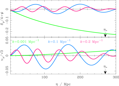
is conserved even through such transitions. The perturbation to the intrinsic curvature of comoving hypersurfaces (i.e. those perpendicular to the the four-velocity of observers who see no momentum density) is given in terms of $\mathcal{R}$ as $4(k^{2}/a^{2})\mathcal{R}$. Using the constancy of $\mathcal{R}$ on large scales, the potential falls by a factor of $9/10$ during the transition from radiation to matter domination. The evolution of the potential is illustrated in Fig. 2 in a flat $\varLambda$CDM model with parameters given in Sect. 1. The potential oscillates inside the sound horizon during radiation domination since the photons, which are the dominant component at that time, undergo acoustic oscillations on such scales.

Figure 2: Evolution of the potential $\phi$ in adiabatic and CDM-isocurvature models for wavenumbers $k=0.001$, $0.01$ and $0.1\,\mathrm{Mpc}^{-1}$ (top to bottom respectively in matter domination). The conformal time at matter–radiation equality $\eta_{\mathrm{eq}}$ and last scattering $\eta_{*}$ are marked by arrows.

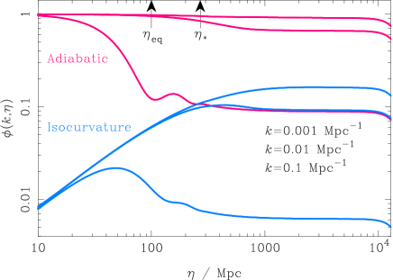
The behaviour of the potentials for isocurvature perturbations is quite different on large scales during radiation domination adc:hu95b , since the source term in (29) is then significant. In isocurvature fluctuations, the initial perturbations in the energy densities of the various components compensate each other in such a way that the comoving curvature $\mathcal{R}=0$. Figure 2 shows the evolution of CDM-isocurvature modes, in which there is initially a large fractional perturbation in the dark matter density, with a small compensating fractional perturbation in the radiation. (The full set of possibilities for regular isocurvature modes are discussed in adc:bucher00 .) On large scales in radiation domination the potential grows as $a$, the scale factor.

Adiabatic Fluctuations

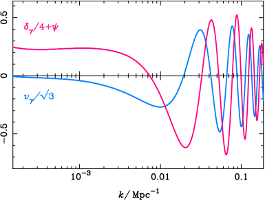
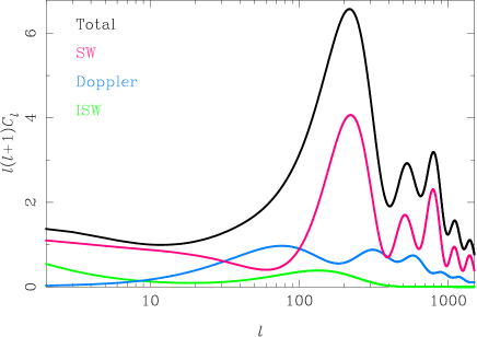
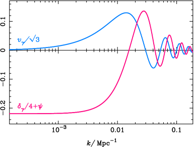
For adiabatic fluctuations, the photons are initially perturbed by $\delta_{\gamma}(0)=-2\psi(0)=4\mathcal{R}(0)/3$, i.e. they are over-dense in potential wells, and their velocity vanishes $v_{\gamma}(0)=0$. If we consider super-Hubble scales at last scattering, there has been insufficient time for $v_{\gamma}$ to grow by gravitational infall and the action of pressure gradients and it remains small. The photon continuity equation (22) then implies that $\delta_{\gamma}-4\phi$ remains constant, and the decay of $\phi$ through the matter–radiation transition leaves $(\delta_{\gamma}/4+\psi)(\eta_{*})\approx\phi(\eta_{\ast})/3=-3\mathcal{R}(0)/5$ on large scales ($k<3\times 10^{-3}\,\mathrm{Mpc}^{-1}$) at last scattering. The combination $\delta_{\gamma}/4+\psi=\varTheta_{0}+\psi$ is the dominant contribution to the large-scale temperature anisotropies produces at last scattering; see (14). The evolution of the photon density and velocity perturbations for adiabatic initial conditions are show in Fig. 3, along with the scale dependence of the fluctuations at last scattering. The plateau in $(\delta_{\gamma}/4+\psi)(\eta_{*})$ on large scales ensures that a scale-invariant spectrum of curvature perturbations translates into a scale-invariant spectrum of temperature anisotropies, $l(l+1)C_{l}=\mathrm{constant}$, for small $l$.

Figure 3: Evolution of the combination $\delta_{\gamma}/4+\psi$ (top left) and the photon velocity $v_{\gamma}$ (bottom left) which determine the temperature anisotropies produced at last scattering (denoted by the arrow at $\eta_{*}$). Three modes are shown with wavenumbers $k=0.001$, $0.1$ and $0.2\,\mathrm{Mpc}^{-1}$, and the initial conditions are adiabatic. The fluctuations at the time of last scattering are shown as a function of linear scale in the right-hand plot.

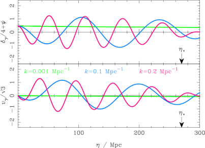
On scales below the sound horizon at last scattering, the photon–baryon fluid has had time to undergo acoustic oscillation. The form of the photon initial condition, and the observation that the driving term in (27) mimics the cosine WKB solution of the homogeneous equation (see Fig. 2), set the oscillation mostly in the $\cos kr_{\mathrm{s}}$ mode. The midpoint of the oscillation is roughly at $\delta_{\gamma}/4=-(1+R)\psi$. This behaviour is illustrated in Fig. 3. Modes with $kr_{\mathrm{s}}(\eta_{*})=\pi$ have undergone half an oscillation at last scattering, and are maximally compressed. The large value of $\varTheta_{0}+\psi$ at this particular scale gives rise to the first acoustic peak in Fig. 1, now measured to be at $l=220.1\pm 0.8$ adc:page03 . The subsequent extrema of the acoustic oscillation at $kr_{\mathrm{s}}(\eta_{*})=n\pi$ give rise to the further acoustic peaks. The angular spacing of the peaks is almost constant and is set by the sound horizon at last scattering and the angular diameter distance to last scattering. The acoustic part of the anisotropy spectrum thus encodes a wealth of information on the cosmological parameters; see Sect. 3. The photon velocity $v_{\gamma}$ oscillates as $\sin kr_{\mathrm{s}}$, so the Doppler term in (14) tends to fill in power between the acoustic peaks. The relative phase of the oscillation of the photon velocity has important implications for the polarization properties of the CMB as discussed in Sect. 4. The contributions of the various terms in (14) to the temperature-anisotropy power spectrum are shown in Fig. 4 for adiabatic perturbations.

Figure 4: Contribution of the various terms in (14) to the temperature-anisotropy power spectrum from adiabatic initial conditions. At high $l$, the contributions are (from top to bottom): total power; $\delta_{\gamma}/4+\psi$ (denoted SW for Sachs–Wolfe adc:sw67 ); Doppler effect from $v_{\mathrm{b}}$; and the integrated Sachs–Wolfe effect (ISW) coming from evolution of the potential along the line of sight.

Isocurvature Fluctuations

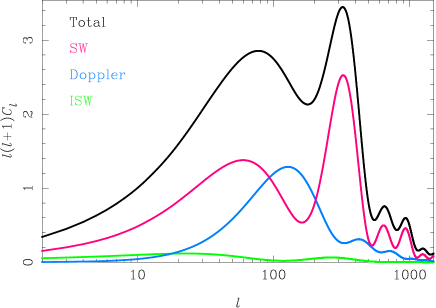
For the CDM-isocurvature mode the photons are initially unperturbed, as is the geometry: $\delta_{\gamma}(0)=0=\phi(0)$ and $v_{\gamma}=0$. On large scales $\delta_{\gamma}/4=\phi$ is preserved, so the growth in $\phi$ during radiation domination is matched by a growth in $\delta_{\gamma}$ and the photons are under-dense in potential wells. It follows that at last scattering $(\delta_{\gamma}/4+\psi)(\eta_{*})\approx 2\phi(\eta_{*})$ for $k<3\times 10^{-3}\,\mathrm{Mpc}^{-1}$. Note that the redshift climbing out of a potential well enhances the intrinsic temperature fluctuation due to the photon under-density there. The evolution of the photon fluctuations for isocurvature initial conditions are shown in Fig. 5.

Figure 5: As Fig. 3 but for CDM-isocurvature initial conditions.

The evolution of the potential for isocurvature modes makes the driving term in (27) mimic the sine solution of the homogeneous equation, and so $\delta_{\gamma}$ follows suit oscillating as $\sin\sim kr_{\mathrm{s}}$ about the equilibrium point $-4(1+R)\psi$. The acoustic peaks are at $kr_{\mathrm{s}}(\eta_{*})\sim n\pi/2$, and the photons are under-dense in the potential wells for the odd-$n$ peaks, while over-dense in the even $n$. The various contributions to the temperature-anisotropy power spectrum for isocurvature initial conditions are shown in Fig. 6. The different peak positions for isocurvature initial conditions allow the CMB to constrain their relative contribution to the total fluctuations. Current constraints are rather dependent on whether one allows for correlations between the adiabatic and isocurvature modes (as are generic in the multi-field inflation models that might have generated the initial conditions), and the extent to which additional cosmological constraints are employed; see adc:bucher04 for a recent analysis allowing for the most general correlations but a single power-law spectrum.

Figure 6: As Fig. 4 but for CDM-isocurvature initial conditions. The initial spectrum of entropy perturbations is scale-invariant.

Beyond Tight-Coupling

On small scales it is necessary to go beyond tight-coupling of the photon–baryon system since the photon diffusion length can become comparable to the wavelength of the fluctuations. Photons that have had sufficient time to diffuse of the order of a wavelength can leak out of over-densities, thus damping the acoustic oscillations and generating anisotropy adc:silk68 . A rough estimate of the comoving scale below which diffusion is important is the square root of the geometric mean of the particle horizon (or conformal age) and the mean-free path of the photons, i.e. $\sqrt{\eta/|\dot{\tau}|}$. Converting this to a comoving wavenumber defines the damping scale

$$k_{\mathrm{D}}^{-2}\sim 0.3(\varOmega_{\mathrm{m}}h^{2})^{-1/2}(\varOmega_{\mathrm{b}}h^{2})^{-1}(a/a_{*})^{5/2}\,\mathrm{Mpc}^{2}$$ (31)

when the scale factor is $a$. Here, $a_{*}$ is the scale factor at last scattering, and the expression is valid well after matter–radiation equality but well before recombination. The effect of diffusion is to damp the photon (and baryon) oscillations exponentially by the time of last scattering on comoving scales smaller than $\sim 3\,\mathrm{Mpc}$. The resulting damping effect on the temperature power spectrum has now been measured by several experiments adc:dickinson04 ; adc:pearson03 ; adc:kuo04 .

To describe diffusion damping more quantitatively, we consider scales that were already sub-Hubble during radiation domination. The gravitational potentials will then have been suppressed during their oscillatory phase when the photons (which are undergoing acoustic oscillations themselves) dominated the energy density, and so we can ignore gravitational effects. Furthermore, the dynamical timescale of the acoustic oscillations is then short compared to the expansion time and we can ignore the effects of expansion. In this limit, the Euler equations for the photons and the baryons can be iterated to give the relative velocity between the photons and baryons to first order in $k/|\dot{\tau}|$:

$$(1+R^{-1})(v_{\gamma}-v_{\mathrm{b}})=\frac{1}{4}k\dot{\tau}^{-1}\delta_{\gamma}\;.$$ (32)

Using momentum conservation for the total photon–baryon system gives

$$\dot{v}_{\gamma}+R\dot{v}_{\mathrm{b}}+\frac{1}{4}k\delta_{\gamma}-\frac{2}{5}k\varTheta_{2}=0\;,$$ (33)

which can be combined with the derivative of (32) to give a new Euler equation for the photons correct to first order in tight coupling:

$$(1+R)\dot{v}_{\gamma}\approx-\frac{1}{4}k\delta_{\gamma}+\frac{R^{2}}{4(1+R)}k\dot{\tau}^{-1}\dot{\delta}_{\gamma}+\frac{16}{45}k^{2}\dot{\tau}^{-1}v_{\gamma}\;.$$ (34)

Here, we have used $\varTheta_{2}\approx 8k\dot{\tau}^{-1}v_{\gamma}/9$ which includes the correction due to polarization. In the limit of perfect coupling, (34) reduces to (26) on small scales. The continuity equation for the photons, $\dot{\delta}_{\gamma}=4kv_{\gamma}/3$ ($+4\dot{\phi}$), shows that the last two terms on the right of (34) are drag terms, and on differentiating gives

$$\ddot{\delta}_{\gamma}-\frac{k^{2}\dot{\tau}^{-1}}{3(1+R)}\left(\frac{16}{15}+\frac{R^{2}}{1+R}\right)\dot{\delta}_{\gamma}+\frac{k^{2}}{3(1+R)}\delta_{\gamma}=0\;.$$ (35)

The WKB solution is

$$\delta_{\gamma}\propto\mathrm{e}^{\pm{\rm i}kr_{\mathrm{s}}}\mathrm{e}^{-k^{2}/k_{\mathrm{D}}^{2}}\;,\quad\mathrm{where}\quad\frac{1}{k_{\mathrm{D}}^{2}}\equiv\frac{1}{6}\int_{0}^{\eta}\frac{|\dot{\tau}^{-1}|}{1+R}\left(\frac{16}{15}+\frac{R^{2}}{1+R}\right)\,\mathrm{d}\eta^{\prime}$$ (36)

is the damping scale.

The finite mean-free path of CMB photons around last scattering has an additional effect on the temperature anisotropies. The visibility function $-\dot{\tau}\mathrm{e}^{\tau}$ has a finite width $\sim 80\,\mathrm{Mpc}$ and so along a given line of sight photons will be last scattered over this interval. Averaging over scattering events will tend to wash out the anisotropy from wavelengths short compared to the width of the visibility function. This effect is described mathematically by integrating the oscillations in the spherical Bessel functions in (17) against the product of the visibility function and the (damped) perturbations.

Boltzmann codes such as CMBFAST adc:seljak96 and CAMB adc:lewis00 use the tight-coupling approximation at early times to avoid the numerical problems associated with integrating the stiff Euler equations in their original forms (23) and (24).

2.5 Other Features of the Temperature-Anisotropy Power Spectrum

We end this section on the fundamentals of the physics of CMB temperature anisotropies by reviewing three additional effects that contribute to the linear anisotropies.

Integrated Sachs–Wolfe Effect

The integrated Sachs–Wolfe (ISW) effect is described by the last term on the right of (14). It is an additional source of anisotropy due to the temporal variation of the gravitational potentials along the line of sight: if a potential well deepens as a CMB photon crosses it then the blueshift due to infall will be smaller than redshift from climbing out of the (now deeper) well. (The combination $\phi+\psi$ has a direct geometric interpretation as the potential for the electric part of the Weyl tensor adc:stewart90 .) The ISW receives contributions from late times as the potentials decay during dark-energy domination, and at early times around last scattering due to the finite time since matter–radiation equality.

The late-time effect contributes mainly on large angular scales since there is little power in the potentials at late times on scales that entered the Hubble radius during radiation domination. The late ISW effect is the only way to probe late-time structure growth (and hence e.g. distinguish between different dark-energy models) with linear CMB anisotropies, but this is hampered by cosmic variance on large angular scales. The late ISW effect produces correlations between the large-scale temperature fluctuations and other tracers of the potential in the local universe, and with the advent of the WMAP data these have now been tentatively detected adc:boughn04 ; adc:nolta03 ; adc:fosalba03 ; see also Sect. 5.

In adiabatic models the early-time ISW effect adds coherently with the contribution $\delta_{\gamma}/4+\psi$ to the anisotropies near the first peak, boosting this peak significantly adc:hu95a ; see Fig. 4. The reason is that the linear scales that contribute here are maximally compressed with $\delta_{\gamma}/4+\psi\sim-\psi/2$ which has the same sign as $\dot{\phi}$ for decaying $\phi$.

Reionization

Once structure formation had proceeded to produce the first sources of ultra-violet photons, the universe began to reionize. The resulting free electron density could then re-scatter CMB photons, and this tended to isotropise the CMB by averaging the anisotropies from many lines of sight at the scattering event. Approximating the bi-modal visibility function as two delta functions, one at last scattering $\eta_{*}$ and one at reionization $\eta_{\mathrm{re}}$, if the optical depth through reionization is $\tau_{\mathrm{re}}$, the temperature fluctuation at $\vec{x}=0$ at $\eta_{0}$ is

$$[\varTheta(\hat{\vec{n}})+\psi]_{\eta_{0}} \approx (1-\mathrm{e}^{-\tau_{\mathrm{re}}})(\varTheta_{0}+\psi-\hat{\vec{n}}\cdot\vec{v}_{\mathrm{b}})[-\hat{\vec{n}}(\eta_{0}-\eta_{\mathrm{re}}),\eta_{\mathrm{re}}]$$ (37)

$$\mbox{}+\mathrm{e}^{-\tau_{\mathrm{re}}}(\varTheta_{0}+\psi-\hat{\vec{n}}\cdot\vec{v}_{\mathrm{b}})[-\hat{\vec{n}}(\eta_{0}-\eta_{*}),\eta_{*}]\;.$$

Here, we have used (13), neglected the ISW effect, and approximated the scattering as isotropic. The first term on the right describes the effect of blending the anisotropies from different lines of sight (to give $\varTheta_{0}$) and the generation of new anisotropies by re-scattering off moving electrons at reionization; the second term is simply the temperature anisotropy that would be observed with no reionization, weighted by the fraction of photons that do not re-scatter. Since $\varTheta_{0}+\psi$ at the re-scattering event is the average of $\varTheta_{0}+\psi-\hat{\vec{n}}^{\prime}\cdot\vec{v}_{\mathrm{b}}$ on the electron’s last scattering surface, on large scales $k(\eta_{\mathrm{re}}-\eta_{*})\ll 1$ it reduces to $\varTheta_{0}+\psi$ at $[-\hat{\vec{n}}(\eta_{0}-\eta_{*}),\eta_{*}]$, while on small scales it vanishes. It follows that for scales that are super-horizon at reionization, the observed temperature anisotropy becomes

$$\varTheta(\hat{\vec{n}})\rightarrow\varTheta(\hat{\vec{n}})-(1-\mathrm{e}^{-\tau_{\mathrm{re}}})\hat{\vec{n}}\cdot\varDelta\vec{v}_{\mathrm{b}}\;,$$ (38)

where $\varDelta\vec{v}_{\mathrm{b}}$ is the difference between the electron velocity at the reionization event and the preceding last scattering event on the line of sight. On such scales the Doppler terms do not contribute significantly and the temperature anisotropy is unchanged. For scales that are sub-horizon at reionization,

$$\varTheta(\hat{\vec{n}})\rightarrow\mathrm{e}^{-\tau_{\mathrm{re}}}\varTheta(\hat{\vec{n}})-(1-\mathrm{e}^{-\tau_{\mathrm{re}}})\hat{\vec{n}}\cdot\vec{v}_{\mathrm{b}}\;,$$ (39)

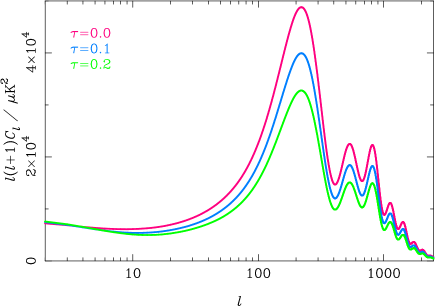
where the Doppler term is evaluated at reionization. In practice, the visibility function is not perfectly sharp at reionization and the integral through the finite re-scattering distance tends to wash out the Doppler term since only plane waves with their wavevectors near the line of sight contribute significantly to $\hat{\vec{n}}\cdot\vec{v}_{\mathrm{b}}$. Figure 7 shows the resulting effect $C_{l}\rightarrow\mathrm{e}^{-2\tau_{\mathrm{re}}}C_{l}$ on the anisotropy power spectrum on small scales. Recent results from WMAP adc:kogut03 suggest an optical depth through reionization $\tau_{\mathrm{re}}\sim 0.17$. Such early reionization cannot have been an abrupt process since the implied redshift $z_{\mathrm{re}}\sim 15$ is at odds with the detection of traces of smoothly-distributed neutral hydrogen at $z\sim 6$ via Gunn-Peterson troughs in the spectra of high-redshift quasars adc:becker01 ; adc:djorgovski01 .

Figure 7: Effect of reionization on the temperature-anisotropy power spectrum. The spectra are (from top to bottom) for no reionization, $\tau_{\mathrm{re}}=0.1$ and $0.2$.

Tensor Modes

Tensor modes, describing gravitational waves, represent the transverse trace-free perturbations to the spatial metric:

$$\mathrm{d}s^{2}=a^{2}(\eta)[\mathrm{d}\eta^{2}-(\delta_{ij}+h_{ij})\mathrm{d}x^{i}\mathrm{d}x^{j}]\;,$$ (40)

with $h_{i}^{i}=0$ and $\partial_{i}h^{i}_{j}=0$. A convenient parameterisation of the photon four-momentum in this case is

$$p^{\mu}=\frac{\epsilon}{a^{2}}\left[1,e^{i}-\frac{1}{2}h^{i}_{j}e^{j}\right]\;,$$ (41)

where $\vec{e}^{2}=1$ and $\epsilon$ is $a$ times the energy of the photon as seen by an observer at constant $\vec{x}$. The components of $\vec{e}$ are the projections of the photon direction for this observer on an orthonormal spatial triad of vectors $a^{-1}(\partial_{i}-h_{i}^{j}\partial_{j}/2)$. In the background $\vec{e}=\mathrm{d}\vec{x}/\mathrm{d}\eta$ and is constant. The evolution of the comoving energy $\epsilon$ in the perturbed universe is

$$\frac{1}{\epsilon}\frac{\mathrm{d}\epsilon}{\mathrm{d}\eta}+\frac{1}{2}\dot{h}_{ij}e^{i}e^{j}=0\;,$$ (42)

and so the Boltzmann equation for $\varTheta(\eta,\vec{x},\vec{e})$ is

$$\frac{\partial\varTheta}{\partial\eta}+\vec{e}\cdot\vec{\nabla}\varTheta = -an_{\mathrm{e}}\sigma_{\mathrm{T}}\varTheta+\frac{3}{16\pi}an_{\mathrm{e}}\sigma_{\mathrm{T}}\int\varTheta(\vec{e}^{\prime})[(1+(\vec{e}\cdot\vec{e}^{\prime})^{2}]\,\mathrm{d}\vec{e}^{\prime}$$ (43)

$$\mbox{}-\frac{1}{2}\dot{h}_{ij}e^{i}e^{j}\;.$$

Neglecting the anisotropic nature of Thomson scattering, the solution of this equation is an integral along the unperturbed line of sight:

$$\varTheta(\hat{\vec{n}})=-\frac{1}{2}\int_{0}^{\eta_{0}}\mathrm{e}^{-\tau}\dot{h}_{ij}\hat{n}^{i}\hat{n}^{j}\,\mathrm{d}\eta\;.$$ (44)

The time derivative $\dot{h}_{ij}$ is the shear induced by the gravitational waves. This quadrupole perturbation to the expansion produces an anisotropic redshifting of the CMB photons and an associated temperature anisotropy.

Figure 8: The temperature-anisotropy power spectrum from scalar perturbations (density perturbations; top) and tensor perturbations (gravity waves; bottom) for a tensor-to-scalar ratio $r=1$.

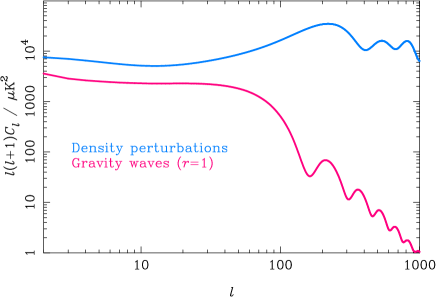
Figure 8 compares the power spectrum due to gravitational waves with that from scalar perturbations for a tensor-to-scalar ratio $r=1$ corresponding to an energy scale of inflation $3.3\times 10^{16}\,\mathrm{GeV}$. The constraints on gravitational waves from temperature anisotropies are not very constraining since their effect is limited to large angular scales where cosmic variance from the dominant scalar perturbations is large. Gravitational waves damp as they oscillate inside the horizon, so the only significant anisotropies are from wavelengths that are super-horizon at last scattering, corresponding to $l\sim 60$. The current 95-per cent upper limit on the tensor-to-scalar ratio is 0.68 adc:dickinson04 . Fortunately, CMB polarization provides an alternative route to detecting the effect of gravitational waves on the CMB which is not limited by cosmic variance adc:seljak97 ; adc:kamionkowski97 ; see also Sect. 4.

3 Cosmological Parameters and the CMB

The simple, linear physics of CMB temperature anisotropies, reviewed in the previous section, means that the CMB depends sensitively on many of the key cosmological parameters. For this reason, CMB observations over the past decade have been a significant driving force in the quest for precision determinations of the cosmological parameters. It is not our intention here to give a detailed description of the constraints that have emerged from such analyses, e.g. adc:bond03 , but rather to provide a brief description of how the key parameters affect the temperature-anisotropy power spectrum. More details can be found in the seminal papers on this subject, e.g. adc:hu95a ; adc:hu95b ; adc:bond94 and references therein.

3.1 Matter and Baryons

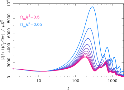
The curvature of the universe and the properties of the dark energy are largely irrelevant for the pre-recombination physics of the acoustic oscillations. Their main contribution is felt geometrically through the angular diameter distance to last scattering, $D_{\mathrm{A}}$, which controls the projection of linear scales there to angular scales on the sky today. In contrast, those parameters that determine the energy content of the universe before recombination, such as the physical densities in (non-relativistic) matter $\varOmega_{\mathrm{m}}h^{2}$, and radiation $\varOmega_{\mathrm{r}}h^{2}$ (determined by the CMB temperature and the physics of neutrinos), play an important role in acoustic physics by determining the expansion rate and hence the behaviour of the perturbations. In addition, the physical density in baryons, $\varOmega_{\mathrm{b}}h^{2}$, affects the acoustic oscillations through baryon inertia and the dependence of the photon mean-free path on the electron density. The effect of variations in the physical densities of the matter and baryon densities on the anisotropy power spectrum is illustrated in Fig. 9 for adiabatic initial conditions.

Figure 9: Dependence of the temperature-anisotropy power spectrum on the physical density in baryons (left) and all non-relativistic matter (right). From top to bottom at the first peak, the baryon densities vary linearly in the range $\varOmega_{\mathrm{b}}h^{2}=0.06$–0.005 (left) and the matter densities in $\varOmega_{\mathrm{m}}h^{2}=0.05$–$0.5$ (right). The initial conditions are adiabatic.

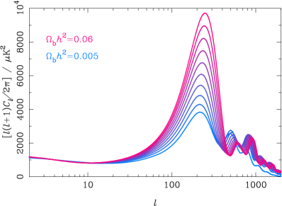
The linear scales at last scattering that have reached extrema of their oscillation are determined by the initial conditions (i.e. adiabatic or isocurvature) and the sound horizon $r_{\mathrm{s}}(\eta_{*})$. Increasing the baryon density holding the total matter density fixed reduces the sound speed while preserving the expansion rate (and moves last scattering to slightly earlier times). The effect is to reduce the sound horizon at last scattering and so the wavelength of those modes that are at extrema of their oscillation, and hence push the acoustic peaks to smaller scales. This effect could be confused with a change in the angular diameter distance $D_{\mathrm{A}}$, but fortunately baryons have another distinguishing effect. Their inertia shifts the zero point of the acoustic oscillations to $\sim-(1+R)\psi$, and enhances the amplitude of the oscillations. In adiabatic models for modes that enter the sound horizon in matter domination, $\delta_{\gamma}/4$ starts out at $-2\psi/3$, and so the amplitude of the oscillation is $-\psi(1+3R)/3$. The combination of these two effects is to enhance the amplitude of $\varTheta_{0}+\psi$ at maximal compression by a factor of $1+6R$ over that at minimal compression. The effect on the power spectrum is to enhance the amplitude of the 1st, 3rd etc. peaks for adiabatic initial conditions, and the 2nd, 4th etc. for isocurvature. Current CMB data gives $\varOmega_{\mathrm{b}}h^{2}=0.023\pm 0.001$ for power-law $\varLambda$CDM models adc:spergel03 , beautifully consistent with determinations from big bang nucleosynthesis. Other effects of baryons are felt in the damping tail of the power spectrum since increasing the baryon density tends to inhibit diffusion giving less damping at a given scale.

The effect of increasing the physical matter density $\varOmega_{\mathrm{m}}h^{2}$ at fixed $\varOmega_{\mathrm{b}}h^{2}$ is also two-fold (see Fig. 9): (i) a shift of the peak positions to larger scales due to the increase in $D_{\mathrm{A}}$; and (ii) a scale-dependent reduction in peak height in adiabatic models. Adiabatic modes that enter the sound horizon during radiation domination see the potentials decay as the photon density rises to reach maximal compression. This decay tends to drive the oscillation, increasing the oscillation amplitude. Raising $\varOmega_{\mathrm{m}}h^{2}$ brings matter–radiation equality to earlier times, and reduces the efficiency of the gravitational driving effect for the low-order peaks. Current CMB data gives $\varOmega_{\mathrm{m}}h^{2}=0.13\pm 0.01$ for adiabatic, power-law $\varLambda$CDM models adc:spergel03 .

3.2 Curvature, Dark Energy and Degeneracies

Figure 10: Dependence of the temperature-anisotropy power spectrum on the curvature $\varOmega_{K}$ (left) and cosmological constant $\varOmega_{\varLambda}$ (right) in adiabatic models. In both cases, the physical densities in baryons and matter were held constant, thus preserving the conditions on the last scattering surface. The curvature varies (left to right) in the range -0.15–0.15 and the cosmological constant in the range 0.9–0.0.

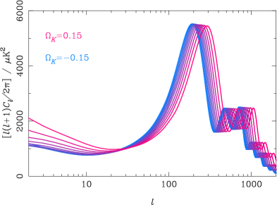
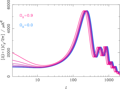
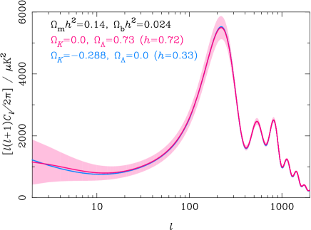
The main effect of curvature and dark energy on the linear CMB anisotropies is through the angular diameter distance and the late-time integrated Sachs–Wolfe effect; see Fig. 10 for the case of adiabatic fluctuations in cosmological-constant models. The ISW contribution is limited to large scales where cosmic variance severely limits the precision of power spectrum estimates. There is an additional small effect due to quantisation of the allowed spatial modes in closed models (e.g. adc:abbott86 ), but this is also confined to large scales (i.e. near the angular projection of the curvature scale). Most of the information that the CMB encodes on curvature and dark energy is thus locked in the angular diameter distance to last scattering, $D_{\mathrm{A}}$.

With the physical densities $\varOmega_{\mathrm{b}}h^{2}$ and $\varOmega_{\mathrm{m}}h^{2}$ fixed by the acoustic part of the anisotropy spectrum, $D_{\mathrm{A}}$ can be considered a function of $\varOmega_{K}$ and the history of the energy density of the dark energy (often modelled through its current density and a constant equation of state). In cosmological constant models $D_{A}$ is particularly sensitive to the curvature: the 95-per cent interval from WMAP alone (with the weak prior $H_{0}>50\,\mathrm{km}\,\mathrm{s}^{-1}\,\mathrm{Mpc}^{-1}$) is $-0.08<\varOmega_{K}<0.02$, so the universe is close to being spatially flat. The fact that the impact of curvature and the properties of the dark energy on the CMB is mainly through a single number $D_{\mathrm{A}}$ leads to a geometrical degeneracy in parameter estimation adc:efstathiou99 , as illustrated in Fig. 11. Fortunately, this is easily broken by including other, complementary cosmological datasets. The constraint on curvature from WMAP improves considerably when supernovae measurements adc:reiss98 ; adc:perlmutter99 , or the measurement of $H_{0}$ from the Hubble Space Telescope Key Project adc:freedman01 are included. Other examples of near-perfect degeneracies for the temperature anisotropies include the addition of gravity waves and a reduction in the amplitude of the initial fluctuations mimicing the effect of reionization. This degeneracy is broken very effectively by the polarization of the CMB.

Figure 11: The geometric degeneracy. A scale-invariant adiabatic $\varLambda$CDM model with $\varOmega_{\mathrm{b}}h^{2}=0.024$, $\varOmega_{\mathrm{m}}h^{2}=0.14$ and $\varOmega_{\varLambda}=0.73$ and $\varOmega_{K}=0$ (close to the WMAP best-fit values adc:spergel03 ) produces an almost identical spectrum to a closed model $\varOmega_{K}=-0.288$ with vanishing cosmological constant. However, the Hubble constants are very different – $h=0.72$ in the flat model and $0.33$ in the closed model – and so the latter is easily ruled out by external constraints. The shaded region shows the $1\sigma$ cosmic variance errors $\varDelta C_{l}/C_{l}=\sqrt{2/(2l+1)}$ on the power spectrum.

4 CMB Polarization

The growth in the mean-free path of the CMB photons during recombination allowed anisotropies to start to develop. Subsequent scattering of the radiation generated (partial) linear polarization from the quadrupole anisotropy. This linear polarization signal is expected to have an r.m.s. $\sim 5\,\mu\mathrm{K}$, and, for scalar perturbations, to peak around multipoles $l\sim 1000$ corresponding to the angle subtended by the mean-free path around last scattering. The detection of CMB polarization was first announced in 2002 by the Degree Angular Scale Interferometer (DASI) team adc:kovac02 ; WMAP has also detected the polarization indirectly through its correlation with the temperature anisotropies adc:kogut03 . A direct measurement of the polarization power from two-years of WMAP data is expected shortly. Polarization is only generated by scattering, and so is a sensitive probe of conditions at recombination. In addition, large-angle polarization was generated by subsequent re-scattering as the universe reionized, providing a unique probe of the ionization history at high redshift.

4.1 Polarization Observables

Polarization is conveniently described in terms of Stokes parameters $I$, $Q$, $U$ and $V$, where $I$ is the total intensity discussed at length in the previous section. The parameter $V$ describes circular polarization and is expected to be zero for the CMB since it is not generated by Thomson scattering. The remaining parameters $Q$ and $U$ describe linear polarization. They are the components of the trace-free, (zero-lag) correlation tensor of the electric field in the radiation, so that for a quasi-monochromatic plane wave propagating along the $z$ direction

$$\left(\begin{array}[]{cc}\langle E_{x}^{2}-E_{y}^{2}\rangle&2\langle E_{x}E_{y}\rangle\\ 2\langle E_{x}E_{y}\rangle&-\langle E_{x}^{2}-E_{y}^{2}\rangle\end{array}\right)=\frac{1}{2}\left(\begin{array}[]{cc}Q&U\\ U&-Q\end{array}\right)\;,$$ (45)

where the angle brackets represent an average on timescales long compared to the period of the wave. For diffuse radiation we define the polarization brightness tensor $\mathcal{P}_{ab}(\hat{\vec{n}})$ to have components given by (45) for plane waves within a bundle around the line of sight $\hat{\vec{n}}$ and around the specified frequency. The polarization tensor is transverse to the line of sight, and, since it inherits its frequency dependence from the the quadrupole of the total intensity, has a spectrum given by the derivative of the Planck function (see equation 11).

The polarization tensor can be decomposed uniquely on the sphere into an electric (or gradient) part and a magnetic (or curl) part adc:seljak97 ; adc:kamionkowski97 :

$$\mathcal{P}_{ab}=\nabla_{\langle a}\nabla_{b\rangle}P_{E}-\epsilon^{c}{}_{\langle a}\nabla_{b\rangle}\nabla_{c}P_{B}\;,$$ (46)

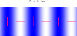
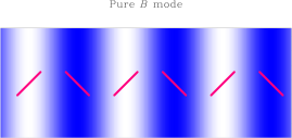
where angle brackets denote the symmetric, trace-free part, $\nabla_{a}$ is the covariant derivative on the sphere, and $\epsilon_{ab}$ is the alternating tensor. The divergence $\nabla^{a}\mathcal{P}_{ab}$ is a pure gradient if the magnetic part $P_{B}=0$, and a curl if the electric part $P_{E}=0$. The potential $P_{E}$ is a scalar under parity, but $P_{B}$ is a pseudo-scalar. For a given potential $P$, the electric and magnetic patterns it generates (i.e. with $P_{E}=P$ and $P_{B}=P$ respectively) are related by locally rotating the polarization directions by 45 degrees. The polarization orientations on a small patch of the sky for potentials that are locally Fourier modes are shown in Fig. 12. The potentials can be expanded in spherical harmonics (only the $l\geq 2$ multipoles contribute to $\mathcal{P}_{ab}$) as

$$P_{E}(\hat{\vec{n}})=\sum_{lm}\sqrt{\frac{(l-2)!}{(l+2)!}}E_{lm}Y_{lm}(\hat{\vec{n}})\;,\quad P_{B}(\hat{\vec{n}})=\sum_{lm}\sqrt{\frac{(l-2)!}{(l+2)!}}B_{lm}Y_{lm}(\hat{\vec{n}})\;.$$ (47)

(The normalisation is conventional.) Under parity $E_{lm}\rightarrow(-1)^{l}E_{lm}$ but $B_{lm}\rightarrow-(-1)^{l}B_{lm}$. Assuming rotational and parity invariance, $B$ is not correlated with $E$ or the temperature anisotropies $T$, leaving four non-vanishing power spectra: $C_{l}^{T}$, $C_{l}^{E}$, $C_{l}^{B}$ and the cross-correlation $C_{l}^{TE}$, where e.g. $\langle E_{lm}T_{lm}^{\ast}\rangle=C_{l}^{TE}$.

Figure 12: Polarization patterns for a pure-electric mode (left) and pure-magnetic mode (right) on a small patch of the sky for potentials that are locally Fourier modes. The shading denotes the amplitude of the potential. For the electric pattern the polarization is aligned with or perpendicular to the Fourier wavevector depending on the sign of the potential; for the magnetic pattern the polarization is at 45 degrees.

4.2 Physics of CMB Polarization

For scalar perturbations, the quadrupole of the temperature anisotropies at leading order in tight coupling is $\varTheta_{2}\sim k\dot{\tau}^{-1}v_{\gamma}$. Scattering of this quadrupole into the direction $-\hat{\vec{n}}$ generates linear polarization parallel or perpendicular to the projection of the wavevector $\vec{k}$ onto the sky, i.e. $\mathcal{P}_{ij}\sim\varTheta_{2}[\hat{k}_{\langle i}\hat{k}_{j\rangle}]^{\mathrm{TT}}$, where TT denotes the transverse (to $\hat{\vec{n}}$), trace-free part. In a flat universe the polarization tensor is conserved in the absence of scattering; for non-flat models this is still true if the components are defined on an appropriately-propagated basis (e.g. adc:challinor00 ). For a single plane wave perturbation, the polarization on the sky is thus purely electric (see Fig. 12). For tensor perturbations, the polarization $\mathcal{P}_{ij}\sim\dot{\tau}^{-1}[\dot{h}_{ij}]^{\mathrm{TT}}$ since the tightly-coupled quadrupole is proportional to the shear $\dot{h}_{ij}$. The gravitational wave defines additional directions on the sky when its shear is projected, and the polarization pattern is not purely electric. Thus density perturbations do not produce magnetic polarization in linear perturbation theory, while gravitational waves produce both electric and magnetic adc:seljak97 ; adc:kamionkowski97 .

Figure 13: Power spectra produced by adiabatic scalar perturbations (left) and tensor perturbations (right) for a tensor-to-scalar ratio $r=1$. On large scales the spectra from scalar perturbations are (from top to bottom) $C_{l}^{T}$, $C_{l}^{TE}$ and $C_{l}^{E}$. For tensor perturbations, they are $C_{l}^{T}$, $C_{l}^{TE}$, $C_{l}^{B}$ and $C_{l}^{E}$.

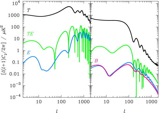
The polarization power spectra produced by scalar and tensor perturbations are compared in Fig. 13. The scalar $C_{l}^{E}$ spectrum peaks around $l\sim 1000$ since this corresponds to the projection of linear scales at last scattering for which diffusion generates a radiation quadrupole most efficiently. The polarization probes the photon bulk velocity at last scattering, and so $C_{l}^{E}$ peaks at the troughs of $C_{l}^{T}$, while $C_{l}^{TE}$ is zero at the peaks and troughs, and has its extrema in between. For adiabatic perturbations, the large-scale cross-correlation changes sign at $l\sim 50$, and, with the conventions adopted here is positive between $l=50$ and the first acoustic peak in $C_{l}^{T}$. Isocurvature modes produce a negative correlation from $l=2$ to the first acoustic trough.

Tensor modes produce similar power in electric and magnetic polarization. As gravitational waves damp inside the horizon, the polarization peaks just shortward of the horizon size at last scattering $l\sim 100$ despite these large scales being geometrically less efficient at transferring power to the quadrupole during a mean-free time than smaller scales.

For both scalar and tensor perturbations, the polarization would be small on large scales were it not for reionization, since a significant quadrupole is only generated at last scattering when the mean-free path approaches the wavelength of the fluctuations. However, reionization does produce significant large-angle polarization adc:zaldarriaga97 (see Fig. 13). The temperature quadrupole at last scattering peaks on linear scales with $k(\eta_{\mathrm{re}}-\eta_{*})\sim 2$, which then re-projects onto angular scales $l\sim 2(\eta_{0}-\eta_{\mathrm{re}})/(\eta_{\mathrm{re}}-\eta_{*})$. The position of the reionization feature is thus controlled by the epoch of reionization, and the height by the fraction of photons that scatter there i.e. $\tau_{\mathrm{re}}$. The measurement of $\tau_{\mathrm{re}}$ with large-angle polarization allows an accurate determination of the amplitude of scalar fluctuations from the temperature-anisotropy power spectrum. In addition, the fine details of the large-angle polarization power can in principle distinguish different ionization histories with the same optical depth, although this is hampered by the large cosmic variance at low $l$ adc:holder03 .

5 Highlights of Recent Results

In this section we briefly review some of the highlights from recent observations of the CMB temperature and polarization anisotropies. Analysis of the former have entered a new phase with the release of the first year data from the WMAP satellite adc:bennett03 ; a further three years worth of data are expected from this mission. Detections of CMB polarization are still in their infancy, but here too we can expect significant progress from a number of experiments in the short term.

5.1 Detection of CMB Polarization

Figure 14: Current measurements (as of February 2004) of $C_{l}^{TE}$ (top) and $C_{l}^{E}$ (bottom). The points with 1-$\sigma$ errors are from the first one-year data release from WMAP adc:hinshaw03 . The error boxes are the flat band-power results from DASI adc:kovac02 centred on the maximum-likelihood band power and spanning the 68-per cent interval. The solid lines are the predicted power from the best-fit model to all the WMAP data.

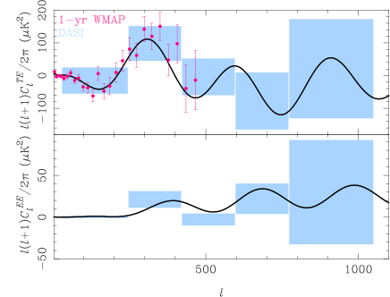
The first detection of polarization of the CMB was announced in September 2002 adc:kovac02 . The measurements were made with DASI, a compact interferometric array operating at 30 GHz, deployed at the South Pole. The DASI team constrained the amplitude of the $E$ and $B$-mode spectra with assumed spectral shapes derived from a concordant $\varLambda$CDM model. They obtained a $\sim 5$-$\sigma$ detection of a non-zero amplitude for $E$ with a central value perfectly consistent with that expected from the amplitude of the temperature anisotropies. DASI also detected the temperature–polarization cross-correlation at 95-per cent significance, but no evidence for $B$-mode polarization was found. The DASI results of a maximum-likelihood band-power estimation of the $E$ and $TE$ power spectra are given in Fig. 14.

Measurements of $C_{l}^{TE}$ were also provided in the first-year data release from WMAP, although polarization data itself was not released. These results are also shown in Fig. 14. The existence of a cross-correlation between temperature and polarization on degree angular scales provides evidence for the existence of super-horizon fluctuations on the last scattering surface at recombination. This is more direct evidence for such fluctuations than from the large-scale temperature anisotropies alone, since the latter could have been generated gravitationally all along the line of sight. The sign of the cross-correlation and the phase of its acoustic peaks relative to those in the temperature-anisotropy spectrum is further strong evidence for adiabatic fluctuations. The one surprise in the WMAP measurement of $C_{l}^{TE}$ is the behaviour on large scales. A significant excess correlation over that expected if polarization were only generated at recombination is present on large scales ($l<20$). The implication is that reionization occurred early, $11<z_{\mathrm{re}}<30$, giving a significant optical depth for re-scattering: $\tau_{\mathrm{re}}=0.17\pm 0.04$ at 68-per cent confidence. As mentioned in Sect. 2.5, reionization at this epoch is earlier than that expected from observations of quasar absorption spectra and suggests a complex ionization history.

5.2 Implications of Recent Results for Inflation

The generic predictions from simple inflation models are that: (i) the universe should be (very nearly) spatially flat; (ii) there should be a nearly scale-invariant spectrum of Gaussian, adiabatic density perturbations giving apparently-super-horizon fluctuations on the last scattering surface; and (iii) there should be a stochastic background of gravitational waves with a nearly scale-invariant (but necessarily not blue) spectrum. The amplitude of the latter is a direct measure of the Hubble rate during inflation, and hence, in slow-roll models, the energy scale of inflation.

As discussed in Sect. 3.2, the measured positions of the acoustic peaks constrains the universe to be close to flat. The constraint improves further with the inclusion of other cosmological data. There is no evidence for isocurvature modes in the CMB, although the current constraints are rather weak if general, correlated modes are allowed in the analysis adc:bucher04 . Several of the cosmological parameters for the isocurvature models most favoured by CMB data are violently at odds with other probes, most notably the baryon density which is pushed well above the value inferred from the abundances of the light-elements. There is also no evidence for primordial non-Gaussianity in the CMB (see e.g. adc:komatsu03 ).

Within flat $\varLambda$CDM models with a power-law spectrum of curvature fluctuations, the spectral index is constrained by the CMB to be close to scale invariant adc:spergel03 , although the inclusion of the latest data from small-scale experiments, such as CBI adc:readhead04 and VSA adc:rebolo04 , tends to pull the best fit from WMAP towards redder power-law spectra: e.g. $n_{\mathrm{s}}=0.97^{+0.06}_{-0.03}$ at 68-per cent confidence combining WMAP and VSA adc:rebolo04 . Slow-roll inflation predicts that the fluctuation spectrum should be close to a power law, with a run in the spectral index that is second order in slow roll: $\mathrm{d}n_{\mathrm{s}}/\mathrm{d}\ln k\sim(n_{\mathrm{s}}-1)^{2}$. The WMAP team reported weak evidence for a running spectral index by including small-scale data from galaxy redshift surveys and the Lyman-$\alpha$ forest, but modelling uncertainties in the latter have led many to question the reliability of this result (e.g. adc:seljak03 ). New data from CBI and VSA now provide independent evidence for running in flat $\varLambda$CDM models at the 2-$\sigma$ level from the CMB alone. This reflects the tension between the spectral index favoured by the low-$l$ CMB data (which is anomalously low for $l<10$, favouring bluer spectra) and the high-$l$ data from the interferometers. The evidence for running is weakened considerably with the inclusion of external priors from large-scale structure data. The best-fit values for the run in $n_{\mathrm{s}}$ obtained with the CMB alone are uncomfortably large for slow-roll inflation models, and give low power on small scales that is difficult to reconcile with the early reionization implied by the WMAP polarization data. However, a recent analysis adc:slosar04 argues that the evidence for running depends crucially on the techniques employed to estimate the low-$l$ power from WMAP data, and that the running is strongly suppressed if exact likelihood techniques are adopted. A definitive answer on whether departures from power-law spectra are significant must probably await further data on both large and small scales.

The final prediction of slow-roll inflation – the generation of nearly scale-invariant background of gravitational waves – is yet to be verified. The current limits on the tensor-to-scalar ratio are only weak: adc:rebolo04 report $r<0.68$ at 95-per cent confidence from all CMB data in general, non-flat, adiabatic $\varLambda$CDM models. Despite this, observations are beginning to place interesting constraints on specific models of inflation in the $r$–$n_{\mathrm{s}}$ plane adc:liddle03 ; adc:tegmark03 . Already, large-field models with power-law potentials steeper than $V\propto\phi^{6}$ are ruled out due to their red scalar spectra and comparatively large tensor-to-scalar ratio. Future programmes targeting $B$-mode polarization may ultimately be able to detect gravitational waves down to an inflationary energy scale of a $\mathrm{few}\times 10^{15}\,\mathrm{GeV}$. Such observations will sharpen constraints in the $r$–$n_{\mathrm{s}}$ plane considerably, and should allow fine selection amongst the many proposed models of inflation.

5.3 Detection of Late-Time Integrated Sachs-Wolfe Effect

The late-time ISW effect arises from the decay of the gravitational potentials once the universe becomes dark-energy dominated, and so should produce large-angle (positive) correlations between the CMB temperature anisotropies and other tracers of the potential in the local universe. With the advent of the WMAP data, a number of groups have reported the detection of such a correlation. In adc:boughn04 , WMAP data was cross-correlated with data on the hard X-ray background (which is dominated by emission from active galaxies) from the HEAO-1 satellite, and the number density of radio sources from the NVSS catalogue. In each case a positive correlation was detected at significance $3\sigma$ and $2.5\sigma$ respectively. The correlation with NVSS has also been carried out independently by the WMAP team adc:nolta03 , who also note that the observed positive correlation can be used to rule out the closed, $\varLambda=0$ model model that is a good fit to the CMB data in isolation (see Fig. 11). Several groups have now also detected the cross-correlation on large scales between the CMB and optical galaxy surveys, e.g. adc:fosalba03 .

6 Conclusion

The linear anisotropies of the cosmic microwave background have been studied theoretically for over three decades. The physics, which is now well understood, employs linearised radiative transfer, general relativity, and hydrodynamics to describe the propagation of CMB photons and the evolution of the fluid constituents in a perturbed Friedmann-Robertson-Walker universe. A number of bold predictions have emerged from this theoretical activity, most notably the existence of acoustic peaks in the anisotropy power spectrum due to oscillations in the photon–baryon plasma prior to recombination. Observers have risen to the challenge of verifying these predictions, and their detection is proceeding at a staggering rate. The large-scale Sachs–Wolfe effect, acoustic peak structure, damping tail, late-time integrated Sachs–Wolfe effect, polarization and reionization signature have all been detected, and the first three have been measured in considerable detail. Already, the size and scale of these effects is allowing cosmological models to be constrained with unprecedented precision. The results are beautifully consistent with almost-scale-invariant adiabatic initial conditions evolving passively in a spatially flat, $\varLambda$CDM universe.

Much work still remains to be done to exploit fully the information contained in the CMB anisotropies. The Planck satellite, due for launch in 2007, should provide definitive mapping of the linear CMB anisotropies, and a cosmic-variance limited measurement of the power spectrum up to multipoles $l\sim 2000$. This dataset will be invaluable in assessing many of the issues hinted at in the first-year release of WMAP data, such as the apparent lack of power on large scales and possible violations of rotational (statistical) invariance. Prior to Planck, a number of ground-based programmes should shed further light on the issue of whether departures from a power-law primordial spectrum are required on cosmological scales, and the implications of this for slow-roll inflation. In addition, these small-scale observations will start to explore the rich science of secondary anisotropies, due to e.g. scattering in hot clusters adc:sz72 or bulk flows modulated by variations in the electron density in the reionized universe adc:sz80 ; adc:ostriker86 , and the weak lensing effect of large-scale structure adc:blanchard87 .

Detections of CMB polarization are in their infancy, but we can expect rapid progress on this front too. Accurate measurements of the power spectra of $E$-mode polarization, and its correlation with the temperature anisotropies, can be expected from a number of ground and balloon-borne experiments, as well as from Planck. The ultimate goal for CMB polarimetry is to detect the $B$-mode signal predicted from gravitational waves. This would give a direct measure of the energy scale of inflation, and, when combined with measurements of the spectrum density perturbations, place tight constraints on the dynamics of inflation. Plans are already being made for a new generation of polarimeters with the large numbers of detectors and exquisite control of instrument systematics needed to detect the gravity-wave signal if the energy scale of inflation is around $10^{16}\,\mathrm{GeV}$. Ultimately, confusion due to imperfect subtraction of astrophysical foregrounds and the effects of weak lensing on the polarization limit will limit the energy scales that we can probe with CMB polarization; see adc:hirata03 and references therein.

References

- (1) A.A. Penzias, R.W. Wilson: Astrophys. J. 142, 419 (1965)
- (2) R.H. Dicke et al: Astrophys. J. 142, 414 (1965)
- (3) R.K. Sachs, A.M. Wolfe: Astrophys. J. 147, 73 (1967)
- (4) G.F. Smoot et al: Astrophys. J. Lett. 396, 1 (1992)
- (5) P.J.E. Peebles: Astrophys. J. Lett. 263, 1 (1982)
- (6) J.R. Bond, G. Efstathiou: Astrophys. J. Lett. 285, 45 (1984)
- (7) P.J.E. Peebles J.T. Yu: Astrophys. J. 162, 815 (1970)
- (8) J.C. Mather et al: Astrophys. J. 420, 439 (1994)
- (9) J.C. Mather et al: Astrophys. J. 512, 511 (1999)
- (10) J.R. Bond, C.R. Contaldi, D. Pogosyan: Phil. Trans. Roy. Soc. Lond. A 361, 2435 (2003)
- (11) C.L. Bennett et al: Astrophys. J. Suppl. 148, 1 (2003)
- (12) D.N. Spergel et al: Astrophys. J. Suppl. 148, 175 (2003)
- (13) J.M. Kovac et al: Nature 420, 772 (2002)
- (14) W. Hu, S. Dodelson: Ann. Rev. Astron. Astrophys. 40, 171 (2002)
- (15) W. Hu: Ann. Phys. 303, 203 (2003)
- (16) P.J.E. Peebles: Astrophys. J. 153, 1 (1968)
- (17) Y.B. Zeldovich, V.G. Kurt, R.A. Syunyaev: Journal of Experimental and Theoretical Physics 28, 146 (1969)
- (18) S. Seager, D.D. Sasselov, D. Scott: Astrophys. J. Suppl. 128, 407 (2000)
- (19) A. Kogut et al: Astrophys. J. Suppl. 148, 161 (2003)
- (20) C. Dickinson et al: preprint astro-ph/0402498, (2004).
- (21) B.S. Mason et al: Astrophys. J. 591, 540 (2003)
- (22) T.J. Pearson et al: Astrophys. J. 591, 556 (2003)
- (23) C.L. Kuo et al: Astrophys. J. 600, 32 (2004)
- (24) C.W. Misner, K.S. Thorne, J.A. Wheeler: Gravitation, (W. H. Freeman and Company, San Francisco 1973) pp 583–590
- (25) W. Hu et al: Phys. Rev. D 57, 3290 (1998)
- (26) A. Challinor: Phys. Rev. D 62, 043004 (2000)
- (27) G.F.R. Ellis, J. Hwang, M. Bruni: Phys. Rev. D 40, 1819 (1989)
- (28) A. Challinor, A. Lasenby: Astrophys. J. 513, 1 (1999)
- (29) A. Challinor: Class. Quantum Grav. 17, 871 (2000)
- (30) R. Maartens, T. Gebbie, G.F.R. Ellis: Phys. Rev. D 59, 083506 (1999)
- (31) T. Gebbie, G.F.R. Ellis: Ann. Phys. 282, 285 (2000)
- (32) T. Gebbie, P.K.S. Dunsby, G.F.R. Ellis: Ann. Phys. 282, 321 (2000)
- (33) C. Ma, E. Bertschinger: Astrophys. J. 455, 7 (1995)
- (34) M. Bartelmann, P. Schneider: Phys. Rep. 340, 291 (2001)
- (35) M.L. Wilson: Astrophys. J. 273, 2 (1983)
- (36) U. Seljak, M. Zaldarriaga: Astrophys. J. 469, 437 (1996)
- (37) A. Lewis, A. Challinor, A. Lasenby: Astrophys. J. 538, 473 (2000)
- (38) N. Kaiser: Mon. Not. R. Astron. Soc. 202, 1169 (1983)
- (39) W. Hu, N. Sugiyama: Astrophys. J. 444, 489 (1995)
- (40) W. Hu, N. Sugiyama: Phys. Rev. D 51, 2599 (1995)
- (41) M. Bucher, K. Moodley, N. Turok: Phys. Rev. D 62, 083508 (2000)
- (42) L. Page et al: Astrophys. J. Suppl. 148, 233 (2003)
- (43) C. Gordon, A. Lewis: Phys. Rev. D 67, 123513 (2003)
- (44) M. Bucher et al: preprint astro-ph/0401417, (2004)
- (45) J. Silk: Astrophys. J. 151, 459 (1968)
- (46) J.M. Stewart: Class. Quantum Grav. 7, 1169 (1990)
- (47) S. Boughn, R. Crittenden: Nature 427, 45 (2004)
- (48) M.R. Nolta et al: preprint astro-ph/0305097, (2003)
- (49) P. Fosalba, E. Gaztañaga and F.J. Castander: Astrophys. J. Lett. 597, 89 (2003)
- (50) R.H. Becker et al: Astron. J. 122, 2850 (2001)
- (51) S.G. Djorgovski et al: Astrophys. J. Lett. 560, 5 (2001)
- (52) U. Seljak, M. Zaldarriaga: Phys. Rev. Lett. 78, 2054 (1997)
- (53) M. Kamionkowski, A. Kosowsky, A. Stebbins: Phys. Rev. Lett. 78, 2058 (1997)
- (54) J.R. Bond et al: Phys. Rev. Lett. 72, 13 (1994)
- (55) L.F. Abbott, R.K. Schaefer: Astrophys. J. 308, 546 (1986)
- (56) G. Efstathiou, J.R. Bond: Mon. Not. R. Astron. Soc. 304, 75 (1999)
- (57) A.G. Riess et al: Astron. J. 116, 1009 (1998)
- (58) S. Perlmutter et al: Astrophys. J. 517, 565 (1999)
- (59) W.L. Freedman et al: Astrophys. J. 553, 47 (2001)
- (60) A. Lewis, A. Challinor, N. Turok: Phys. Rev. D 65, 023505 (2002)
- (61) M. Zaldarriaga: Phys. Rev. D 55, 1822 (1997)
- (62) G. Holder et al: Astrophys. J. 595, 13 (2003)
- (63) G. Hinshaw et al: Astrophys. J. Suppl. 148, 135 (2003)
- (64) E. Komatsu et al: Astrophys. J. Suppl. 148, 119 (2003)
- (65) A. de Oliveria-Costa et al: preprint astro-ph/0307282, (2003)
- (66) P. Vielva et al: preprint astro-ph/0310273, (2003)
- (67) C.J. Copi, D. Huterer, G.D. Starkman: preprint astro-ph/0310511, (2003)
- (68) H.K. Eriksen et al: preprint astro-ph/0401276, (2004)
- (69) F.K. Hansen et al: preprint astro-ph/0402396, 2004.
- (70) A.C.S. Readhead et al: preprint astro-ph/0402359, (2004)
- (71) R. Rebolo et al: preprint astro-ph/0402466, (2004)
- (72) U. Seljak, P. McDonald, A. Makarov: Mon. Not. R. Astron. Soc. 342, L79 (2003)
- (73) A. Slosar, U. Seljak, A. Makarov: preprint astro-ph/0403073, (2004)
- (74) S.M. Leach, A.R. Liddle: Mon. Not. R. Astron. Soc. 341, 1151 (2003)
- (75) M. Tegmark et al: preprint astro-ph/0310723, (2003)
- (76) R.A. Sunyaev, Y.B. Zeldovich: Comm. Astrophys. Space Phys. 4, 173 (1972)
- (77) R.A. Sunyaev, Y.B. Zeldovich: Mon. Not. R. Astron. Soc. 190, 413 (1980)
- (78) J.P. Ostriker, E.T. Vishniac: Astrophys. J. Lett. 306, 51 (1986)
- (79) A. Blanchard, J. Schneider: Astron. Astrophys. 184, 1 (1987)
- (80) C.M. Hirata, U. Seljak: Phys. Rev. D 68, 083002 (2003)