Raising the Dead: Clues to Type Ia Supernova Physics from the Remnant 0509$-$67.5

Abstract

We present Chandra X-ray observations of the young supernova remnant (SNR) 0509$-$67.5 in the Large Magellanic Cloud (LMC), believed to be the product of a Type Ia supernova (SN Ia). The remnant is very round in shape, with a distinct clumpy shell-like structure that extends to an average radius of $14.8\arcsec$ (3.6 pc) in the X-ray band. Our Chandra data reveal the remnant to be rich in silicon, sulfur, and iron. The yields of our fits to the global spectrum confirm that 0509$-$67.5 is the remnant of an SN Ia and show a clear preference for delayed detonation explosion models for SNe Ia. The Chandra spectra extracted from radial rings are in general quite similar; the most significant variation with radius is a drop in the equivalent widths of the strong emission lines right at the edge of the remnant. We study the spectrum of the single brightest isolated knot in the remnant and find that it is enhanced in iron by a factor of roughly two relative to the global remnant abundances. This feature, along with similar knots seen in Tycho’s SNR, argues for the presence of modest small-scale composition inhomogeneities in SNe Ia. The presence of both Si and Fe, with abundance ratios that vary from knot to knot, indicates that these came from the transition region between the Si- and Fe-rich zones in the exploded star, possibly as a result of energy input to the ejecta at late times due to the radioactive decay of ⁵⁶Ni and ⁵⁶Co. Two cases for the continuum emission from the global spectrum were modeled: one where the continuum is dominated by hydrogen thermal bremsstrahlung radiation; another where the continuum arises from non-thermal synchrotron radiation. The former case requires a relatively large value for the ambient density ($\sim$1 cm^-3). Another estimate of the ambient density comes from using the shell structure of the remnant in the context of dynamical models. This requires a much lower value for the density ($<$0.05 cm^-3) which is more consistent with other evidence known about 0509$-$67.5. We therefore conclude that the bulk of the continuum emission from 0509$-$67.5 has a non-thermal origin.

1 INTRODUCTION

Type Ia supernovae (SN Ia) are characterized by the absence of Balmer lines and the presence of strong silicon lines in their optical spectra (Hillebrandt & Niemeyer, 2000). They yield mostly intermediate mass elements from Si to Ca and are the main sources of iron production in galaxies. Each SN Ia produces $\sim$0.8 ${\rm M{{}_{\sun}}}$ of Fe (Iwamoto et al., 1999), making them important for understanding the chemical evolution of galaxies. The peak magnitude and shape of their light curves are fairly homogeneous, which makes them useful as distance indicators and tools for cosmology (Riess, Press, & Kirshner, 1996; Riess et al., 1998; Perlmutter et al., 1999). For these reasons, SN Ia’s are the objects of much study.

Still, there is much that remains uncertain about them. The progenitors of SN Ia’s are believed to be degenerate C+O white dwarfs. Although models for sub-Chandrasekhar mass explosions exist, the favored explanation is that the degenerate object somehow exceeds the Chandrasekhar limit before exploding. Two possibilities include a single degenerate scenario, in which the white dwarf accretes mass from a companion star, and a double degenerate scenario, in which a pair of white dwarfs coalesce (Branch et al., 1995). It is still unclear whether one, both, or none of these offers the correct explanation. In addition, the mechanism of the explosion, i.e., where the ignition begins and how it propagates outward, continues to elude us (Iwamoto et al., 1999). Two cases studied in detail include a fast deflagration and a delayed detonation. In the former, a deflagration begins close to the center of the progenitor star and propagates subsonically. The delayed detonation case involves a deflagration initially, which is transformed at some density to a detonation as the star expands. Models for these two cases are parameterized by the speed of the burning front and the location of the ignition in density space; we compare our results with those of Iwamoto et al. (1999).

By studying the remnants of SN Ia explosions, we can hope to gather clues to some of these puzzles. The supernova remnant (SNR) 0509$-$67.5 in the Large Magellanic Cloud (LMC) is believed to be the remnant of an SN Ia (Tuohy et al., 1982; Hughes et al., 1995). It was discovered in an X-ray survey of the LMC with the Einstein X-ray Observatory (Long, Helfand, & Grabelsky, 1981). However, much of the previous study on this remnant was done via optical spectroscopy. In H$\alpha$, the remnant appears as a very circular shell (Tuohy et al., 1982). 0509$-$67.5 shows no detectable emission in [O III] and [S II], indicating it is a Balmer-dominated remnant (Tuohy et al., 1982; Smith et al., 1991; Smith, Raymond, & Laming, 1994). Remnants such as this generally have two components to the H$\alpha$ emission line: a narrow component produced by neutral hydrogen being excited by the shock, and a broad component produced by charge exchange with fast protons post-shock. In 0509$-$67.5, Smith et al. (1994) found the narrow components to be $\sim$25–31 km/s, higher than expected for neutral hydrogen and a possible indication of the presence of a cosmic ray precursor. This SNR is also intriguing in that its broad component is believed to be so broad that it has escaped detection, pointing to very fast shocks ($\geq$2000 km/s) and a young age ($\leq$1000 yr) (Smith et al. 1991; Smith et al. 1994). Tuohy et al. (1982) found that 0509$-$67.5 is expanding into a low density medium, with $n_{\rm H}\lesssim 0.02$ cm^-3. A previous X-ray study of this SNR with ASCA revealed it to be strong in Si and Fe L emission, with little O, Ne, and Mg emission (Hughes et al., 1995). This remnant has also been observed in the radio, showing a spectral index of $\alpha=0.46$ (Mathewson et al., 1983) and a flux density of 0.066 Jy at 1 GHz (Hendrick & Reynolds, 2001).

2 OBSERVATIONS

0509$-$67.5 was observed with the Chandra X-ray Observatory for 51.4 ks on 2000 May 12-13 on the back-side–illuminated chip (S3) of the Advanced CCD Imaging Spectrometer (ACIS-S) (Obs ID 776). We made use of the charge transfer inefficiency (CTI) corrector code (Townsley et al., 2000) to correct for spatial gain variations. Standard software tools were used to filter for grade (retaining the usual grades 02346 only), bad pixels, and times of high or flaring background. After all filtering, the net exposure time was 47.9 ks. All spectral analyses utilized the pulse-invariant (PI) column of the final Chandra events file.

As described in §4.1.1 as well as in Hughes et al. (1995), the spectrum of 0509$-$67.5 includes a strong Si line. We measured the centroid of this Si K$\alpha$ line to be low, $1.835\pm 0.002$ keV, which is indicative of a very low ionization state for Si, i.e., Li- or Be-like. Most SNRs generally show either the H-like Si K$\alpha$ transition at 2 keV or the He-like Si K$\alpha$ complex at $\sim$1.86 keV.

Chandra has onboard radioactive sources for calibration, which we used to independently verify the energy scale of the detector at the time of the 0509$-$67.5 observation. Two calibration observations (Obs IDs 62057 and 62058) were taken just prior to ours, and two more (62055 and 62056) were taken beginning the day after. After running the CTI corrector code on these data, we fit gaussian lines to the spectra of the sources. The most prominent lines were Al K$\alpha$, Ti K$\alpha$, Mn K$\alpha$, and Mn K$\beta$. The centroids of these lines were compared with the accepted values (Lide, 1995) and found to have less than 0.2% difference. Most of the centroid values agree with the accepted values within the errors (see Table 1). The residual uncertainty in the energy scale is of order a few eV at both $\sim$1.5 keV and $\sim$6.5 keV, which is the order of the uncertainty in our Si line centroid. Therefore, we can be confident that we do indeed have a low ionization state for Si.

3 IMAGING

3.1 Chandra Image

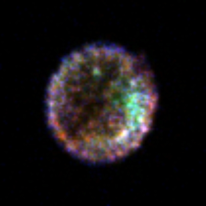
Figure 1: The 3-color Chandra broadband (0.2–7 keV) X-ray image of 0509$-$67.5. The image has been smoothed with a gaussian with a sigma of $\sim 0.25\arcsec$. Red contains emission from 0.2–0.69 keV, green 0.69–1.5 keV, and blue 1.5–7 keV. North is up and east is to the left.

In Figure 1 we present the 3-color Chandra broadband (0.2–7 keV) X-ray image of 0509$-$67.5. Red contains emission from 0.2–0.69 keV, green 0.69–1.5 keV, and blue 1.5–7 keV. The image reveals a clear shell of emission which is very circular, with a slight break in the northwest. The shell itself appears clumpy, with small knots of emission spaced seemingly periodically around the bright rim. In fact, most of the structure in this remnant can be characterized as clumpy, as there are no filaments or elongated features visible. On the northern portion of the rim and more faintly on the southern portion, the higher energy band emission is slightly enhanced. In the southeast, we see some enhancement in the lower energy band. The rest of the rim shows less spectral variation. Most of the interior shows only faint emission, except for an enhanced clumpy region in the southwest and a lone knot in the north, both clearly dominated by the middle energy range, where Fe L emission is strong. There seem to be two distinct halves to the SNR, the dividing line running at an angle of $\sim$30$\arcdeg$ west of north.

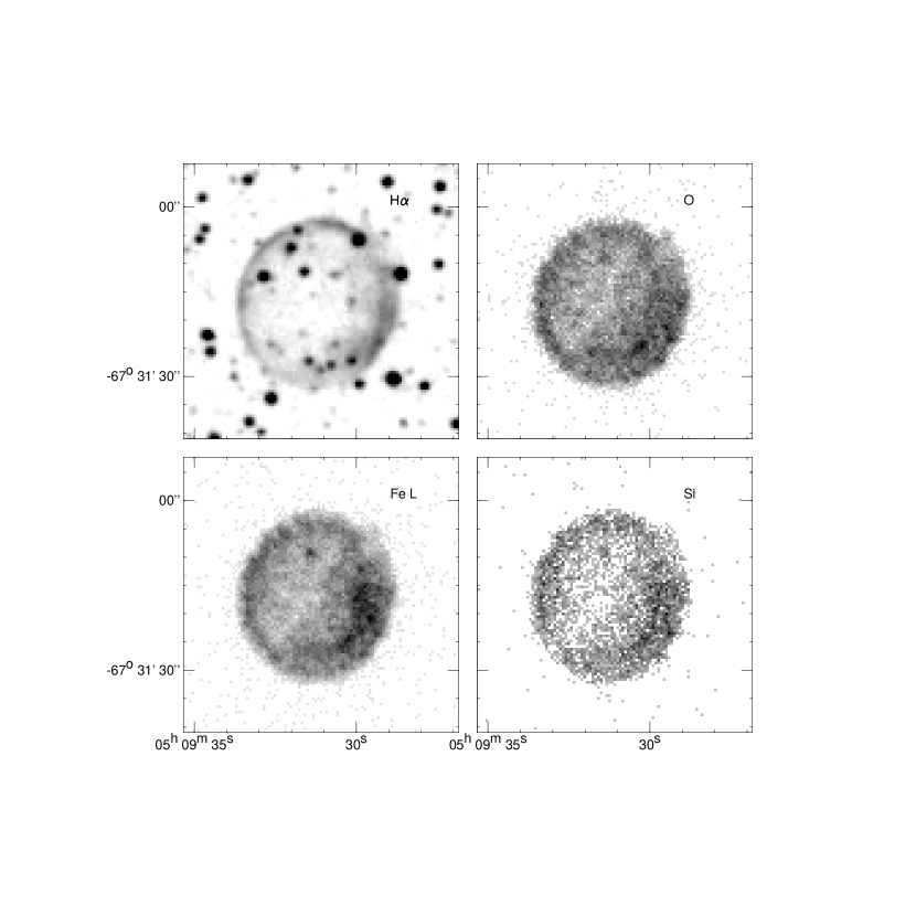
Figure 2: CTIO 4-m H$\alpha$ image of 0509$-$67.5 (upper left), Chandra Oxygen 0.45–0.7 keV image (upper right), Iron L 0.7–1.4 keV image (lower left), and Silicon 1.5–2 keV image (lower right). The intensity to grayscale mapping is square root. North is up and east is to the left.

Separating the different energy bands, as presented in Figure 2, reveals essentially the same subtle variations as noted in the color image. Here we chose narrower spectral bands that contain emission mostly from O (0.45–0.7 keV), Fe L (0.7–1.4 keV), and Si (1.5–2 keV). In the O band, the knot in the north and the clumpy region in the southwest are much fainter. The rim here is less apparent than in the other bands, although there does seem to be a slight enhancement in the southeast, present in the color image as well. The brightness of the interior emission is also more uniform here. As before, the Fe L band reveals the clumpy region and knot to be quite prominent, and it is in this energy band that these spatial features are most obvious. The Si band shows fainter emission in the interior. The knot and clumpy region are apparent here, and the northeastern rim appears slightly brighter at these energies. Spectral differences within the remnant are small and are mostly associated with the knot, clumpy region, and outermost edge (see §4.2). The CTIO 4-m H$\alpha$ image (Smith et al., 1991) also reveals a shell of emission, with slight enhancements in the north and southwest, and a fainter area in the southeast. There is virtually no H$\alpha$ in the interior.

3.2 Image Fits

The distinct shell-like nature of the remnant prompted us to investigate this structure further. We did this in two ways: fitting a simple geometric model to the image, and performing a deprojection of the normalizations derived from spatially-resolved spectra, which is described in §5. Our specific goals for the simple image fits were modest: (1) to determine the inner and outer radii of the shell of X-ray emitting material, and (2) to estimate the total SNR X-ray flux that comes from clearly resolved bright knots. We used a model consisting of two nested elliptical shells and a number of spherical knots that describe the observed X-ray surface brightness of the SNR. Each individual component was assumed to be optically thin and have uniform emissivity, so that the projected surface brightness distribution was uniquely determined by the geometry of the model. The shell models shared the same center, axial ratio, and position angle for the major axis, assumed to lie in the plane of the sky. The inner edge of the outer shell and the outer edge of the inner shell were set equal (i.e., the shells were adjoining). Thus, in total there were nine parameters for the shell models: the center position in R.A. and declination, axial ratio, position angle, outer radius of the outer shell, common radius, inner radius of the inner shell, and the intrinsic emissivities of the outer and inner shells. Each spherical knot required four parameters: center position in R.A. and declination, radius, and intrinsic emissivity. The model surface brightness was convolved with the Chandra point spread function (PSF) appropriate to the center of the SNR at a monochromatic energy of 0.75 keV (where the observed spectrum peaks). The PSF was determined using the Chandra Ray Tracing (ChaRT) program (described in §5). Only the symmetric northeastern portion of the SNR was fit to avoid complications with the clumpy region just inside the main shell visible on the southwestern side.

The software we used is described in Hughes & Birkinshaw (1998). It is based on a maximum likelihood figure of merit function derived for Poisson-distributed data and allows for the determination of both best-fit parameter values as well as confidence intervals. We employ the robust downhill simplex method (Press et al., 1985) for function minimization.

Fits were done in an iterative fashion, starting with the shell models alone and then adding successively more and more spherical knots, as needed. Knot models were introduced at the locations of the most significant residuals between the data and the model from the previous iteration. Iterations were continued until the absolute value of the residuals fell below $\sim$10 X-ray events/pixel. Knots representing regions of excess emission (positive residuals) were modeled with positive intrinsic emissivity values. We also allowed for negative emissivity knots to account for negative residuals, i.e., regions of lower overall emission. The physical interpretation is that these knots represent places in the shell with lower than average density or thickness that appear faint relative to their surroundings. In models with such negative knots, the overall modeled surface brightness was required to be non-negative everywhere before PSF convolution in order to ensure a physically realistic model.

The shell model is intended to describe the overall limb-brightened, global structure of the remnant, and the knots represent additional intensity fluctuations on spatial scales of an arcsecond or so. Due to the simplicity of the geometric structure models and the large number of arbitrary free parameters (e.g., four for each knot model), our image fitting procedure does not lead to a unique solution for the structure of the remnant. In addition we found that the precise manner in which knot models were introduced resulted in noticeable differences in the derived remnant structure. However, our intent here is not to derive a unique spatial model, but rather one that is broadly representative of the spatial distribution of X-ray flux from 0509$-$67.5. The shell and spherical knot models provide a convenient way to parameterize this. We experimented with different methods for introducing models during the iterative fitting process and found that our quantities of interest (the inner and outer radii of the shell model and the average ratio of number of X-ray events to volume for the knots) were fairly robust against variations in the fitting procedure.

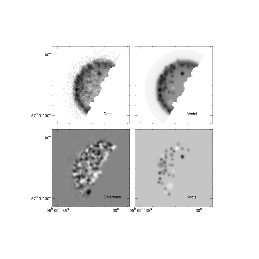
Figure 3: Image fits to the northeast half of the remnant. The upper left panel shows the broadband Chandra image. The model, including knots, is shown in the upper right, and the difference between the model and the data is in the lower left. The lower right panel displays the knot model alone. The intensity range of the grayscale in the data and model panels is 0 to 100 X-ray events per pixel, the difference panel is $-$10 to 10 events per pixel, while the knots panel ranges over values of $-$10 to 90 events per pixel. North is up and east is to the left.

Figure 3 shows the results of the image fits. One measure of the success of our image fitting procedure is the good agreement between the “Data” and “Model” panels in the figure. In this best-fit model there are 28 knots of positive emission and 5 knots of negative emission. Most of the knots are effectively unresolved (i.e., fitted sizes less than or comparable to the Chandra PSF) and appear to be distributed non-uniformly over the portion of the image fitted. However, the radial distribution of knots is consistent with that expected for a uniform distribution within the volume of a thin spherical shell. Comparison of the FFT power spectra of the raw data image and best-fit model reveal the presence of additional significant power in the data, above Poisson noise, on the smallest spatial scales. Further support for this is evident in the “Difference” panel of Figure 3, which we interpret as showing intensity fluctuations on smaller spatial scales. Thus our image fits have only captured the brightest and most obvious small-scale structure in the image and what we have modeled as diffuse shell-like emission actually consists of knots extending to scales below our image resolution. This is most likely similar to the “fleecey” structure evident in Chandra images of Tycho’s SNR, which may be a typical feature of SN Ia remnants.

There were 38,900 X-ray events in the fitted portion of the image. The fit yielded 11,100 (21,600) in the outer (inner) shell, 6800 in positive knots, $-$900 in negative knots and roughly 100 in background. (The values do not sum due to rounding.) Of most interest is the relationship between the number of detected X-ray events and the geometric volume of the component. In particular we want to compare the number of events and the volume from the knot component to that of the shell component. Using the above values, the ratio of X-ray events in the positive knots to the shells is $\sim$20%. The volume corresponding to the sum of all the fitted knots is only 2% of the total volume of the shell component. We use these values in §6.4 below.

The inner and outer radii (more precisely the semi-major axis lengths) of the shells determined from our fits are 15.2$\arcsec$ and 12.8$\arcsec$, which correspond to physical radii of 3.69 pc and 3.10 pc for an LMC distance of 50 kpc (assumed throughout). The axial ratio for the elliptical shells is 0.945 and the major axis lies at a position angle of 7.6$\arcdeg$ west of north. The outer edge of the X-ray emitting shell corresponds nearly perfectly with the outer edge of the H$\alpha$ image of 0509$-$67.5 from Smith et al. (1991). This indicates that the outer edge of the X-ray emission corresponds to the location of the blast wave propagating into the interstellar medium. We suggest that the inner edge of the X-ray emitting shell corresponds to the location of the reverse shock propagating backward into the ejecta.

4 SPECTRA

4.1 Global Spectrum

We describe the model fits to the global, or integrated, spectrum of 0509$-$67.5 (see Figure 4) in some detail. The global spectrum provides us with the elemental yields for this remnant, which we will use to argue for a Type Ia origin (see §6.1). In addition, the best-fit models for this spectrum are used as templates for the spectra of half-ring regions used to determine the shell structure of 0509$-$67.5 (see §4.2).

4.1.1 Basic Model Fits

It was immediately apparent that 0509$-$67.5 was rich in Si, as evidenced by a strong Si K$\alpha$ emission line in the global spectrum (see Figure 4). Because of this, we attempted to fit the high end ($>$1.6 keV) portion of the spectrum and then extrapolate back for the lower energies utilizing the minimum number of free parameters necessary to obtain a good fit. This regime includes K-shell lines of Si, S, Ar, Ca, and Fe, while excluding the strong Fe L-shell emission, for which the atomic physics is not as well understood. We used a non-equilibrium ionization (NEI) plane-parallel shock model (Hughes, Rakowski, & Decourchelle, 2000) to do the fitting, allowing column density, temperature, terminal value of the ionization timescale, and the elemental abundances of Si, S, Ar, Ca and Fe to vary freely. Abundances are relative to the solar values of Anders & Grevesse (1989). Hydrogen was used to model the continuum, and no other species were included. LMC abundances of 0.3 times solar were used to determine the column density, and an additional Galactic column density of $5.5\times 10^{20}$ cm^-2 (Dickey & Lockman, 1990) was incorporated at solar abundances. The spectrum was background subtracted using an annular region surrounding the SNR.

We obtained good fits to the high energy portion of the spectrum with abundances given in Table 2, as long as Si was allowed a slightly lower ionization timescale than the other elements, and Fe was allowed both a higher temperature and higher ionization timescale. However, this particular fit overpredicted the emission below $\sim$ 1 keV. In order to fit the lower energies, we added in O, Ne, and Mg. We then stepped through the temperature until we found a good fit. The temperature increased from the best value of the high energy fit, while the ionization timescales decreased (this significantly improved the fit below 1 keV). The abundances of Si, S, and Ar decreased only slightly; Ca showed a more pronounced decrease, and Fe went up (see Table 2). While the fits definitely required O and Mg emission, adding Ne resulted in no improvement. There was a need for a line at 2.11 keV that was not included in the NEI model. We believe this to be a K$\beta$ line of Si, which we fit with a gaussian line.

There was also a portion of the spectrum around 0.73 keV, presumably Fe L-shell emission, which the model could not fit. It was possible to compensate for this deficiency by including a single narrow gaussian line with freely varying energy centroid and intensity. Because this is the brightest part of the spectrum, the $\chi^{2}$ statistic weights data points in this vicinity more than those at lower or higher energies, even though our understanding of the atomic physics here is poorest. We therefore introduced a systematic error of 5% to the data so that our reduced-$\chi^{2}$ value was 1, and the statistical weight of points near the Fe L-shell emission was reduced. An advantage of having a reduced-$\chi^{2}$ = 1 is that we can derive errors on fitted quantities in the usual manner. We should stress that while there are inadequacies in the model, it still does a good job of fitting the rest of the Fe L emission which extends from $\sim$0.8–1.3 keV, as well as the K-shell emission lines. So, while the model could be more accurate in some regions, we are confident that it is good overall.

4.1.2 Two Models of Continuum

Continuum emission in SNRs can come about in various ways. It could arise from the metals in the ejecta alone. However, the equivalent widths of the line emission we see in 0509$-$67.5 are not as high as we would expect to see in this case, so another source of continuum emission is required. The thermal bremsstrahlung radiation of electrons on ionized hydrogen, from either the interstellar medium (ISM) or the ejecta itself, can produce sufficient continuum emission. We modeled this case with hydrogen as the continuum component (hereafter, Case H). We assumed the continuum temperature and the temperatures of the metals, excepting Fe, were the same. No He or other species were added to the continuum model as we were attempting to fit our spectrum with the least number of physically plausible parameters.

A second case we modeled was for non-thermal X-ray synchrotron radiation. SN1006 and other SNRs show approximately power-law spectra in the X-ray band which is now believed to be the signature of a population of relativistic particles accelerated by the SN shocks (Koyama et al., 1995; Allen et al., 1997). It has been observed that this X-ray power-law spectrum steepens from the power-law at radio frequencies. Simple parameterized models have been developed to account for this. One such is the synchrotron cut-off (SRCUT) model, that takes as input the radio flux at 1 GHz and the radio spectral energy index, and fits for the so-called “roll-off” (or “cut-off”) frequency. This is the frequency at which the X-ray flux has fallen to about a factor of 10 below the extrapolated radio spectrum (Reynolds & Keohane, 1999). The SRCUT model was applied to 0509$-$67.5 by Hendrick & Reynolds (2001) using archival ASCA and radio data, and they obtained an upper limit to the roll-off frequency of 2.9$\times 10^{16}$ Hz. Using our Chandra data, we applied the SRCUT model in the context of our global fit (hereafter, Case S) and were able to get good fits to our spectrum. In addition, our result for $\nu_{roll-off}=1.6\times 10^{16}$ Hz falls well below their limit. We also fit a power-law model to the spectrum in place of the SRCUT model to obtain the photon index. A value of $3.25\pm 0.18$ and a normalization at 1 keV of $2.2\times 10^{-7}$ Jy fit the data well.

In Figure 4, we plot the global spectrum of 0509$-$67.5 overlaid with the best-fit Case H (solid line) and Case S (dotted line) models. Up to about 3 keV the two models are virtually indistinguishable. Above 3 keV, Case H overpredicts the continuum level and Case S fits the data better. In Table 3 we present the best-fit parameters for Cases H and S for the global spectrum. Here, $n_{e}n_{i}V/$[i/H]_☉ is the emission measure (EM) of each species, $i$, relative to the solar abundance for that species. This was done so that if we were looking at a solar plasma, the quantities listed would all have the same value. For Case H we can also determine absolute abundances relative to solar; those values are given in the last column of Table 2. For Case S this is not possible since we have set the EM of hydrogen to zero. Other than that, there are no glaring differences in EMs between the two cases. In general, Case S shows slightly lower EMs than Case H. The temperature for Case S is a bit higher, as well. As mentioned in §4.1.1, we included a systematic error in our data when fitting for Case H. This was carried over into our fits for Case S, but in fact may be a slight overestimate for this case (since the overall fit is somewhat better for Case S).

4.2 Ring Spectra

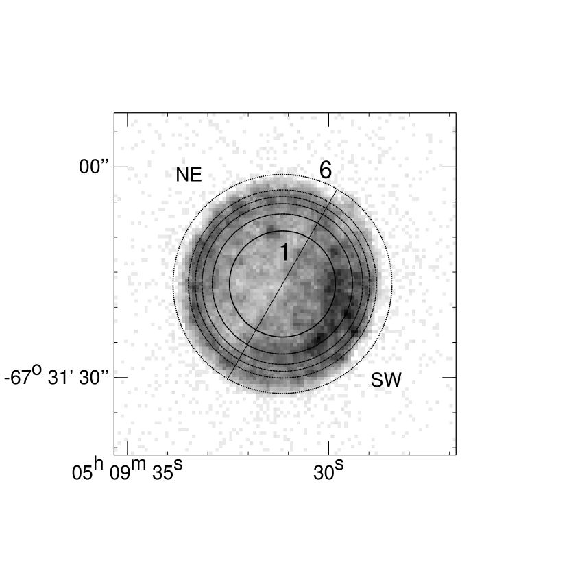
Figure 5: Broadband 0.2–7 keV Chandra X-ray image of 0509$-$67.5 overlaid with the ring regions used. The rings are labeled from innermost (1) to outermost (6). The two hemispheres are denoted by northeast (NE) and southwest (SW). North is up and east is to the left.

Given 0509$-$67.5’s very circular, unbroken appearance in both the optical and X-ray images, we decided to investigate the spectrum as a function of radius. The two “halves” of the SNR mentioned in §3.1 provided a natural dividing line down the remnant where the brightness jumps. The northeast hemisphere was divided into six half-rings, each containing approximately the same number of X-ray events and with a minimum width of 2 pixels ($\sim$1″, the resolution limit). These half-rings were then extended to the southwest hemisphere as well to have matching regions. This left us with twelve regions: six half-rings in each of two hemispheres (see Figure 5). The rings are numbered from 1 (inner) to 6 (outer). We used the best-fit model to the integrated spectrum for Cases H and S as templates for each of these regions, allowing only the column density and elemental abundances for the regions to vary. No systematic error was introduced for these spectra. In all cases we obtained good fits in this manner, indicating that the principal differences in spectra in the remnant arise from abundance variations, as the column density does not vary widely across the remnant.

The spectra of all twelve half-rings are quite similar (see Figure 6). All show above-solar abundances for most elements (e.g., Si, S, Ca) and a variation in column density over the range 0.5–$0.9\times 10^{21}$ cm^-2. The inner three half-rings of the southwest hemisphere appear brighter than those of the northeast, evidence of which is apparent from the image as well. The northeast and southwest halves of the outer three rings show nearly identical spectra. The spectra of the northeast half-rings also show little difference between them, while the spectra of the southwest half-rings tend to decrease in brightness moving outward.

The most noticeable differences are in the outermost ring as compared to all other rings, where the strength of the Fe L-shell blend around 0.73 keV seems diminished. As compared to the two rings just interior to it, the continuum in the outermost ring increases by a factor of $\sim$2. In terms of emission measure, this is explained by an increase in the continuum emission (hydrogen thermal bremsstrahlung in Case H; synchrotron in Case S) rather than simply a decrease in the emission of Si or Fe. We verified this by constructing an image of 0509$-$67.5 in an energy band dominated by continuum emission. This was difficult because the continuum dominates the other model components only in a narrow spectral window around 1.5 keV. A radial profile of the continuum image peaks approximately 0.5$\arcsec$ outside of a similarly constructed profile of the Si K$\alpha$ line. This confirms that the continuum emission is more prevalent in the outermost region of the SNR.

5 DEPROJECTION

Again invoking the very circular and distinct shell-like appearance of 0509$-$67.5, we assume spherical geometry as a good first approximation to the three-dimensional structure of the remnant. Using the regions described in the previous section, we did a deprojection of the remnant to determine the densities of the different elements for both Case H and Case S. This is completely independent of the image fitting procedure described in §3.2.

Our spectral models fit for the emission measures (EMs) of each species, which are given by $n_{e}n_{i}V$, where $n_{e}$ is the electron density, $n_{i}$ is the density of species i, and $V$ is the emitting volume. Our deprojection assumes that these volumes are portions of spherical shells. It also assumes that the densities in each shell are uniform. In order to determine the quantity $n_{e}n_{i}$, we must divide out the emitting volume. For the outermost ring, this is straightforward since there is only one shell that contributes to this ring. For the innermost ring, all the shells contribute to the emission. Therefore, we can populate an upper triangular matrix with volume elements that, when multiplied by a vector containing the as yet unknown $n_{e}n_{i}$ values for the shells, is equal to a vector of EM_i values for the rings.

Because we defined the rings to have approximately the same number of events each, rings 4 and 5 were very narrow (about 2 pixels, or $\sim$1$\arcsec$, thick, see Figure 5). Since our deprojection depended on the “true” EM in each ring, it was important to take account of the point-spread-function (PSF) of Chandra, which additionally is energy dependent. Using the Chandra Ray Tracer (ChaRT), we created two PSFs: one at 1.85 keV near the Si K$\alpha$ line, and one at 0.75 keV near the Fe L-shell complex. For both, we used a ray density of 10 rays/mm², which resulted in of order 500,000 photons to define the PSF. Since our source is small, we only needed one PSF at each of the two energies, so we used the center of the remnant as the input location for ChaRT. The output of ChaRT was input to the program MARX to project the rays onto the detector and create images of the PSFs. Each PSF image was then convolved with an image of an annular ring, normalized to unity. This was done for each ring to account for the amount of flux from one ring that spilled into any other, which was as much as 18%. We must include this in our deprojection since it is clear the true emission in each ring is “contaminated” by emission from all other rings. Our matrix now becomes fully populated.

To solve for the densities, we could have done a matrix inversion. However, this would provide no guarantee that the resulting densities would be positive definite. Therefore, we decided instead to fit for the densities with the requirement that they be $\geq$0. The temperature and ionization timescale define the ionization state and thus the charge state for each species. From this we can calculate the average number of electrons per ion. With this and the fitted values for $N_{i}=n_{e}n_{i}$, we can obtain the electron density in each shell: $n_{e}=(\sum_{i}N_{i}c_{i})^{1/2}$, where $c_{i}$ is the charge state for species $i$. We can then easily determine the densities, $n_{i}$, for each species in each shell. For both Cases H and S we found that the densities of the metals were negligible in the inner shells, peaked in shell 5, and then dropped off again. In Case H, hydrogen did not follow this pattern, but instead showed essentially zero density in shell 5 and then peaked in the outermost shell (see Figure 7).

6 DISCUSSION

Our analyses of 0509$-$67.5 point us toward several conclusions which give us insight into various aspects of SNRs. We find that the abundances obtained from our model fits, when compared with theoretical models of supernovae, confirm that 0509$-$67.5 is the remnant of an SN Ia. In addition, the abundance fits are able to give us information as to which theoretical model is more appropriate. The global spectrum of 0509$-$67.5 as well as that of a small knot of material give us important clues as to the properties of iron in the remnant. Our deprojection and image fits provide us with a shell structure to this SNR, which we use to derive information about the dynamics. This in turn allows us to draw the conclusion that the bulk of the continuum emission in this remnant must be non-thermal in nature.

6.1 SN Ia Yields

In Figure 8 we plot our abundances, normalized to Si = 1, for Cases H (squares) and S (x’s). These yields are also compared to those determined by two models of SN Ia, the W7 model (fast deflagration, stars) and the WDD3 model (delayed detonation, circles) of Iwamoto et al. (1999). The fast deflagration involves a deflagration wave that propagates outward subsonically, and the delayed detonation scenario begins as a deflagration that then transitions to a detonation at some density. The other models presented by Iwamoto et al. (1999) are effectively represented here. Their W70 model is similar to W7, and the other DD models are similar to WDD3; therefore we did not plot these. It is quite clear that the low-Z elements of O, Ne and Mg are 1–2 orders of magnitude less abundant than the higher-Z elements of Si - Ca. This is a signature of SN Ia’s (Thielemann et al., 1991) and confirms such an origin for this remnant.

Our yields for O, Ne, and Mg agree better with the WDD3 (delayed detonation) model than the W7 (fast deflagration) model. Even if all of the Si has not been shocked, the low O/Si ratio would only be exacerbated and the W7 model would still fail to fit the data. Badenes et al. (2003) have compared various explosion models with the spectrum of Tycho’s SNR. They are able to show that the pure detonation and pure deflagration models do not satisfactorily reproduce important features in Tycho’s spectrum. Their results point to a delayed detonation explosion as the best model. In their Figure 4, they plot the integrated EM of each species in the remnant as a function of time. In this context, we looked at another Type Ia remnant, DEM L71. This SNR is 4400 years old (Ghavamian et al., 2003) and rich in Si, S, and Fe (Hughes et al., 2003). Shocks in older remnants probe different parts of the SN ejecta. In comparison to their Figure 4, we find that at the age of DEM L71 the models which show the same dominant elements as seen in this SNR are also delayed detonation models. This suggests that the delayed detonation scenarios for SN Ia explosions may be more appropriate. In addition, all three remnants indicate some preference for higher transition densities among the delayed detonation models. All of these results reveal the power of remnant studies of Ia’s to elucidate explosion mechanism physics.

The iron yields we observe are low compared to the models of Iwamoto et al. (1999). Our model does underestimate the amount of iron present in the remnant. However, it is extremely unlikely that uncertainties in Fe L-shell atomic physics could account for the difference of a factor of $\sim$30 between the models and our yield. We interpret this discrepancy to be due to the fact that the reverse shock has not propagated far enough into the remnant to shock all of the iron. This is not unprecedented; there is evidence for unshocked iron ejecta in another young Type Ia, SN1006, where Fe II absorption lines have been detected in the center of the remnant (Hamilton & Fesen, 1988; Wu et al., 1993). This is also a feature of theoretical models (Badenes et al., 2003).

One puzzle we encountered was that our fits required iron to be in a different thermodynamic state than the other elements, with a much higher temperature and slightly higher ionization timescale. We attempted a fit with a component of iron at the same state as the other elements and found we could allow a maximum abundance of 0.85 for both Cases H and S, which is 0.05 and 0.07, respectively, relative to Si. However, such a fit did not reproduce the Fe K line and quite clearly underestimated the flux from 0.9–1.4 keV. The fact that iron appears to be in a different thermodynamic state implies that it may have come from a different portion of the progenitor than the other elements. Hwang, Hughes, & Petre (1998) found a similar situation in the case of Tycho’s SNR, where the Fe K emission required a higher temperature, but a lower ionization timescale than the other elements. Intuitively, this might be what one would expect if there were a temperature gradient and the ejecta were stratified, with Fe interior to the other elements. We may be seeing an indication of the ejecta density profile here. For example, the constant density ejecta profile of Dwarkadas & Chevalier (1998) predicts an increasing temperature gradient behind the contact discontinuity. However, it must be emphasized that X-ray studies probe the electron temperature, while the main thermal energy rests in the ions. The extent of the equilibration between these two components is still under investigation (e.g., Rakowski, Ghavamian, & Hughes 2003). In addition, it is not simple to relate the values fit for in our models to the actual temperature and timescales of the ejecta because of astrophysical complications. For example, our fits assume a single, constant temperature for each species everywhere in the remnant.

6.2 Iron Enhanced Knot

We have determined that the knot in the northern interior of 0509$-$67.5 is enhanced in iron (see Figure 9). As seen in projection, this knot is contained mostly in the second northeast half-ring. We used the spectrum of that particular ring as a template for the knot’s spectrum. If we simply renormalize the spectrum, the fit is poor ($\chi^{2}/d.o.f.=59.0/32$). However, if we allow the iron abundance to be free, we find a good fit at about twice the iron abundance of the half-ring ($\chi^{2}/d.o.f.=32.6/32$). A fit of pure iron also gave a poor match to the data, indicating that although this knot is enhanced in iron, it is not pure iron ejecta.

We looked at this particular knot simply because it was the brightest and most isolated. However, given that our image fits (§3.2) show the presence of significant clumpiness in this SNR, it is possible that other knots show variations in the Si/Fe abundance ratio, although we are unable to definitively measure this. Knots with different X-ray spectra have been detected in Tycho, the so-called “typical” Type Ia SNR, on the southeastern edge of the remnant (Vancura, Gorenstein, & Hughes, 1995). Recent work has confirmed that the spectral differences are a result of differences in Si/S and Fe abundances in these knots (Decourchelle et al., 2001). In neither Tycho nor 0509$-$67.5 do we see knots of pure iron or silicon. Models of SN Ia explosions (i.e., Iwamoto et al. 1999) predict that the ejecta are highly stratified, with an outer O-rich layer, then a Si-rich region, followed by an inner Fe-rich layer. However, the boundaries between these regions are not sharp; the abundances vary smoothly from one zone to the next. The differing ratios of Si/Fe observed in the remnants’ knots suggest to us that they originated in the transition region between the iron- and silicon-rich zones of the ejecta. Clumping in SN Ia’s has been investigated by Wang & Chevalier (2001). They propose that the nickel bubble effect, in which the radioactive nickel expands and compresses the shell of material around it, may be responsible for producing knots. The shell surrounding the nickel would be the Si/Fe transition zone. Further investigation into possible origins of knots in this region would be worthwhile.

6.3 Shell Structure

Our deprojection analysis clearly indicates the presence of a true shell structure for this SNR (see Figure 7). The deprojection was done for O, Si, S, Fe, and H (the latter only for Case H). In both cases, and for both hemispheres, we found that the metals all follow this structure, with essentially no material in the interior of the remnant (see below for a discussion of the southwest hemisphere). The metals extend over the two outermost shells in the deprojection with a peak density in the shell at $R\sim 3.2$ pc and a slightly lower density in the outer shell at $R\sim 3.6$ pc. Hydrogen (Case H) shows a slightly different structure: there is almost no H in the $R\sim 3.2$ pc shell or further in the interior; rather the continuum comes from the outermost shell. The continuum emission in Case S, when deprojected, also comes only from the outermost shell. In each case, therefore, this is clear evidence for a blast-wave component to the remnant. We note however that the blast wave component appears to be contaminated somewhat by ejecta, presumably by fragments that preceed the main shell.

In the southwest hemisphere, the structure is more complicated. There is a shell at a radius of $\sim$ 3.2 pc that is the counterpart to the northeast shell. In addition, there appears to be another spectral component peaking at a smaller radius, with an apparent gap between the two shells. We do not believe this is an actual shell, but rather a projection effect due to the clumpy region on the southwest side. Given simply a shell of material, one would expect to see a radial profile like that of the northeast hemisphere. Now if one adds a clump interior to the shell, the radial profile would include a “bump” at some inner radius, as seen in the southwest hemisphere. The radius at which this bump appears gives no indication of the true position of the clump, which could be almost anywhere along the line-of-sight in the remnant. Our simple deprojection analysis ignores this fact, and assumes that the emission from the clump is spread over an inner shell. Therefore, the density derived for these inner portions is clearly an overestimate for the interior of the remnant. On the other hand, it may be an underestimate for the true density of the clump itself. We believe that the clumpy region in the southwest of 0509$-$67.5 is a result of enhanced density in or a deeper penetration of the reverse shock into a portion of the ejecta shell. This could be caused by a small region of enhanced ambient density or by intrinsic asymmetry in the explosion process itself.

Because our deprojection analysis revealed the shell-like structure of this remnant, we can be confident that the image fits, which assumed such a structure, produced meaningful results. The fit results give us a constraint on the evolutionary state of the remnant if we identify the outer edge of the X-ray emitting shell with the location of the blast wave, and the inner edge with the location of the reverse shock. In the context of self-similar models for the evolution of young SNRs (e.g., Truelove & McKee 1999), the observed ratio of these radii (1.185–1.192, including errors), corresponds to a particular point (or range of points) on the scaled radius vs. time curve. These curves depend on the assumed radial density distribution of the ejecta; we consider the cases of constant and exponential profiles. From the constraint on the scaled radius vs. time curve and the physical radius of the remnant, we obtain a relation between the ejected mass and the density of the ambient medium. Assuming a Chandrasekhar mass for the ejecta, the density is $\sim$4–$5\times 10^{-2}$ cm^-3 for the constant density ejecta profile of Truelove & McKee (1999), and $\sim$0.7–$1\times 10^{-2}$ cm^-3 for the exponential density ejecta profile of Dwarkadas & Chevalier (1998). These estimates imply a low density environment and yield swept-up masses for hydrogen of 0.055–$0.068~{}{\rm M{{}_{\sun}}}$ or 0.0095–$0.013~{}{\rm M{{}_{\sun}}}$, respectively. The evolutionary models also can provide estimates of the explosion energy and age of the remnant, but they rely on knowing the shock velocity at the current epoch, which is only constrained to be $>$3600 km s^-1. The explosion energy is $>$$0.15\times 10^{51}\,(V_{s}/3600\,\rm km\,s^{-1})^{2}$ erg (constant density) and $>$$0.09\times 10^{51}\,(V_{s}/3600\,\rm km\,s^{-1})^{2}$ erg (exponential). The age is $<$$860\,(V_{s}/3600\,\rm km\,s^{-1})^{-1}$ yr (constant density) and $<$$670\,(V_{s}/3600\,\rm km\,s^{-1})^{-1}$ yr (exponential).

6.4 Non-Thermal Continuum

0509$-$67.5 is believed to be situated in a low density environment. There is the dynamical argument just given, which constrains the density to $n_{\rm H}\lesssim 0.05$ cm^-3. Tuohy et al. (1982) obtained a value of $n_{\rm H}\lesssim 0.02$ cm^-3 through optical studies. In addition, the remarkable symmetry of the outer shell of this SNR suggests the ambient density is much lower than that surrounding other remnants (given the same level of density fluctuations). For example, we do not see breaks in the rim or an irregular shape in 0509$-$67.5 as we do in Tycho (Hwang et al., 2002), which has an ambient density of $n_{\rm H}\sim 0.5$ cm^-3 (Hughes, 2000). Our Case H deprojection yields a post-shock density of $3.6~{}{\rm cm}^{-3}$ for hydrogen, which in turn yields a swept-up hydrogen mass of 7.4 ${\rm M{{}_{\sun}}}$. This density, converted to its preshock value of $\sim$1 cm^-3 assuming the strong shock compression factor of 4, is much too high to be consistent with the previous arguments. If we take the ambient density to be $n_{\rm H}=0.05$ cm^-3, then the level of hydrogen thermal continuum produced would be approximately $3\times 10^{-3}$ times lower than the actual continuum level observed in the spectrum. Therefore we are led to conclude that there is a significant non-thermal component of continuum emission in this SNR.

In Table 4 we show the masses of H, O, Si, S, and Fe in the two outermost shells, derived from the densities obtained by our deprojection analysis under spherical geometry. Although the masses derived from the non-thermal case are too high to be consistent with SNe Ia (0.76 M_☉ for Si), this is a limiting case since it assumes all the electrons come from the partially ionized metals. Therefore, it is an extreme upper estimate to the mass. If even a small amount of hydrogen were included with the non-thermal emission, the densities, and hence masses, of the metals would decrease. In addition, the clumpy nature of the SNR inferred from our image fits (§3.2) suggests that the apparently diffuse emission (from the shell component in the image fits) may arise from a smaller volume than expected if it were uniformly spread throughout. The knots modeled in the image fits produce $\sim$20% of the X-ray events from the shell in the northeast half of the remnant, while occupying only $\sim$2% of the shell volume of the diffuse emission. If we assume that the diffuse component is made up of similar, though unresolved, knots with the same X-ray events-to-volume ratio as those fit directly, we find that only $\sim$10% of the diffuse emission volume need be occupied by knots to produce the same emission. This 10% filling factor translates to a $\sim$30% reduction in the derived masses, bringing the values for the non-thermal case to a more reasonable level: about 0.2 M_☉ for Si.

Several other young, shell-like SNRs show evidence for non-thermal emission (Koyama et al., 1997; Allen, Gotthelf, & Petre, 1999; Slane et al., 2001), the most well-known being SN1006 (Koyama et al., 1995). The shell of SN1006 is dominated by non-thermal emission, showing a featureless spectrum that can be described by a power-law with a photon index of 2.95 (Koyama et al., 1995). The synchrotron cut-off model was also applied to SN1006 and a value of $6\times 10^{16}$ Hz for the cut-off frequency was obtained (Reynolds & Keohane, 1999). For 0509$-$67.5 we find a higher power-law photon index ($\alpha_{p}\sim 3.3$) and a lower synchrotron cut-off frequency ($1.6\times 10^{16}$ Hz). Both of these results are consistent with 0509$-$67.5 showing a steeper non-thermal spectrum in the 0.5–7 keV X-ray band than SN1006. As to the overall intensity of non-thermal emission, these two remnants are quite similar as well, with 0509$-$67.5 being about a factor of three more luminous than SN1006. Other SNRs, such as Tycho, Kepler, and Cas A, are not dominated by non-thermal emission but are well-fit by a power-law at energies $\gtrsim$10 keV (Allen et al. 1999). In the case of 0509$-$67.5, we get as good, if not a better, fit for the global spectrum with a non-thermal continuum. Thus a non-thermal origin for the continuum emission from 0509$-$67.5 is plausible.

We also applied the minimum-energy condition for the synchrotron emission (Longair 1994, pp. 292-296) from this remnant, assuming equal energy densities for the protons and electrons and a volume filling factor of one. By plotting the extrapolated radio power-law against the cut-off power-law determined by the synchrotron cut-off model, we found that the latter begins to deviate from a straight power-law at $\sim$10¹⁴ Hz. We used this value as the maximum frequency in our calculation and note that varying this value did not change our results greatly. We obtained a minimum energy of $10^{48}$ ergs and magnetic field of 60 $\mu$G. The energy requirements on this component are safely below the available energy of $10^{51}$ ergs, but our magnetic field value is large. However, the minimum energy condition (effectively equipartition between particles and the magnetic field) is unlikely to be applicable, as shown by Dyer et al. (2001) for SN1006 from comparing TeV gamma-ray and non-thermal X-ray emission. If we assume a magnetic field of $\sim$ 10 $\mu$G as they find, then the total energy required to explain the non-thermal emission in 0509-67.5 increases to $10^{49}$ ergs, still well below the available energy. Using $\sim$ 10 $\mu$G for the magnetic field along with the fitted value of the roll-off frequency from the synchrotron cut-off spectral model, we find the maximum energy of electrons to be $\sim$ 20 TeV.

The preceding arguments strongly support the picture that the forward shock of 0509$-$67.5 is accelerating particles to relativistic energies. 0509$-$67.5 is thus the first Magellanic Cloud SNR for which such an energetic cosmic ray component has been securely detected. One task that remains to be done to make our work fully consistent is to explore the effects of modifications to the remnant dynamics due to efficient particle acceleration. As the fraction of the shock front’s kinetic energy being diverted to the acceleration of relativistic particles grows, the thicknesses of the forward and reverse shocked regions tend to decrease (Decourchelle, Ellison, & Ballet, 2000). Such changes could affect our estimate of the ambient medium density based on the thickness of the X-ray emitting shell. In the absence of a specific model for 0509$-$67.5, it is not possible to estimate a correction factor for the ambient density. Although beyond the scope of this work, development of such a model would be a valuable next step toward determining the efficiency of cosmic ray acceleration in 0509$-$67.5.

7 SUMMARY

0509$-$67.5 has provided tantalizing clues to the physics of SNe and SNRs. We found that the remnant abundances are consistent with those produced by a Type Ia SN, with a low O/Si ratio. The best-fit relative abundances of O, Ne, Mg, Si, S, Ar and Ca, when compared with models of SN Ia explosions, agree best with the yields from delayed detonation models for the propagation of the burning front in the SN. Fast deflagration models, such as the well known W7 model, are in poorer agreement with our data. The X-ray iron emission from this remnant poses something of a puzzle. Its abundance relative to Si falls far below what we expect from SN Ia models, and from this we infer that the ejecta are compositionally stratified and the reverse shock has not yet propagated deeply into the Fe-rich zone of the remnant. There is potentially more unshocked, cold iron in the center of the SNR. The iron emission also prefers an apparently different thermodynamic state than the other elements, requiring a higher temperature for an acceptable fit to the spectrum. This has also been seen in Tycho’s SNR, and may be an indication that the shocked iron comes from a different portion of the progenitor than the other elements. This would additionally require that there be a radial temperature gradient in the reverse-shock-heated ejecta. An isolated knot in the SNR was found to be relatively enhanced in iron compared to its surrounding region. Along with similar knots found in Tycho’s SNR, which also show variations in the Si/Fe ratio, this may point to an origin for the knots in the transition zone between the iron- and silicon-rich ejecta.

A deprojection analysis to determine the three-dimensional structure of 0509$-$67.5 indicates that the metals are largely contained within a spherical shell that peaks interior to the deprojected continuum emission. Specifically, the ejecta extend over the outer two shells, while the continuum comes only from the outermost one. From this we conclude that the continuum emission from 0509$-$67.5 comes from the blast wave and that the blast wave region is contaminated by some ejecta material. If we assume that the continuum comes from thermal bremsstrahlung emission of hydrogen, we obtain a preshock density for the ambient medium ($n_{\rm H}\sim 1$ cm^-3) that is a factor of 20 times greater than the density ($n_{\rm H}\sim 0.05$ cm^-3) derived from the remnant’s dynamical state and other arguments. On the other hand, a model where the continuum emission arises from non-thermal synchrotron radiation from shock-accelerated relativistic electrons provides as good if not a better fit to the spectrum. Furthermore, the luminosity, spectral shape, and overall energy requirements of the synchrotron emission are consistent with that of other young SNRs, like SN1006. We conclude therefore that (1) the ambient density surrounding 0509$-$67.5 is low and the contribution of swept up matter to the observed spectrum is negligible, and (2) the continuum emission is virtually all non-thermal and bears a close similarity to the non-thermal emission from SN1006. This makes 0509$-$67.5 another member of the class of SNRs showing evidence for a significant population of relativistic electrons. It is somewhat remarkable to find evidence for the need of a non-thermal component in the 0.2–7 keV Chandra band, particularly for a spectrum that is so clearly dominated by emission lines. This provides another avenue for investigating the origins of non-thermal emission and the processes, e.g., diffusive shock acceleration, that give rise to it in SNRs.

Table 1: Calibration Line Centroids

Line	14-15 May	14 May	12 May	11-12 May	Accepted
	62055	62056	62057	62058
Al K$\alpha$	$1.489^{+0.002}_{-0.002}$	$1.484^{+0.003}_{-0.003}$	$1.489^{+0.003}_{-0.003}$	$1.489^{+0.005}_{-0.004}$	1.48656
Ti K$\alpha$	$4.502^{+0.016}_{-0.001}$	$4.501^{+0.007}_{-0.001}$	$4.502^{+0.006}_{-0.002}$	$4.502^{+0.036}_{-0.001}$	4.50885
Mn K$\alpha$	$5.899^{+0.001}_{-0.001}$	$5.895^{+0.005}_{-0.006}$	$5.895^{+0.005}_{-0.003}$	$5.899^{+0.001}_{-0.003}$	5.89505
Mn K$\beta$	$6.497^{+0.008}_{-0.008}$	$6.499^{+0.003}_{-0.012}$	$6.497^{+0.005}_{-0.010}$	$6.502^{+0.014}_{-0.003}$	6.49045

Note. — Energies in keV; errors are 1$\sigma$. Accepted values from Lide (1995).

Table 2: Best Fit Elemental Abundances

	High energy band	Entire band
Species	($1.6\,{\rm keV}<E<7.5\,{\rm keV}$)	($0.2\,{\rm keV}<E<7.5\,{\rm keV}$)
O	$\cdots$	$0.25\pm 0.04$
Ne	$\cdots$	$<$ 0.05
Mg	$\cdots$	$0.25\pm 0.07$
Si	$18.5\pm 2.6$	$16.5\pm 2.1$
S	$22.4\pm 3.9$	$15.5\pm 2.9$
Ar	$15.3\pm 9.2$	$7.0\pm 4.4$
Ca	$32.7^{+35.4}_{-24.6}$	$5.9\pm 2.1$
Fe	$0.81\pm 0.16$	$1.11\pm 0.20$

Note. — Abundances with respect to solar; quoted errors at 90% confidence level.

Table 3: Best-Fit Global Spectral Parameters

	Thermal	Non-thermal
Parameter	continuum (H)	continuum (S)
$N_{\rm H}$ ($10^{21}$ cm-2)	$0.70\pm 0.06$	$0.61\pm 0.06$
$kT$ (keV)	$2.23\pm 0.29$	$3.13\pm 0.55$
$\log(n_{e}t/{\rm cm^{-3}s})$ - Si	$9.94\pm 0.02$	$9.93\pm 0.02$
$\log(n_{e}t/{\rm cm^{-3}s})$ - others	$10.19\pm 0.05$	$10.14\pm 0.04$
$kT$ (keV) - Fe	$10.00_{-4.14}$	$10.00_{-5.44}$
$\log(n_{e}t/{\rm cm^{-3}s})$ - Fe	$10.53\pm 0.02$	$10.53\pm 0.02$
$n_{e}n_{\rm H}V$ ($10^{58}$ cm-3)	$2.87\pm 0.50$	0.
$n_{e}n_{\rm O}V/$[O/H]☉ ($10^{58}$ cm-3)	$0.72\pm 0.05$	$0.63\pm 0.06$
$n_{e}n_{\rm Ne}V/$[Ne/H]☉ ($10^{58}$ cm-3)	$<$ 0.15	$<$ 0.09
$n_{e}n_{\rm Mg}V/$[Mg/H]☉ ($10^{58}$ cm-3)	$0.72\pm 0.14$	$0.43\pm 0.14$
$n_{e}n_{\rm Si}V/$[Si/H]☉ ($10^{58}$ cm-3)	$47.4\pm 6.7$	$34.7\pm 5.2$
$n_{e}n_{\rm S}V/$ [S/H]☉($10^{58}$ cm-3)	$44.5\pm 6.7$	$36.5\pm 5.2$
$n_{e}n_{\rm Ar}V/$[Ar/H]☉ ($10^{58}$ cm-3)	$20.1\pm 12.1$	$25.9\pm 8.9$
$n_{e}n_{\rm Ca}V/$[Ca/H]☉ ($10^{58}$ cm-3)	$17.0\pm 5.3$	$16.7\pm 4.3$
$n_{e}n_{\rm Fe}V/$[Fe/H]☉ ($10^{58}$ cm-3)	$3.19\pm 0.07$	$2.96\pm 0.09$
$\nu_{cut-off}$ ($10^{16}$ Hz)	$\cdots$	$1.60\pm 0.10$
$\chi^{2}/d.o.f.$	167.9/167	140.2/167

Note. — $\alpha=0.46$, SRCUT norm=0.066 Jy, in accordance with radio data; quoted errors are for a 90% confidence level, and $\chi^{2}/d.o.f.$ includes the systematic error.

Table 4: Masses of Elements

Element	Thermal	Non-thermal
	continuum (H)	continuum (S)
H	$7.4$	$\cdots$
O	$0.08$	$0.17$
Si	$0.46$	$0.76$
S	$0.16$	$0.37$
Fe	$0.07$	$0.12$

Note. — Masses of outer two shells in units of M_☉, based on best-fit density values and assuming spherical shells.

Figure 4: Integrated spectrum of 0509$-$67.5. Crosses are actual data. Prominent spectral lines are labeled; the positions of lines from O, Ne, and Mg are also labeled. Although these lines are not clearly resolved in the data, our spectral fits require them. Solid curve is the hydrogen continuum model (thermal - Case H), and dotted curve is the synchrotron cut-off (non-thermal - Case S) model. Note that the difference in the two models only becomes apparent at the highest energies, where the synchrotron model seems to fit slightly better.

Figure 6: Spectra of the 12 half-rings. NE refers to the northeast hemisphere; SW refers to the southwest hemisphere. The solid curve is the thermal continuum (Case H) model, and the dotted curve is the non-thermal continuum (Case S) model. The rings are labeled from innermost (1) to outermost (6).

Figure 7: Densities of silicon (top 2 panels) and hydrogen (bottom 2 panels) as a function of radius for both the northeast and southwest hemispheres (as defined in §4.2). The dotted line is not a second shell, but rather a projection effect due to the clumpy region of emission seen on the southwest side of the image. The innermost shell was not fit.

Figure 8: Abundances of the elements, relative to solar and normalized to Si = 1, from the full 0.2–7 keV band. Errors are 1$\sigma$. The W7 and WDD3 models are from Iwamoto et al. (1999) and are each normalized to Si = 1.

Figure 9: Spectrum of knot in north of remnant. Crosses are actual data. Solid line is the renormalized model for the ring which contains the knot, and dotted line is the same but with twice the iron abundance. The latter model fits much better, indicating that this is an iron-enriched knot of material.

References

- Allen, Gotthelf, & Petre (1999) Allen, G. E., Gotthelf, E. V., & Petre, R. 1999, in Proc. 26th Internatl. Cosmic Ray Conf., ed. D. Kieda, M. Salamon, & B. Dingus, 3, 480 (http://krusty.physics.utah.edu/icrc1999/root/icrc.html)
- Allen et al. (1997) Allen, G. E. et al. 1997, ApJ, 487, L97
- Anders & Grevesse (1989) Anders, E., & Grevesse, N. 1989, GeCoA, 53, 197
- Badenes et al. (2003) Badenes, C., Bravo, E., Borkowski, K. J., & Domínguez, I. 2003, ApJ, 593, 358
- Branch et al. (1995) Branch, D., Livio, M., Yungelson, L. R., Boffi, F. R., & Baron, E. 1995, PASP, 107, 1019
- Decourchelle et al. (2001) Decourchelle, A. et al. 2001, A&A, 365, L218
- Decourchelle, Ellison, & Ballet (2000) Decourchelle, A., Ellison, D. C., & Ballet, J. 2000, ApJ, 543, L57
- Dickey & Lockman (1990) Dickey, J. M. & Lockman, F. J. 1990, ARA&A, 28, 215
- Dwarkadas & Chevalier (1998) Dwarkadas, V. V. & Chevalier, R. A. 1998, ApJ, 497, 807
- Dyer et al. (2001) Dyer, K. K., Reynolds, S. P., Borkowski, K. J., Allen, G. E., & Petre, R. 2001, ApJ, 551, 439
- Ghavamian et al. (2003) Ghavamian, P., Rakowski, C. E., Hughes, J. P., & Williams, T. B. 2003, ApJ, 590, 833
- Hamilton & Fesen (1988) Hamilton, A. J. S. & Fesen, R. A. 1988, ApJ, 327, 178
- Hendrick & Reynolds (2001) Hendrick, S. P. & Reynolds, S. P. 2001, ApJ, 559, 903
- Hillebrandt & Niemeyer (2000) Hillebrandt, W. & Niemeyer, J. C. 2000, ARA&A, 38, 191
- Hughes et al. (1995) Hughes, J. P. et al. 1995, ApJ, 444, L81
- Hughes & Birkinshaw (1998) Hughes, J. P. & Birkinshaw, M. 1998, ApJ, 501, 1
- Hughes (2000) Hughes, J. P. 2000, ApJ, 545, L53
- Hughes, Rakowski, & Decourchelle (2000) Hughes, J. P., Rakowski, C. E., & Decourchelle, A. 2000, ApJ, 543, L61
- Hughes et al. (2003) Hughes, J. P., Ghavamian, P., Rakowski, C. E., & Slane, P. O. 2003, ApJ, 582, L95
- Hwang, Hughes, & Petre (1998) Hwang, U., Hughes, J. P., & Petre, R. 1998, ApJ, 497, 833
- Hwang et al. (2002) Hwang, U., Decourchelle, A., Holt, S. S., & Petre, R. 2002, ApJ, 581, 1101
- Iwamoto et al. (1999) Iwamoto, K., Brachwitz, F., Nomoto, K., Kishimoto, N., Umeda, H., Hix, W. R., & Thielemann, F.-K. 1999, ApJS, 125, 439
- Koyama et al. (1995) Koyama, K., Petre, R., Gotthelf, E. V., Hwang, U., Matsuura, M., Ozaki, M., & Holt, S. S. 1995, Nature, 378, 255
- Koyama et al. (1997) Koyama, K., Kinugasa, K., Matsuzaki, K., Nishiuchi, M., Sugizaki, M., Torii, K., Yamauchi, S., & Aschenbach, B. 1997, PASJ, 49, L7
- Lide (1995) Lide, D. R., ed. 1995, CRC Handbook of Chemistry and Physics (76th ed., New York: CRC Press)
- Long, Helfand, & Grabelsky (1981) Long, K. S., Helfand, D. J., & Grabelsky, D. A. 1981, ApJ, 248, 925
- Longair (1994) Longair, M. S. 1994, High Energy Astrophysics, Vol. 2 (2d ed.; Cambridge: Cambridge Univ. Press)
- Mathewson et al. (1983) Mathewson, D. S., Ford, V. L., Dopita, M. A., Tuohy, I. R., Long, K. S., & Helfand, D. J. 1983, ApJS, 51, 345
- Perlmutter et al. (1999) Perlmutter, S. et al. 1999, ApJ, 517, 565
- Press et al. (1985) Press, W. H., Flannery, B. P., Teukolsky, S. A., & Vetterling, W. T. 1985, Numerical Recipes, Ed. 1 (Cambridge: Cambridge University Press), 289
- Rakowski et al. (2003) Rakowski, C. E., Ghavamian, P., & Hughes, J. P. 2003, ApJ, 590, 846
- Reynolds & Keohane (1999) Reynolds, S. P. & Keohane, J. W. 1999, ApJ, 525, 368
- Riess, Press, & Kirshner (1996) Riess, A. G., Press, W. H., & Kirshner, R. P. 1996, ApJ, 473, 88
- Riess et al. (1998) Riess, A. G. et al. 1998, AJ, 116, 1009
- Slane et al. (2001) Slane, P., Hughes, J. P., Edgar, R. J., Plucinsky, P. P., Miyata, E., Tsunemi, H., & Aschenbach, B. 2001, ApJ, 548, 814
- Smith et al. (1991) Smith, R. C., Kirshner, R. P., Blair, W. P., & Winkler, P. F. 1991, ApJ, 375, 652
- Smith, Raymond, & Laming (1994) Smith, R. C., Raymond, J. C., & Laming, J. M. 1994, ApJ, 420, 286
- Thielemann et al. (1991) Thielemann, F.-K., Hashimoto, M. A., Nomoto, K., & Yokoi, K. 1991, in Supernovae, ed. S. E. Woosley (New York: Springer-Verlag), 609
- Townsley et al. (2000) Townsley, L. K., Broos, P. S., Garmire, G. P., & Nousek, J. A. 2000, ApJ, 534, L139
- Truelove & McKee (1999) Truelove, J. K. & McKee, C. F. 1999, ApJS, 120, 299
- Tuohy et al. (1982) Tuohy, I. R., Dopita, M. A., Mathewson, D. S., Long, K. S., & Helfand, D. J. 1982, ApJ, 261, 473
- Vancura, Gorenstein, & Hughes (1995) Vancura, O., Gorenstein, P., & Hughes, J. P. 1995, ApJ, 441, 680
- Wang & Chevalier (2001) Wang, C.-Y. & Chevalier, R. A. 2001, ApJ, 549, 1119
- Wu et al. (1993) Wu, C.-C., Crenshaw, D. M., Fesen, R. A., Hamilton, A. J. S., & Sarazin, C. L. 1993, ApJ, 416, 247