Three-dimensional MHD simulations of in-situ shock formation in the coronal streamer belt

Abstract

We present a numerical study of an idealized magnetohydrodynamic (MHD) configuration consisting of a planar wake flow embedded into a three-dimensional (3D) sheared magnetic field. Our simulations investigate the possibility for in-situ development of large-scale compressive disturbances at cospatial current sheet – velocity shear regions in the heliosphere. Using a linear MHD solver, we first systematically chart the destabilized wavenumbers, corresponding growth rates, and physical parameter ranges for dominant 3D sinuous-type instabilities in an equilibrium wake–current sheet system. Wakes bounded by sufficiently supersonic (Mach number $M_{s}>2.6$) flow streams are found to support dominant fully 3D sinuous instabilities when the plasma beta is of order unity. Fully nonlinear, compressible 2.5D and 3D MHD simulations show the self-consistent formation of shock fronts of fast magnetosonic type. They carry density perturbations far away from the wake’s center. Shock formation conditions are identified in sonic and Alfvénic Mach number parameter space. Depending on the wake velocity contrast and magnetic field magnitude, as well as on the initial perturbation, the emerging shock patterns can be plane-parallel as well as fully three-dimensionally structured. Similar large-scale transients could therefore originate at distances far above coronal helmet streamers or at the location of the ecliptic current sheet.

I Introduction

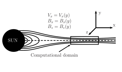
Figure 1: Model of the coronal streamer belt: a schematic view.

The magnetic and plasma flow configuration in a solar coronal streamer belt beyond its helmet cusp is characterized by a region of cospatial magnetic shear and a cross-stream velocity variation reminiscent of a ‘wake’ flow. Suitably simplified, a local study of streamer belt dynamics may then consider a ‘boxed’ model of a fluid wake – current sheet configuration as sketched in Fig. 1. A large number of previous studies have identified the various linear MHD instabilities supported by such an equilibrium configuration, with purely incompressible studies EinaudiBoncinelliDahlburgKarpen1999 , as well as extensions to the compressible regime DahlburgKeppensEinaudi2001 ; WangLeeWeiAkasofu1988 ; EinaudiChibbaroDahlburgVelli2001 ; DahlburgEinaudi1999 . Their applications cover a range of physical problems, as they are used to model dynamics at the heliospheric current sheet WangLeeWeiAkasofu1988 , mechanisms for variable slow solar wind formation and acceleration EinaudiBoncinelliDahlburgKarpen1999 , and plasmoid formation and evolution in the solar streamer belt EinaudiChibbaroDahlburgVelli2001 ; DahlburgKarpen1995 ; Einaudi1999 .

Similarly idealized configurations equally containing velocity shear layers co-spatial with an electric current sheet or neutral sheet have been used to investigate the linear and nonlinear stability properties of planar and non-planar current – vortex sheets Dahlburg1998 ; ShenLiu1999 ; DahlburgBoncinelliEinaudi1997 ; AntognettiEinaudiDahlburg2002 ; DahlburgEinaudi2001 ; DahlburgEinaudi2000 ; OfmanChenMorrisonSteinolfson1991 and planar magnetized jets Dahlburg1998 ; BiskampSchwarzZeiler1998 ; DahlburgKarpen1994 ; DahlburgBoncinelliEinaudi1998 ; OfmanChenMorrisonSteinolfson1991 . These configurations were investigated in the context of solar flares and surges, among other applications. The possibility of having both shear-flow related instabilities, and ideal and resistive magnetic instabilities, allow the plasma to transit to turbulent regimes via various routes in its further nonlinear evolution. Energy can be tapped from the background mean flow, with localized reconnection events releasing magnetic energy.

In this paper, we revisit the stability properties for a compressible wake – current sheet model of streamer belt dynamics, and extend earlier two-dimensional nonlinear simulations DahlburgKeppensEinaudi2001 ; EinaudiChibbaroDahlburgVelli2001 ; AntognettiEinaudiDahlburg2002 to three-dimensional MHD computations. The necessity to model the compressive aspects when applying the ‘box-model’ from Fig. 1 to encompass both the slow and fast solar wind regions is obvious since the wind becomes supersonic sufficiently close to the Sun (at roughly $5\,R_{\odot}$, as follows from Parker’s model Parker1958 ). Compressibility can give rise to new effects as compared to incompressible studies, such as nonlinear steepening of ideal sinuous instabilities under supersonic flow conditions to form fast magnetosonic shock fronts DahlburgKeppensEinaudi2001 ; AntognettiEinaudiDahlburg2002 , and the domination of fully three-dimensionally structured unstable modes over two-dimensional ones DahlburgEinaudi2000 ; DahlburgKeppensEinaudi2001 . In the incompressible case, the validity of Squires theorem DahlburgKarpen1995 precluded the latter possibility and allowed one to concentrate on 2D dynamics. It is the main result of this paper to show that (1) strongly supersonic magnetized wakes, characterized by a plasma beta of order unity, also have dominant 3D sinuous instabilities which (2) can lead to fully 3D structured fast magnetosonic shock fronts in their nonlinear evolution.

Earlier, formation and amplification of fast magnetosonic shocks was shown for supersonic super-Alfvénic wakes by means of numerical simulations DahlburgKeppensEinaudi2001 . These shocks were also observed in studies of 2D current-vortex sheets in the transonic regime AntognettiEinaudiDahlburg2002 . We supplement these earlier findings by a complete parametric study of initial state parameters which lead to shock formation. Our findings that dominant 3D sinuous instabilities are possible correct earlier claims to the contrary DahlburgKeppensEinaudi2001 where wavenumber space was not sufficiently explored. At the same time this calls for a study of the nonlinear development of a sinuous instability in three dimensions, which we perform as well.

It was pointed out by Wang et al. WangLeeWeiAkasofu1988 , on the basis of a linear stability analysis of a similar wake – current sheet configuration, that instabilities may develop in-situ at the heliospheric current sheet at radial distances of order 0.5 – 1.5 AU. They emphasized the importance of streaming sausage modes leading to traveling magnetic islands (clouds) and plasmoids. Our results focus on the streaming kink mode, and our nonlinear simulations demonstrate that it can lead to shock-dominated large-scale transients. This re-emphasizes the possibility that not all satellite solar wind observations of such events need to be directly mapped back to a specific solar coronal event (eruptive prominence or CME).

This paper is organized as follows. Section II presents the system of MHD equations describing the wake-current sheet evolution and the initial equilibrium configuration studied. Section III describes the numerical tools used for the linear stability analysis and for the nonlinear evolution studies. In Section IV, we present the linear stability analysis of the wake-current sheet configuration and identify the previously unexplored domain of the dominating three-dimensional sinuous instability. In Section V, the nonlinear MHD simulations with the Versatile Advection Code Toth1996 for different values of wake velocity contrast and magnetic field magnitude are discussed. Formation of fast magnetosonic shocks is demonstrated and their properties and generation conditions are described. Conclusions and a discussion of the relevance to in-situ streamer belt dynamics are placed in Section VI.

II MHD equations and equilibrium model

The system under consideration is described by the set of one-fluid compressible resistive MHD equations of the form:

$$\partial_{t}\rho+\nabla\cdot\left(\rho{\bf v}\right)=0,$$

$$\partial_{t}\left(\rho{\bf v}\right)+\nabla\cdot\left({\bf v}\rho{\bf v}-{\bf B}{\bf B}\right)+\nabla p_{tot}=0,$$

$$\partial_{t}e+\nabla\cdot\left({\bf v}e-{\bf BB}\cdot{\bf v}+{\bf v}p_{tot}\right)=\nabla\cdot\left({\bf B}\times\eta{\bf J}\right),$$

$$\partial_{t}{\bf B}+\nabla\cdot\left({\bf vB-Bv}\right)=-\nabla\times\left(\eta{\bf J}\right),$$

$${\bf J}=\nabla\times{\bf B},$$

$$p=\left(\gamma-1\right)\left(e-\rho v^{2}/2-B^{2}/2\right),\,\,p_{tot}=p+B^{2}/2,$$

where $\rho$ is the mass density, ${\bf v}$ is the plasma velocity, ${\bf B}$ is the magnetic field, and $e$ stands for total energy density. Other quantities are ${\bf J}$ – electric current, thermal pressure $p$ and the constants $\gamma\equiv 5/3$ – adiabatic index, and $\eta$ – resistivity coefficient. The resistive source terms are taken along to accurately simulate the small-scale reconnection events which only occur far into the nonlinear regime in the cases studied below.

Guided by the box model of Fig. 1, the magnetized wake flow co-spatial with the current sheet can be modeled as a force-free equilibrium configuration:

$$V_{x}=1-{\rm cosh}^{-1}y,\,\,V_{y}=0,\,\,V_{z}=0$$

$$B_{x}=M_{a}^{-1}{\rm tanh}\frac{y}{w},\,\,B_{y}=0,\,\,B_{z}=M_{a}^{-1}{\rm cosh}^{-1}\frac{y}{w}$$

$$\rho=1.0,\,\,p=(\gamma M_{s}^{2})^{-1},$$ (1)

where $M_{s}$ and $M_{a}$ are the sonic and Alfvénic Mach numbers for the fast flow streams, respectively, and $w$ describes the thickness of the current sheet relative to the width of the wake flow. The latter, together with the density and velocity of the fast flow streams, has been used to define our unit system. The plasma $\beta$ is then found from $\beta=(2M_{a}^{2})/(\gamma M_{s}^{2})$. If not mentioned otherwise, we set $w=1$. The same force-free equilibrium was analyzed in DahlburgKeppensEinaudi2001 , while a similar, but non force-free magnetic configuration, was used in WangLeeWeiAkasofu1988 .

III Numerical tools

Linear stability analysis of the wake-current sheet configuration was performed numerically with the LEDAFLOW code NijboerHolstPoedtsGoedbloed1997 . This code can compute the complete MHD spectrum of all waves and instabilities that are eigenfrequencies of one-dimensionally varying equilibria containing background plasma flows. The linearized MHD equations are discretized using finite elements (quadratic and cubic Hermite polynomials) in the direction of inhomogeneity and a Fourier representation of the perturbations in the invariant directions. Assuming a temporal variation as $\exp(\lambda\,t)$, application of the Galerkin procedure results in a complex non-Hermitian eigenvalue problem which is then solved by a complex QR-decomposition-based solver. For each isolated eigenvalue $\lambda$, the set of corresponding eigenfunctions can be found with an inverse vector iteration. In the QR mode, the whole spectrum for a given set of Fourier mode numbers is calculated, but the amount of grid points in the finite element representation is usually limited to 100 – 120 points. In inverse iteration mode, the spatial resolution is much higher to be able to get converged eigenfrequencies with strong gradients in their eigenfunctions (up to 5000 points). The boundary conditions implemented in LEDAFLOW assume perfectly conducting walls at $y$-boundaries, which is, strictly speaking, not applicable to the streamer belt configuration. To prevent any influence of these conducting walls on the solution of the eigenvalue problem, one should place them at sufficiently large distances in the perpendicular $y$-direction, and check whether the eigenfunctions are localized away from the computational domain boundaries and vanish close to the walls.

Nonlinear modeling of the wake-current sheet dynamics was performed by the general finite-volume-based Versatile Advection Code (VAC) Toth1996 ; Keppens2001 . For all runs we used the full set of compressible resistive MHD equations with a constant resistivity $\eta=10^{-4}$ value. The one-step total variation diminishing (TVD) method Harten1983JComputPhys was employed, which is a second-order accurate shock-capturing scheme. It uses an approximate Roe-type Roe1981 Riemann solver with the minmod (for 3D simulations) or Woodward (for 2.5D simulations) limiting applied to the characteristic waves.

The rectangular computational domain has periodic boundaries in the streamwise $x$-direction, and open boundaries in the cross-stream direction $y$, such that perturbations reaching these boundaries are allowed to propagate freely outside the computational box. For 3D runs, the spanwise direction $z$ is periodic as well. We used non-equidistant rectangular grids with a symmetric (around $y=0$) accumulation near the core of the wake. Grid resolutions varied from $100\times 200$ up to $300\times 600$ in 2.5D and from $60\times 90\times 60$ up to $100\times 150\times 100$ in 3D cases. The grid lengths in the streamwise and spanwise directions are found from $L_{x}=2\pi/k_{x}$ and $L_{z}=2\pi/k_{z}$, respectively, with wavenumbers $k_{x},\,k_{z}$ corresponding to the most unstable mode identified from the linear stability analysis. For the cross-stream boundary, the open boundaries are placed at $L_{y}=\pm 25$–$50$ depending on the localization of the unstable eigenmode. 2.5D runs were performed on an SGI Octane workstation, while 3D simulations were executed on typically 32 processors of the SGI Origin 3800 at the Dutch Supercomputing Centre, using openMP for parallelization purposes.

IV Linear stability analysis

Depending on the parameters of the one-dimensionally varying (but fully three-dimensionally structured) equilibrium configuration given by Eqs. (1), as well as on the value of the resistivity and the lenghtscales of the imposed perturbation, up to three different mode types may be destabilized in the wake-current sheet configuration. These are known as the ideal sinuous (or streaming kink) mode, and an ideal and a resistive varicose (sausage-type) mode Einaudi1999 ; WangLeeWeiAkasofu1988 . In a 2D case these types are easily distinguishable by the symmetry in their cross-stream velocity perturbations, which is even for the sinuous mode and odd for both varicose modes. In a 3D case these symmetry properties are broken. Here we shall mainly focus at the instability of an ideal sinuous type, already present in unmagnetized hydrodynamic wake configurations. In the range of Mach and Alfvén Mach numbers investigated, its growth rate is always larger than that of the varicose modes, and thus the sinuous mode is expected to dominate the evolution of the system. This mode is also known to demonstrate interesting nonlinear evolution: in 2.5D MHD simulations, sinuous mode instabilities led to the self-consistent formation of fast magnetosonic shocks in the nonlinear stage DahlburgKeppensEinaudi2001 .

In Fig. 2 a typical spectrum of a wake-current sheet system obtained with LEDAFLOW is presented. The parameters used are for a supersonic $M_{s}=3$, super-Alfvénic $M_{a}=5$ wake at fixed streamwise wavenumber $k_{x}=0.35$ and spanwise wavenumber $k_{z}=0.15$. The figure shows individual complex eigenfrequencies $\lambda$ throughout the complex plane, but for the value of the resistivity $\eta=0.01$, the ideal and resistive varicose instabilities are fully suppressed, and only the ideal sinuous mode remains unstable in the system (marked by the arrow in Fig. 2). Since the sinuous instability is ideal in nature, its growth rate does not depend on the value of the resistivity chosen. The eigenfunctions, namely the perturbed plasma density $\delta\rho$ and cross-stream velocity $\delta v_{y}$, for the unstable sinuous mode are shown in Fig. 3. The instability growth rate is $\gamma\approx 0.0402$ and the phase velocity $v_{ph}\approx 0.55$. It is seen that $\delta v_{y}$ is nearly symmetric (even) with respect to $y=0$, while the density perturbation has a more complicated structure but is in essence odd. All linear stability results following are performed for a fixed value of resistivity as used in the nonlinear simulations, namely $\eta=10^{-4}$.

The maximal sinuous mode growth rate is achieved for an incompressible (limit $M_{s}\rightarrow 0$), purely hydrodynamical (B=0) case. In incompressible magnetized wakes, the dominant instability was found to be two-dimensional having zero spanwise wavenumber, in agreement with the Squires theorem DahlburgKarpen1995 . When plasma compressibility is taken into account, as done in this paper, the situation can change drastically. In DahlburgKeppensEinaudi2001 , it was demonstrated that at high Mach numbers, an increase of the spanwise wavenumber can make the ideal compressible varicose mode more unstable. The sinuous mode growth rate, however, was believed to decrease with increasing $k_{z}$.

In Fig. 4, the numerically obtained growth rates for $M_{s}=3$, $M_{a}=5$ wakes of the ideal sinuous instability are plotted versus streamwise wavenumber $k_{x}$ (left panel A), and spanwise wavenumber $k_{z}$ (right panel B). The top curve in panel (A) for $k_{z}=0$ is identical to the corresponding dispersion curve for Mach 3 wakes shown in DahlburgKeppensEinaudi2001 , their Fig. 1(b). It is clearly seen from panel (A) that the region of destabilized $k_{x}$ is widest in the 2D case ($k_{z}=0$). Increasing the spanwise wavenumber $k_{z}$ leads to a shrinking of the instability domain from both sides, while for increasing $k_{z}$, the most unstable streamwise wavenumber also increases. This trend continues up to some upper value of $k_{z}>0.6$ where the sinuous mode becomes stable. Panel (B) demonstrates that the 2D landscape of growth rate versus streamwise $k_{x}$ and spanwise $k_{z}$ wavenumber, has a secondary ‘ridge’ which was overlooked in DahlburgKeppensEinaudi2001 . There, at a fixed wavenumber $k_{x}=0.55$, an increase of the spanwise wavenumber led to a decreasing growth rate for the sinuous mode (their Fig. 3(b)). Our panel (B) shows that their study overlooked the rather interesting case of larger streamwise wavelength (smaller $k_{x}$), where three-dimensional local extremum of growth rate was found for $k_{x}<0.25$. We can further observe that with an increase of the streamwise wavenumber $k_{x}$ from 0.075 up to values 0.35, both the growth rate and the instability existence domain (in $k_{z}$) increase, reaching their maximum values at $k_{x}\approx 0.35$, which corresponds to maximal 2D growth. Further increasing $k_{x}$ leads to a renewed drop in growth rate, however the instability domain does not change significantly. The latter can be seen when comparing our $k_{x}=0.35$ curve from panel (B) with the $k_{x}=0.55$ curve for Mach 3 wake flow in DahlburgKeppensEinaudi2001 , their Fig. 3(b). Below some $k_{x}<0.075$ the sinuous mode is fully stabilized again.

The importance of this secondary ridge in the growth rate landscape is marginal for the $M_{s}=3$, $M_{a}=5$ flow conditions of Fig. 4. Indeed, the absolute maximal growth rate corresponds to a purely 2D ($k_{z}=0$) mode with $k_{x}\approx 0.35$. However, for different combinations of Mach and Alfvén Mach number, the most unstable mode can be fully 3D in nature, a fact completely missed by earlier studies of this wake system. Variations of ideal sinuous mode maximal growth rate versus spanwise wavenumber for different values of $M_{s}$ and $M_{a}$ are plotted in Fig. 5, and the possibility of a 3D dominant instability is clearly manifested. Note that in this figure, the streamwise wavenumber $k_{x}$ varies from curve to curve, and has a value corresponding to the overall maximum in the growth rate landscape.

For a given Mach number, increasing the magnetic field strength (decrease of Alfvén Mach number $M_{a}$) acts to suppress the sinuous instability. This is also seen in Fig. 5, panel (A). The range of destabilized $k_{x}$ decreases, and the streamwise wavelength of the fastest growing mode decreases. When $M_{a}$ becomes smaller than some critical value $M_{a}^{cr}$, the system is stable. This critical value $M_{a}^{cr}$ was found to be approximately equal to 2.5, and this value is rather universal in a wide range of studied cases ($0<M_{s}<10$). This is consistent with DahlburgKeppensEinaudi2001 , their Fig. 2. Note that Wang et al. WangLeeWeiAkasofu1988 found a lower cut-off value (namely $M_{a}^{cr}\approx 1.2$) which must be due to the different equilibrium configuration used. Their equilibrium magnetic field strength is weaker at the center of the flow wake, while our configuration has a constant field magnitude throughout. Therefore, the stabilizing influence of magnetic tension translates into a lower cut-off value for $M_{a}^{cr}$.

Generally, with an increase of the sonic Mach number $M_{s}$, the overall maximal growth rate of the sinuous instability goes down, as well as the diapason of destabilized wavenumbers. For an Alfvén Mach number $M_{a}=3.5$, variations from Mach 2 till Mach 15 flows on the sinuous growth rates are shown in panel (B) from Fig. 5. Corresponding dependences ${\cal R}{\rm e}\left[\lambda(k_{x})\right]$ can be found elsewhere, e.g. see Fig. 1(b) in DahlburgKeppensEinaudi2001 .

The most important finding from Fig. 5 is that the most unstable sinuous mode may become oblique to the shear layer in a wake – current sheet system for sufficiently supersonic flows. Untill now, this was known for the compressible plane current-vortex sheet DahlburgEinaudi2000 as well as for varicose-type modes in compressible wake – current sheet configurations DahlburgKeppensEinaudi2001 . We found that for a given sonic Mach number larger than $M_{s}\approx 2.6$, there exists a range in $M_{a}$ where the maximum growth occurs for a mode with nonzero spanwise wavenumber. That diapason of $M_{a}$ for dominant three-dimensional instability is bounded from below and from above, and most wide near $M_{s}\approx 2.6$ where it is $2.9<M_{a}<4$. Its size decreases slowly with increasing $M_{s}$, so that even for highly supersonic wake flows the 3D instability domain is non-negligible, e.g. for $M_{s}=10$ it is found in the range $2.65<M_{a}<3.025$.

In the next sections we will study the nonlinear evolution of the wake–current sheet system in 2D and 3D using the information about the most unstable modes as calculated by LEDAFLOW for constructing the initial conditions.

V Nonlinear evolution and shock formation

V.1 2.5D MHD parameter study of shock formation

Since we are mainly interested in the nonlinear evolution of sinuous-type modes which have the largest growth rates and therefore dominate the system, the initial equilibrium configuration given by Eqs. (1) was perturbed by a symmetric cross-stream velocity perturbation of the form:

$$\delta v_{y}\sim\varepsilon\sin\left(k_{x}x\right)\exp(-y^{2}),$$

with typical values of $\varepsilon=10^{-3}..10^{-2}$. A comparative analysis of the nonlinear wake response to such perturbations in 2.5D MHD, for varying sonic and Alfvén Mach numbers, was presented in DahlburgKeppensEinaudi2001 . Here, we will focus on previously unaddressed issues, namely the interplay between simultaneously excited modes having different lenghtscales and growth rates, and the properties and formation conditions for shock waves, which are observed in the simulations at the instability saturation stage.

Mode-mode interplay

In Fig. 6, an example of a 2.5D MHD simulation is presented. By definition, all 2.5D simulations include only $k_{z}=0$ modes. Initially, two sinuous modes with streamwise wavenumbers $k_{x1}=0.35$ (mode 1) and $k_{x2}=0.35/3=0.11667$ (mode 2) were excited on the grid with amplitudes $\varepsilon_{1}=2.5\cdot 10^{-5}$ and $\varepsilon_{2}=10^{-2}$, respectively. For the simulated $M_{s}=3$, $M_{a}=5$ ($\beta=3.33$) wake, mode 1 corresponds to the dominant 2D fastest growing mode in the system. Note that we perturb the slower growing mode at a higher amplitude to force mode interaction. Fig. 6 shows snapshots of density and cross-stream velocity, while for the same time frames, Fig. 7 presents the spatial spectrum of the cross-stream velocity. This spatial Fourier transform performed for the sequence of snapshots allows to extract information on the linear growth rate for each mode and to confirm LEDAFLOW predictions. The linear results of the previous section were found to be very accurate, the difference in growth rates deduced from VAC simulations and those obtained by LEDAFLOW is usually less than 1%.

At early times, mode 2 is seen to grow with the growth rate $\approx 0.018$. However, at times around $T=200$, as it is clearly seen in the spectral evolution, mode 1 obtains a comparable amplitude. Having the larger growth rate, mode 1 develops faster, and at times around $T=250$ its amplitude becomes larger than that of mode 2. Later on in the nonlinear evolution the short-wavelength mode 1 remains the most dominant one, but a cascade to smaller wavelength dynamics is obviously occuring. Note that initially (times $T<200$) this only involves direct overtones of the two excited modes.

Similar observations can be made as follows. In the linear stage of the instability, the volume average cross-stream kinetic energy in the system plotted in Fig. 8, and defined as

$$E^{y}_{Kin}=\left(2L_{x}L_{y}L_{z}\right)^{-1}\int_{0}^{L_{x}}\int_{-0.5L_{y}}^{0.5L_{y}}\int_{0}^{L_{z}}\rho v_{y}^{2}dxdydz,$$ (2)

grows exponentially in accordance with the slower growing mode 2. Again, its slope changes near $T=200$ indicating that the faster growing mode 1 comes into play. Eventually, transverse kinetic energy growth is halted and this saturation point typically coincides with the time where the largest density contrast is achieved. The total kinetic energy of the system decreases, while the magnetic energy increases indicative of the occuring energy conversion processes.

Tresholds for shock formation

Depending on the system parameters, exactly at the point of maximal density contrast, shock waves may be formed. They are clearly detected in the density snapshot at time $T=300$ from Fig. 6. Note that these shocks extend far out into the fast stream regions, up to 25 wake widths in the cross-stream direction. Fig. 9 shows a cross-cut of the density variation at this time, taken at about 10 wake widths above the wake-current sheet. The shocks carry strong density contrasts, up to a factor of 2. Note that due to the mode-mode interaction, successive shock fronts can have different strengths, and their interseparation no longer corresponds to the wavelength of the linearly most unstable mode. This cross-cut can loosely be interpreted as a time-evolution of an in-situ satellite measurement, since the shock fronts are typically advected over the periodic side boundaries for more than a full advection cycle.

To identify the type of the shock front, we used Rankine-Hugoniot relations to determine the shock speed. This is most easily found from mass continuity, where the velocity of the shocks is found as $V_{sh}=(\left(\rho v_{\perp}\right)^{before}-\left(\rho v_{\perp}\right)^{after})/(\rho^{before}-\rho^{after})$. The shock type then follows from determining Alfvén, slow- and fast magnetosonic Mach number transitions in the coordinate system which moves with the shock velocity. Shock waves formed at the nonlinear stage of the sinuous instability of a supersonic magnetized wake were found to be fast magnetosonic in nature.

The steepening of the sinuous wave fronts into shock waves is possible only above a threshold value of sonic Mach number. That threshold depends on the amplitude of the magnetic field (hence on $M_{a}$). In a pure hydrodynamical case ($M_{a}=\infty$), sonic shocks are formed for supersonic wake flows with $M_{s}\geq 2.10$. Shocks appeared for all studied hydrodynamic cases in the range $2.10<M_{s}<10.0$ and no upper limit of $M_{s}$ for their formation was found. This hydro critical value is recovered in weak ($M_{a}>5$) magnetized wakes. However, with an increase of the magnetic field magnitude, the minimum value $M_{s}^{Min}$ of the sonic Mach number needed for shock formation, is increased. This is presented in Fig. 10, where threshold sonic Mach numbers are plotted versus the Alfvén Mach numbers. Formation of the shock fronts was shown to be possible for any $M_{a}$ where the sinuous mode is still unstable ($M_{a}>2.5$). Hence, for any magnetic field strength, where the sinuous instability is not suppressed linearly, we were able to identify a shock-treshold value of Mach number $M_{s}^{Min}$. For all $M_{s}>M_{s}^{Min}(M_{a})$ shock fronts form self-consistently through wave front steepening.

Most of the nonlinear runs to determine the parameter ranges for shock formation were performed for systems of length $L_{x}=2\pi/k_{x}^{m}$, with $k_{x}^{m}$ being the streamwise wavenumber of the fastest growing mode. It turns out that shocks can appear having different scales in the x-direction, since there exists a diapason of streamwise wavenumbers $k_{x}$, located around $k_{x}^{m}$, for which shocks develop. At scales sufficiently far from $k_{x}^{m}$, formation of shock waves was not observed. For a given Alfvén Mach number, with an increase of the wake speed contrast ($M_{s}$), the angle between the shock front and the streamwise direction decreases. Hence the density perturbations become more and more cuddled up to the core of the wake, and thus not always reach far cross-stream regions.

Finally, when applied to the coronal streamer belt, the width of the current sheet – $w$ in Eqs. (1) – is typically much smaller than that of the fluid wake EinaudiChibbaroDahlburgVelli2001 . With a decrease of the relative width of the current sheet, the number of grid points needed to achieve acceptable resolutions grows rapidly, and simulations become more and more time- and memory consuming. Nevertheless, for selected cases we did vary the current sheet width, and these experiments did not show any qualitative difference in the nonlinear stage of evolution, indicating that the model of equal-sized wake and current sheet used throughout this paper is warranted. Quantitatively, as can also be obtained from a linear LEDAFLOW analysis, the growth rate and streamwise wavenumber of the most unstable sinuous mode decreases when the current sheet width goes down.

V.2 Case studies in 3D MHD

The 2.5D simulations in the previous section excluded the emergence of fully 3D structured shock fronts. However, our linear stability study demonstrated the existence of dominant 3D unstable modes. Here we discuss three particular three-dimensional runs performed for different parameters of the equilibrium configuration and for different initial excitations. We investigate two distinct cases: (1) a wake with a dominant purely 2D mode, where we look into the possibility of 3D shock structuring due to mode-mode interactions; and (2) a wake previously identified to have a dominant 3D linear mode.

Mode-mode interaction

In Fig. 11, plasma density isosurfaces are plotted for different stages in the sinuous mode instability development. In the first column of Fig. 11, values of sonic and Alfvén Mach numbers were chosen to be $M_{s}=3$, $M_{a}=5$, as in the 2.5D run from Fig. 6. The wake was perturbed with two modes: a pure 2D mode – the most dominant instability – having $k_{x}=0.35,\,\,k_{z}=0$, and a 3D mode $k_{x}=0.35/3=0.11667,\,\,k_{z}=0.125$. The amplitude of the 3D mode ($10^{-2}$) was much larger than that of the 2D mode ($10^{-5}$). At first, the 3D sinuous instability develops in accordance with its growth rate $\approx 0.018$, and the emerging density structure is clearly three-dimensional. However at times around $T\approx 175$ (middle snaphot), the 2D mode comes into play. It leads to elongation of the density structures along the $z$-axis. It again causes a slope change in the $E^{y}_{kin}(t)$ dependence plotted in Fig. 12. This continues untill the wake density structure tends to be mainly two-dimensional, with very slight modulations along the $z$-axis. In particular, the emerging shocks are nearly plane-parallel, as in the 2.5D simulations.

If the same system is initially perturbed by the 3D mode alone, as is done in the middle column in Fig. 11, one can obtain fully 3D structured shock-dominated wake dynamics. The two-dimensional mode starts to grow from the noise level in this case, and obtains noticeable amplitude only at times when the 3D instability is close to saturation. The shock fronts have a truly 3D topology. Note that at times around $T=250$ each high density blob splits into parts whose scale corresponds to the scale of the fastly growing 2D $k_{x}=0.35,\,\,k_{z}=0$ mode. After saturation, a set of nearly two-dimensional (as seen from the third snapshot in the middle column in Fig. 11) structures form. The number of structures corresponds to the scale of the initially excited 3D mode, but their size in the streamwise direction is strongly influenced by the $k_{x}=0.35,\,\,k_{z}=0$ mode. These two runs demonstrate that 3D shock structuring can even emerge from wakes with dominant 2D linear instabilities, but only under rather selective initial excitations.

Dominant 3D instability

The last column in Fig. 11 shows the nonlinear evolution of the density in pure three-dimensional dynamics of the sinuous instability for the case $M_{s}=3$, $M_{a}=3.5$ ($\beta=1.6$). Above, it was demonstrated that for these parameters, the most unstable sinuous mode is oblique to the wake’s core and has the wavenumbers $k_{x}=0.375,\,\,k_{z}=0.15$ (see Fig. 5). Note how at all stages in the evolution, the spatial density distribution remains fully 3D. As compared to the other cases shown, the maximal density contrast reached in the nonlinear stages is larger. For these parameters, the fast magnetosonic shock fronts emerging in the nonlinear stage have a fairly complex 3D structure. The transverse kinetic energy evolution is plotted in Fig. 12.

VI Conclusions

In this paper we performed a numerical study of the linear properties and nonlinear evolution of wake – current sheet configurations by means of compressible resistive MHD simulations. We focused on three-dimensional effects for the ideal sinuous-type instability. In contrast to previous studies, we have shown that there exist ranges of Mach number $M_{s}$ and Alfvén Mach number $M_{a}$, where the most unstable sinuous mode is oblique to the shear layer. Such pure three-dimensional instabilities develop nonlinearly into fully 3D deformations of the wake system containing fast magnetosonic shock fronts. For dominant 3D instabilities, the Mach number should exceed a threshold value $M_{s}>2.6$. With increase of $M_{s}$, the range of $M_{a}$ corresponding to 3D instability decreases, but even for highly supersonic cases, a dominant 3D instability still exists in some range of $M_{a}$. At the nonlinear stage of this sinuous instability in the supersonic regime, self-consistent formation of fast magnetosonic shocks is observed. They carry density jumps (by factors of 2) in cross-stream fast flow regions far away from the wake center. As a result of mode-mode interaction, the shock strengths and interseparations can vary. Depending on the wake velocity contrast and magnetic field magnitude, as well as on the streamwise and spanwise scale of the initial perturbation, these shocks may have plane-parallel as well as complicated three-dimensional structure. Shock fronts appear only for Mach numbers above some critical value, which depends on magnetic field strength, but is always larger than the hydro limit $M_{s}=2.1$.

Finally, let us estimate the heliospheric regions, where our box-model predicts the possibility for in-situ compressible transients. Using the Parker model Parker1958 for the interplanetary magnetic field one finds, in a manner originally done by Wang et al. WangLeeWeiAkasofu1988 , Alfvén and sonic Mach number radial dependencies of the form:

$$M_{s}(r)=\frac{\delta v(r)}{v_{a}^{0}}\sqrt{\frac{2}{\gamma\beta_{0}}}\sqrt[4]{\frac{r^{2}}{r^{2}+1}},$$

$$M_{a}(r)=\frac{\delta v(r)}{v_{a}^{0}}\sqrt{\frac{2r^{2}}{r^{2}+1}},$$

where $\delta v(r)$ is the velocity contrast between fast and slow wind streams, and $\beta_{0}$ and $v_{a}^{0}$ indicate the plasma beta and Alfvén speed at 1 AU. For solar wind parameters at the Earth’s orbit given by $n=5$ cm^-3, $B=5$nT, $T_{e}=2\cdot 10^{5}$K, $T_{p}=4\cdot 10^{4}$K (taken from Winterhalter1994 ), one finds $\beta_{0}\approx 1.6$, while $v_{a}^{0}\approx 50$ km/sec. Assuming that the fast-slow solar wind velocity contrast, as determined by Ulysses measurements McComas1998 to be of the order $\delta v\approx 350$km/sec, does not change significantly with radius beyond the various magnetosonic transitions, one can compute $M_{s}(r)$ and $M_{a}(r)$ dependencies.

Our linear theory predicted that the sinuous mode is destabilized for $M_{a}\geq 2.5$ which then corresponds to distances beyond 0.3 AU from the Sun. Relevant heliospheric distances turn out to be 0.3 AU – 1.5 AU. Since we used the fluid wake scale length and the fast-slow velocity contrast to define dimensionless variables, we can verify whether the instability grows sufficiently fast to influence conditions at 1 AU. The flow wake width is observationally determined to be of order 300.000km at 1 AU, while at a heliospheric distance of order 0.5 AU it is estimated to be around 150.000km Winterhalter1994 . Our time unit will then correspond to approximately 7 minutes. At 0.5 AU, the most unstable sinuous mode has a dimensionless growth rate of 0.0272 and corresponding streamwise wavenumber of $k_{x}=0.325$. Hence, the sinuous instability could fully develop within about 25 hours, in close correspondence with the transit time to 1 AU. The lengthscale of these compressive perturbations are then of order $2\cdot 10^{-2}$AU. This points to the distinct possibility of in-situ shock formation at wake-current sheet configurations within the heliosphere.

Acknowledgements. This work was performed as part of the Computational Science programme   ”Rapid Changes in Complex Flows” coordinated by JPG, and funded by the Netherlands Organization for Scientific Research (NWO). Computing facilities were provided by NCF (Stichting Nationale Computerfaciliteiten). RK and JPG performed this work supported by the European Communities under the contract of Association between EURATOM/FOM, carried out within the framework of the European Fusion Programme. Views and opinions expressed herein do not necessarily reflect those of the European Commission.

Figure 2: MHD spectrum of a compressible wake-current sheet with $M_{s}=3$, $M_{a}=5$, $k_{x}=0.35$, $k_{z}=0.15$, $\eta=0.01$. The unstable sinuous mode is marked.

Figure 3: Eigenfunctions corresponding to the unstable sinuous mode from Fig. 2. Real and imaginary parts of the cross-stream perturbed velocity and perturbed density are shown.

Figure 4: Ideal sinuous mode growth rate versus streamwise wavenumber $k_{x}$ and spanwise wavenumber $k_{z}$. (A) At fixed spanwise wavenumber $k_{z}=\{0.0,0.25,0.5,0.6\}$ top to bottom. (B) At fixed streamwise wavenumber $k_{x}=\{0.35,0.25,0.15,0.11667,0.1,0.075\}$ top to bottom.

Figure 5: Maximum growth rates of the ideal sinuous mode in a wake – current sheet system versus spanwise wavenumber for different $M_{s}$ and $M_{a}$. Note that the streamwise wavenumber $k_{x}$ varies from curve to curve. (A) At fixed $M_{s}=3$, curves corresponding to $M_{a}=\{5.0,4.5,4.0,3.5,3.25,3.0,2.9,2.8\}$ top to bottom, (B) At fixed $M_{a}=3.5$, curves corresponding to $M_{s}=\{2.0,2.5,3.5,4.0,5.0,15.0\}$ top to bottom.

Figure 6: 2.5D MHD simulations of a wake-current sheet configuration with $M_{s}=3$, $M_{a}=5$, $\eta=10^{-4}$. Plasma density (left panels) and cross-stream velocity (right panels) at times $T={100,175,200,250,300,500}$. Two sinuous modes were excited and shocks of different strengths emerge at $T=300$.

Figure 7: Fourier spectrum of cross-stream velocity corresponding to the 2.5D run from Fig. 6.

Figure 8: Vertical kinetic energy, total kinetic energy and magnetic energy versus time for the 2.5D run from Fig. 6.

Figure 9: Plasma density distribution along the streamwise direction, far into the fast stream regions ($y=10.1$) at $T=300$, as obtained from Fig. 6. The fast shocks carry density jumps up to factors of two.

Figure 10: Threshold value of sonic Mach number necessary for shock formation versus Alfvén Mach number.

Figure 11: 3D MHD simulations of wake-current sheets. First column: $M_{s}=3$, $M_{a}=5$, two modes excited: $(k_{x}=0.35,\,\,k_{z}=0)$ and $(k_{x}=0.35/3=0.11667,\,\,k_{z}=0.125)$. Second column: as in first column, only the 3D mode excited initially. Third column: $M_{s}=3$, $M_{a}=3.5$, initiated with its dominant three-dimensional sinuous mode $(k_{x}=0.375,\,\,k_{z}=0.15)$. Density isosurfaces at consecutive times (top to bottom) are shown.

Figure 12: Evolution of vertical kinetic energies for all three 3D runs in Fig. 11.

References

- [1] G. Einaudi, P. Boncinelli, R. Dahlburg, J. Karpen. Formation of a slow solar wind in a coronal streamer. Journal of Geophysical Research, 104(A1):521–534, 1999.
- [2] R.B. Dahlburg, R. Keppens, G. Einaudi. The compressible evolution of the super-Alfvénic magnetized wake. Physics of Plasmas, 8(5):1697–1706, 2001.
- [3] S. Wang, L. C. Lee, C. Q. Wei, and S.-I. Akasofu. A mechanism for the formation of plasmoids and kink waves in the heliospheric current sheet. Solar Physics, 117:157–169, 1988.
- [4] G. Einaudi, S. Chibbaro, R. Dahlburg, M. Velli. Plasmoid formation and acceleration in the solar streamer belt. The Astrophysical Journal, 574:1167–1177, 2001.
- [5] R.B. Dahlburg, G. Einaudi. Compressible aspects of slow solar wind formation. Space Science Reviews, 87(1):157–160, 1999.
- [6] R.B. Dahlburg, J.T. Karpen. A triple current sheet model for adjoining coronal helmet streamers. Journal of Geophysical Research, 100(A12):23489–23497, 1995.
- [7] G. Einaudi. Nonlinear evolution of magnetic and Kelvin-Helmholtz instabilities in the solar corona. Plasma Physics and Controlled Fusion, 41:A293–A305, 1999.
- [8] R.B. Dahlburg. On the nonlinear mechanics of magnetohydrodynamic stability. Physics of Plasmas, 5(1):133–139, 1998.
- [9] C. Shen, Z.X. Liu. The coupling mode between Kelvin-Helmholtz and resistive instabilities in compressible plasmas. Physics of Plasmas, 6(7):2883–2886, 1999.
- [10] R.B. Dahlburg, P. Boncinelli, G. Einaudi. The evolution of plane current-vortex sheets. Physics of Plasmas, 4(5):1213–1226, 1997.
- [11] A. Antognetti, G. Einaudi, R.B. Dahlburg. Transonic and subsonic dynamics of current-vortex sheet. Physics of Plasmas, 9(5):1575–1583, 2002.
- [12] R.B. Dahlburg, G. Einaudi. Three-dimensional secondary instability in plane current-vortex sheets. Physics of Plasmas, 8(6):2700–2706, 2001.
- [13] R.B. Dahlburg, G. Einaudi. The compressible plane current-vortex sheet. Physics of Plasmas, 7(5):1356–1365, 2000.
- [14] L. Ofman, X. L. Chen, P. J. Morrison, and R. S. Steinolfson. Resistive tearing mode instability with shear flow and viscosity. Physics of Fluids B, 3:1364–1373, 1991.
- [15] D. Biskamp, E. Schwarz, and A. Zeiler. Instability of a magnetized plasma jet. Physics of Plasmas, 5:2485–2488, July 1998.
- [16] R.B. Dahlburg, J.T. Karpen. Transition to turbulence in solar surges. The Astrophysical Journal, 434:766–772, 1994.
- [17] R.B. Dahlburg, P. Boncinelli, G. Einaudi. The evolution of a plane jet in the neutral sheet. Physics of Plasmas, 5(1):79–93, 1998.
- [18] E. N. Parker. Dynamics of the Interplanetary Gas and Magnetic Fields. The Astrophysical Journal, 128:664–676, 1958.
- [19] G. Tóth. A general code for modeling MHD flows on parallel computers: Versatile Advection Code. Astrophysical Letters and Communications, 34:245, 1996.
- [20] R.J. Nijboer, B.v.d. Holst, S. Poedts, J.P. Goedbloed. Calculating magnetohydrodynamic flow spectra. Computer Physics Communications, 106(1-2):39–52, 1997.
- [21] R. Keppens. Dynamics controlled by magnetic field: parallel astrophysical computations. Parallel Computational Fluid Dynamics - Trends and Applications, edited by C.B. Jenssen et al, pages 31–42, 2001.
- [22] A. Harten. On the symmetric form of systems of conservation laws with entropy. Journal of Computational Physics, 49:151–164, January 1983.
- [23] P.L. Roe. Approximate Riemann solvers, parameter vectors, and difference schemes. Journal of Computational Physics, 43:357–372, 1981.
- [24] D. Winterhalter, E. J. Smith, M. E. Burton, N. Murphy, and D. J. McComas. The heliospheric plasma sheet. Journal of Geophysical Research, 99:6667–6680, April 1994.
- [25] D. J. McComas, S. J. Bame, B. L. Barraclough, W. C. Feldman, H. O. Funsten, J. T. Gosling, P. Riley, R. Skoug, A. Balogh, R. Forsyth, B. E. Goldstein, and M. Neugebauer. Ulysses’ return to the slow solar wind. Geophysical Research Letters, 25:1–4, 1998.