The Absorption Signatures of Dwarf Galaxies: The $z=1.04$ Multi–cloud Weak Mgii Absorber Toward PG 1634+706:

Abstract

We analyze high resolution spectra of a multi–cloud weak [defined as $W_{r}({\hbox{{\rm Mg}\kern 1.00006pt{\sc ii}}})<0.3$ Å] absorbing system along the line of sight to PG $1634+706$. This system gives rise to a partial Lyman limit break and absorption in Mgii, Siii, Cii, Siiii, Siiv, Civ, and Ovi. The lower ionization transitions arise in two kinematic subsystems with a separation of $\simeq 150$ km s^-1. Each subsystem is resolved into several narrow components, having Doppler widths of $3$–$10$ km s^-1. For both subsystems, the Ovi absorption arises in a separate higher ionization phase, in regions dominated by bulk motions in the range of $30$–$40$ km s^-1. The two Ovi absorption profiles are kinematically offset by $\simeq 50$ km s^-1 with respect to each of the two lower ionization subsystem. In the stronger subsystem, the Siiii absorption is strong with a distinctive, smooth profile shape and may partially arise in shock heated gas. Moreover, the kinematic substructure of Siiv traces that of the lower ionization Mgii, but may be offset by $\simeq 3$ km s^-1.

Based upon photoionization models, constrained by the partial Lyman limit break, we infer a low metallicity of $\sim 0.03$ solar for the low ionization gas in both subsystems. The broader Ovi phases have a somewhat higher metallicity, and they are consistent with photoionization; the profiles are not broad enough to imply production of Ovi through collisional ionization. Various models, including outer disks, dwarf galaxies, and superwinds, are discussed to account for the phase structure, metallicity, and kinematics of this absorption system. We favor an interpretation in which the two subsystems are produced by condensed clouds far out in the opposite extremes of a multi–layer dwarf galaxy superwind.

1 Introduction

Quasar absorption line systems, as traced by their Mgii, provide a unique way to study our universe. Current classifications schemes for systems with detected Mgii file them into three main categories: those that are characterized by their strong Mgii absorption, those that reveal weak, narrow, single–cloud Mgii profiles, and those that exhibit weak, multiple cloud Mgii absorption. In this paper we analyze in detail the absorption profiles from a particular multiple cloud weak Mgii absorber at $z=1.04$ along the line of sight toward PG $1634+706$. The longer–term goal of a collection of similar studies will be to understand the relationships between the different classes of absorption systems, and the connections with the different types of galaxies and structures at various redshifts.

Although there are no distinct divisions between the three categories of Mgii absorption systems, by their properties they appear to be related to three different types of gaseous structures at $z\sim 1$. Strong Mgii absorbers [those with $W_{r}(2796)>0.3$ Å] show Lyman limit breaks and contain multiple clouds spread over tens to hundreds of kilometers per second (Churchill et al., 2000). A large majority of these absorbers are known to be associated with luminous galaxies ($>0.05L^{*}$, where $L^{*}$ is the Schechter luminosity), within an impact parameter of $40h^{-1}$ kpc of the quasar (Bergeron & Boissé, 1991; Bergeron et al., 1992; Le Brun et al., 1993; Steidel, Dickinson, & Persson, 1994; Steidel, 1995; Steidel et al., 1997). All of the strong Mgii absorbers ($dN/dz=0.91\pm 0.1$ at $<z>=0.9$ (Steidel & Sargent, 1992)) can be accounted for by regions of this size around the known population of luminous galaxies. The strong Mgii absorber spectral profiles, in chemical transitions of low and high ionization states, generally require multiple phases of gas, i.e. regions of differing densities that are spatially distinct (e.g. (Ding et al., 2003a, b)). The kinematics of the low ionization gas is generally consistent with what one would expect from the combined disks and halos of galaxies of a variety of morphological types (Charlton & Churchill, 1998; Steidel et al., 2002).

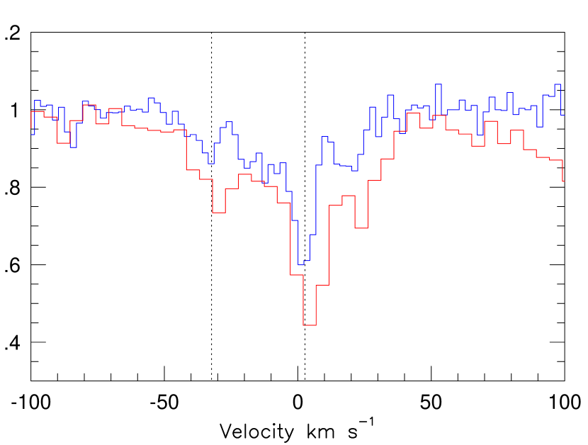
Figure 2: The Mgii $\lambda 2796$ from HIRES/Keck and the Siiv $\lambda 1394$ profile from STIS/HST are superimposed in velocity space, the weaker profile corresponding to Mgii. Although Mgii and Siiv appears to have similar structure, they appear to be offset by a few km s^-1. Vertical lines are drawn through the apparent centroid of two of the components in the Mgii profile.

In contrast to the strong Mgii absorbers, the single–component systems with weaker Mgii (rest frame equivalent widths $W(2796)<0.3$ Å) are typically not known to be directly associated with luminous galaxies (i.e. they are not within $50$–$100$ kpc of $>0.05L^{*}$ galaxies) (Churchill et al., 1999). These single–component weak Mgii systems have a significant absorption cross-section, with $dN/dz=1.10\pm 0.06$ for $0.02<W<0.3$ Å at $0.4<z<1.0$ (Churchill et al., 1999), similar to the value for all strong Mgii absorbers. The distribution of the number of Voigt profile components used to fit Mgii absorption systems is roughly Gaussian with a median of seven components. However, there is a strong excess of single cloud components relative to the rest of the distribution (see Fig. 2 in Rigby et al. (2002) and Table 7 of Churchill & Vogt (2001)). This implies that the single–component weak Mgii absorbers are primarily produced by a different class of object than the strong Mgii absorbers. Consistent with this interpretation, most of the single–component weak Mgii absorbers do not produce Lyman limit breaks (Churchill et al., 2000). Their Mgii profiles are generally quite narrow, with Doppler parameters of $b\sim 2$ – $5$ km s^-1. Their Civ profiles are broader and require a separate, higher ionization, phase of gas. Their low ionization phases are inferred to have metallicities greater than a tenth solar and to have sizes less than $\sim 10$–$100$ pc (Rigby et al., 2002; Charlton et al., 2003). The general properties of the single–cloud weak Mgii absorbers suggest an origin in some type of faded early extragalactic star cluster or in metal–rich fragments in cold dark matter mini–halos ”failed galaxies” (Rigby et al., 2002).

The third category of Mgii systems is characterized by multiple, weak components spread over tens of kilometers per second. About one third of the weak Mgii absorbers are in this category (Churchill et al., 1999). By definition, these are “weak Mgii absorbers”, since the total rest frame equivalent width of Mgii 2796 is $<0.3$ Å. Unlike the the strong Mgii absorbers, little is directly known about the environments of the multiple–component weak Mgii systems. However, the multiple–component weak category appears consistent with an extension of the distribution of the numbers of components fit to strong Mgii absorbers (see Fig. 2 in Rigby et al. (2002)). The weakness and kinematics of the multiple–component weak Mgii profiles might suggest a line of sight through the outer regions of a galaxy where the gas could be more diffuse and less dense. It is also possible that a dwarf galaxy, or even a low–metallicity giant galaxy would give rise to such weak Mgii absorption.

In this paper, we study a multiple–component, weak Mgii [rest frame equivalent width, $W_{r}(2796)=0.097\pm 0.008$ Å] absorber at $z\sim 1$. This absorber was modeled previously by Charlton et al. (2000), using low–resolution FOS/HST data along with the high–resolution Mgii profiles from HIRES/Keck. They determined that the Mgii clouds have a relatively low metallicity of $0.03$ solar, based on a comparison to a partial Lyman limit break. The Civ, detected in the FOS spectrum, was clearly offset from the low ionization clouds. This required an additional high ionization cloud producing absorption $\sim 200$ km s^-1 to the blue of the detected Mgii clouds. Charlton et al. (2000) predicted that this cloud should produce observable Cii, Siiii, and Siiv in the high resolution STIS spectrum. However, with just the low–resolution UV spectrum, they were unable to determine if the Civ detected at the same velocity as Mgii could arise in the same phase of gas with the Mgii, or if a separate phase would be needed. Also, the ionization conditions and metallicities of the high ionization clouds could not be well–constrained.

STIS/HST spectra of PG $1634+706$ are now available, with high resolution coverage of Ly$\alpha$ and the Lyman series, Siii, Siiii, Cii, Siiv, and Ovi. With these new data, we aim to test the models of Charlton et al. (2000), and to reach more detailed conclusions about the phase structure, metallicity, ionization conditions and kinematic properties of the $z=1.04$ system toward PG $1634+706$.

In § 2 we describe the spectra of quasar PG $1634+706$ used in our analysis, obtained with STIS/HST, FOS/HST and HIRES/Keck. We then present the data for the $z=1.04$ system along this line of sight in § 3 and make a qualitative comparison of the individual chemical transitions. Our analysis method, considering photoionization and collisional ionization models, is outlined in § 4. In § 5 we present results from modeling of this system and we summarize the conclusions in § 6. In § 7, we discuss possible scenarios for the origin of the $z=1.04$ system and the general implications for the nature of multiple–component, weak Mgii absorbers.

2 Data

Spectra of the $z=1.36$ quasar PG $1634+706$, obtained with the three instruments HIRES/Keck, STIS/HST, and FOS/HST, were used to study the various transitions from an intervening absorber at $z=1.0414$. Other Mgii systems along this line of sight are published elsewhere. There are three weak, single–cloud Mgii absorbers at $z=0.6540$, $z=0.8181$ and $z=0.9056$ (Churchill et al., 1999; Rigby et al., 2002; Charlton et al., 2003) and a strong Mgii absorber at $z=0.9902$ (Churchill & Vogt, 2001; Ding et al., 2003a).

Although a WFPC2/HST image of the quasar field exists, it is not deep, so it provides only a limited constraint on the luminosity of the host galaxy of this $z=1.04$ absorber. After subtraction of the point spread function of the $V=14.9$ quasar from the image, Farrah et al. (2002) did not detect any galaxies within the $\sim 36\arcsec$ Planetary Camera field of view to a magnitude of $m_{I}=22.5$ (at the $3\sigma$ level). This implies that there are no galaxies brighter than $\sim 0.5L^{*}$ with impact parameter less than $\sim 500$ kpc at the redshift of our absorber (Farrah et al. (2002) used $h=0.65$). Due to uncertainties in the PSF the limit is not as restrictive within $1-2$ kpc. Since even strong Mgii absorbers are associated with galaxies with luminosities as small as $0.05L^{*}$, this image does not allow us to usefully constrain the host galaxy properties for this or any of the other Mgii systems along the line of sight.

2.1 The HIRES Spectra

HIRES/Keck (Vogt et al., 1994) spectra at $R\sim 45,000$ (FWHM$\sim 6.6$ km s^-1) were obtained on 1995 July 4 and 5. The wavelength coverage is $3723$ to $6186$ Å. The typical signal-to-noise ratio per resolution element is $50$. The transitions we study here are Mgii $\lambda\lambda 2796,2803$ and Feii $\lambda 2600$. Churchill & Vogt (2001) describe the data reduction, continuum fitting, and Voigt profile fitting. We adopt the column densities and Doppler parameters presented in Charlton et al. (2000).

2.2 The STIS Spectra

Archival STIS/HST (Kimble et al., 1998) spectra were used to study Ly$\alpha$, Ly$\beta$, Ly$\gamma$, Ly$\delta$, Ly$8$, Cii $\lambda 1334$, Siii $\lambda 1260$, Siiii $\lambda 1206$, Siiv $\lambda\lambda 1393,1402$, Nv $\lambda\lambda 1239,1243$, and Ovi $\lambda\lambda 1032,1038$. Two data sets were obtained with different tilts of the E230M grating with an aperture of $0.2$ x $0.2$ ($R=30,000$, FWHM$\sim 10$ km s^-1). The first was obtained by Jannuzi et al. (proposal identification 8312, wavelength range of 2303 to 3111 Å) and the second by Burles et al. (proposal identification 7292, wavelength range from $1865$ to $2673$ Å). A third data set was obtained by Burles et al. (wavelength coverage $1830$ to $1870$ Å) with the $52$ x $0.02$ aperture of the G230M grating ($R=10,000$, FWHM$\sim 30$ km s^-1). We used this spectrum to study the higher order transitions of the Lyman series and the Lyman limit break. The reduction and calibration of all STIS data were performed using the standard STIS pipeline (Brown et al., 2002). Continuum fitting was performed using the techniques described in Churchill & Vogt (2001). We co-added the E230M spectra in cases of duplicate wavelength coverage to obtain higher signal-to-noise ratios (per resolution element) ranging from $8$ to $30$. We have verified that wavelength calibration is consistent between the STIS and HIRES datasets by comparing Mgii $\lambda\lambda 2796,2803$, Siii 1260 and Cii 1335 in the three single component, low ionization absorption systems found along this same line of sight (Charlton et al., 2003).

2.3 The FOS Spectra

FOS/HST data, with lower resolution ($R=1300$) and wavelength coverage $2225$ Å to $3280$ Å (G270H grating), were obtained as part of the Quasar Absorption Line Key Project (Bahcall et al., 1993, 1996; Jannuzi et al., 1998). These data were only used to study the Civ $\lambda\lambda 1548,1550$ absorption, since all other transitions had higher resolution coverage from STIS.

3 The $z=1.0414$ System

Figure 1 presents the absorption profiles of selected transitions for the $z=1.04$ absorber. These transitions are Ly$\alpha$, Mgii $\lambda\lambda 2796,2803$, Cii $\lambda 1335$, Siii $\lambda 1260$, Siiii $\lambda 1207$ Siiv $\lambda\lambda 1393,1402$, and Ovi $\lambda\lambda 1032,1038$. Also, Civ $\lambda\lambda 1548,1550$, covered in the lower resolution FOS spectrum, is shown. The region of the spectrum that provides a limit on Nv $\lambda 1239$ and Feii $\lambda 2600$ is also shown. The rest-frame velocities are aligned with the Mgii $\lambda 2796$ transition, where $v=0$ km s^-1 is defined at the apparent optical depth median of the profile. Table $1$ gives the rest frame equivalent widths or $3\sigma$ equivalent width limits for the illustrated transitions.

In the STIS spectra, two low–ionization “kinematic subsystems”, separated by $\sim 150$ km s^-1, are detected in Siiii and Siiv. We refer to these as subsystem A (at $\sim 0$ km s^-1) and subsystem B (at $\sim-150$ km s^-1). In addition, the Ovi doublet is detected in two broad components, one $\sim 50$ km s^-1 to the red of subsystem A (red broad component) and the other $\sim 50$ km s^-1 to the blue of subsystem B (blue broad component). Table $1$ lists separately the contributions to the equivalent width from subsystems A and B.

In subsystem A, the Mgii profile was fitted with four Voigt profile components over a $50$ km s^-1 interval (Charlton et al., 2000). The Siiv shows the same kinematic structure, yet there may be a very slight kinematic offset, with each of the four components redward with velocity offsets ranging from $1.3$–$5.1$ km s^-1. To illustrate this, the Mgii 2796 and Siiv 1394 profiles are superimposed in Figure 2. As mentioned in section 2.2, the alignment of similar transitions in other absorbers along this same line of sight verifies that this is not likely to be a result of wavelength calibration (Charlton et al., 2003).

In contrast, the Siiii profile is smooth. In subsystem B ($v\sim-150$ km s^-1) an echelle order break prevented observation of Mgii $\lambda 2796$. However, the weaker Mgii $\lambda 2803$ transition is not detected. The Siiii kinematics of subsystem B is characterized by an asymmetric blend with a velocity width of $\sim 100$ km s^-1.

Figure 1 also presents the Civ $\lambda\lambda 1548,1550$ doublet observed with FOS/HST. The Civ profiles are resolved, indicating a kinematic velocity spread slightly greater than the instrumental resolution of $230$ km s^-1 (FWHM). The Civ equivalent widths in Table 1 were derived from this lower resolution FOS spectrum. The upper panel of Figure 3 shows the partial Lyman limit break observed with the G230M grating of STIS/HST. The optical depth is $\tau\sim 1.3$, using the method of Schneider et al. (1993), which implies $\log N({\hbox{{\rm H}\kern 1.00006pt{\sc i}}})\sim 17.3$.

4 Methodology for Modeling

We derive constraints on the kinematic, chemical, and ionization conditions of the absorbing gas. Our method is to compare the absorption profiles of the observed chemical transitions (presented in Figures $1$ and $2$) with those predicted by photoionization and collisional ionization models. We summarize the method here, and it is also described and applied in our earlier papers (Ding et al., 2003a; Charlton et al., 2003; Ding et al., 2003b).

For photoionization, we use the code Cloudy (Ferland, 2001) and adopt the extragalactic background spectrum of Haardt & Madau (1996) for the ultraviolet ionizing flux. We use the spectrum normalized at $z=1$. We have also considered the influence of stellar ionizing flux, which we describe below in § 5.3. For collisional ionization, we adopt the equilibrium models of Sutherland & Dopita (1993), which provide the column densities of various transitions for assumed temperatures and metallicities.

For photoionization, each cloud is modeled as a constant density plane-parallel slab with the ionizing flux incident on one face. We assume a solar abundance pattern, however, deviations from this pattern are considered when suggested by the data. The ionization conditions are defined by the ionization parameter, $\log U$, where $U=n_{\gamma}/n_{\rm H}$, the ratio of the number density of hydrogen ionizing photons to the number density of hydrogen. The quantity $n_{\gamma}$ is fixed by the normalization of the extragalactic background spectrum, so that the relationship between $\log U$ and $n_{\rm H}$ is $\log U=-5.2-\log n_{\rm H}$. Since the abundance pattern and ionization parameter are interdependent, the models are not unique.

We have found that the absorption lines cannot be modeled as a single ionization “phase.” In this context, phases denote regions or “clouds” with similar ionization parameter, density, metallicity, and temperature. For simplicity, clouds in the same phase are assumed to have the same metallicity. Moreover, we consider physical scenarios that require a minimum number of phases to explain the data.

The lower ionization transitions in the $z=1.04$ absorber reveal clear kinematic structure and we therefore use them as a template to place constraints on the phase structure of the system. In order to obtain the best initial estimates for the cloud properties, we begin with the lowest ionization transition that is most clearly detected and resolved in each of the subsystems. We obtain the column densities and Doppler $b$ parameters for this transition using Voigt profile (VP) fits. In subsystem A, we adopt the column densities and Doppler parameters for the Mgii doublet from Charlton et al. (2000) as stated above. In subsystem B, Mgii $2796$ is not covered by Keck and so we fitted the Siiii $\lambda 1207$ profile. VP profile fits are dependent on spectral resolution. Although they do not provide a unique description of the physical conditions of the gas, we can still use them to identify a plausible range of parameter space. The Siiii data are of lower resolution than the Mgii data. Compared to the Mgii, the fits to the Siiii grouping will in general likely yield fewer clouds, which will have larger $b$ parameters and smaller column densities, and this is likely to be a bias rather than a real, physical effect.

We use the optimization mode of Cloudy. For each cloud, we “optimize” on the VP column density of a selected transition, for an assumed ionization parameter and metallicity. Cloudy then calculates the column densities for all other ionization species and determines the kinetic temperature. This temperature is used to calculate the thermal component of the $b$ parameter for the optimized transition. This thermal $b$ is then compared to the VP $b$ parameter to calculate the turbulent component assuming Gaussian turbulence. Doppler parameters for all other transitions are then computed using this turbulent component and scaling for ion mass.

To compare the Cloudy model predictions to the observations, we generate synthetic spectra based upon the Cloudy column densities and derived $b$ parameters. The synthetic spectra are convolved with the appropriate instrumental profile, and are assigned the same pixel sampling as the instrument with which a given transition was observed. For HIRES and FOS, we used Gaussians with FWHM$=6.6$ km s^-1 and $230$ km s^-1, respectively. For STIS, the instrumental spread function for the E230M grating was taken from the STIS performance web pages at www.stsci.edu.

The ionization parameters and metallicities of Cloudy models are then iteratively adjusted in order to minimize deviations between the observed and synthetic spectra. Although we considered a strict $\chi^{2}$ criterion for optimization, we found this to be unrealistic given the tendency for one or two pixels to have a dominant contribution to that statistic. Visual inspection, comparing the model profiles to the data, generally yield ionization parameters and metallicities accurate to $\sim 0.1$–$0.2$ dex.

The ionization conditions are determined by examining the relative absorption strengths of the different metal transitions. For the optically thin regime, the entire cloud is subject to the same ionizing spectrum (there is no ionization structure) and thus $\log U$ can be determined from two metal transitions independent of metallicity. This point is illustrated in Fig. 4, which shows two grids of Cloudy models with different metallicities, $0.01$ solar and solar. To construct the grids, the neutral hydrogen column density was fixed at $\log N({\hbox{{\rm H}\kern 1.00006pt{\sc i}}})=17$, and the ionization parameter was varied from $\log U=-5$ to $\log U=-1$. The figure shows that the ratio of the column densities of various transitions, at a given $\log U$, does not depend on the metallicity. For the allowed range of $\log U$, metallicity is then constrained by the partial Lyman limit break and the Ly$\alpha$ transition.

In this paper, we have assumed a solar abundance for the optimized transition. However, it is straightforward to consider how the metallicity derived would differ if we assumed a different abundance. If the optimized transition has an abundance of $A$ dex relative to solar, then a model with a metallicity of $\log Z=\log Z_{orig}-A$ would be correct. Of course, the abundances of other elements would have to be adjusted relative to the optimized transition based on whatever abundance pattern was assumed.

5 Results

We present constraints on the gross properties of the $z=1.0414$ absorber along the line of sight to PG $1634+706$. We do not attempt to find a unique model to describe the data, however we consider what general conclusions can be drawn about the kinematics and multi-phase ionization structure of the absorbing gas. We present examples of plausible models of the column densities, Doppler parameters, ionization parameters, and metallicities in Tables $2$ and $3$.

5.1 Low–Ionization Narrow Components

We constrained the range of ionization parameters for subsystems A and B using detected metal transitions and limits. For subsystem A, we consider two models: one in which the Mgii and Siiv arise in the same phase (Model 1), and the other in which they arise in different phases (Model 2).

5.1.1 Ionization Conditions of Subsystem A - Model 1

The VP fits yield four clouds with Mgii column densities ranging from $\log N({\hbox{{\rm Mg}\kern 1.00006pt{\sc ii}}})=11.5$ to $12.0$ and $b({\rm Mg})$ parameters from $3$ to $11$ km s^-1 (see Table $2$). In Model 1 we assume that the Siiv and Mgii arise in the same phase. To fully account for the Siiv absorption the four clouds would have $\log U$ values of $-2.3$, $-2.5$, $-2.3$, and $-2.3$, respectively. Also, the abundances of silicon and carbon must be decreased to make Model 1 consistent with the data. With a solar abundance pattern, and these $\log U$ values, Siii, Cii, Siiii, Siiv, and Civ would be overproduced relative to Mgii. A $\sim 0.5$ dex decrease of silicon and carbon, relative to magnesium, resolves this discrepancy.

Figures 5 and 6 present this model (Model 1), with and without the abundance pattern adjustment, superimposed on the data. The small kinematic offset between Siiv and Mgii (mentioned in § 3) is apparent in the Siiv $1394$ panel as well as in the expanded data in Figure 2. This leads us to consider an alternative model, in which the Mgii and Siiv are produced by separate, kinematically offset clouds.

5.1.2 Ionization Conditions of Subsystem A - Model 2

In Model 2 we assume that the Siiv absorption for subsystem A is produced entirely in a phase separate from the Mgii. We again choose Mgii as the optimized transition for the lower ionization “Mgii clouds”, and use the VP fits to the Mgii as the starting point for our model. However, now we also perform VP fits to the Siiv, obtaining four additional “Siiv clouds”, and use Siiv as the optimized transition for this separate phase.

For the Mgii clouds, insignificant Siiv is produced at the same velocity if $\log U\lesssim-3.0$. The ionization conditions for the Mgii clouds can also be constrained by Feii $\lambda 2600$. Feii $\lambda 2600$ is not detected, providing an upper limit of $\log N({\hbox{{\rm Fe}\kern 1.00006pt{\sc ii}}})<11.5$. In principle, this would provide a lower limit on $\log U$. However, below $\log U=-4.0$, $N({\hbox{{\rm Fe}\kern 1.00006pt{\sc ii}}})/N({\hbox{{\rm Mg}\kern 1.00006pt{\sc ii}}})$ depends only weakly on $\log U$. Significant Feii absorption is not produced, even in models with $\log U$ as low as $-6$. As with Model 1, these Mgii clouds overproduce Siii and Cii over the full range of $\log U$. A similar abundance pattern adjustment ($\sim-0.5$ dex) of carbon and silicon is required. The properties for a sample version of Model 2 for these Mgii clouds, with $\log U=-3.1$, near its maximum, are given in Table 2. The contribution of these Mgii clouds to the absorption in other transitions (without the $0.5$ dex abundance pattern adjustment) is show as the dotted curve in Figures 7 and 8.

To produce the Siiv absorption in Model 2, we assumed each individual component was shifted by a slightly different velocity (given in Table 2). These additional clouds, centered on the Siiv (“Siiv clouds”), would have $-2.9<\log U<-1.9$. A lower $\log U$ would produce Mgii in these clouds as well (thus overproducing Mgii in the combined Mgii and Siiv clouds) and a higher $\log U$ produces Ovi, which is not detected at this velocity.

This model including the Mgii and Siiv clouds is superimposed as a long–dashed line on the data in Figures 7 and 8, respectively. The agreement with the observed Siiv $1394$ profile is better than in Model 1 (see Figure 6). However, in both cases, the model Siiii profile, which is produced mainly by the clouds centered on Siiv, has a definite cloud structure which is not apparent in the data. This indicates that neither model is fully consistent with the observed Siiii absorption and suggests that an additional phase is needed to fit the Siiii. Also, the strongest Siiv cloud overproduces Siiii at $3.9$ km s^-1. The ionization parameter cannot be adjusted to fit both the Siiii and Siiv without overproducing higher ionization transitions, like Ovi. If the ionization parameter is increased to fit these two transitions, oxygen would have to be deficient with respect to silicon.

We also considered a model in which both the Siiv clouds and Mgii clouds would contribute to the Siiii profile. Since the Siiv and Mgii clouds are “staggered” in velocity, they could then, in principle, blend out the structure within the Siiii and produce the “flat-bottom” profile seen in the data. However, the combined contribution to Siiii is too large and Siiii is overproduced. The ionization parameters cannot be adjusted in such a way as to decrease the total contribution to Siiii without overproducing Ovi. This alternative model may be excluded.

5.1.3 Ionization Conditions of Subsystem B

VP fits to the Siiii profile (at $-200<v<-100$ km s^-1) yield three clouds (“Siiii clouds”) with a range of column densities from $\log N=11.9$ to $12.8$ and $b$ parameters from $6$ to $22$ km s^-1 (see Table $2$). Mgii $\lambda 2803$ and Ovi were not detected in this velocity range. The limits on these transitions were used to constrain the ionization conditions of the Siiii clouds, at $v=-145$ km s^-1 and $v=-128$ km s^-1. The properties of the cloud at $v=-185$ km s^-1, which is required to fit the Siiii, are not well constrained because it is weak and not definitively detected in other transitions. For this reason, we assume it has the same ionization parameter as the other clouds in subsystem B. A lower limit of $\log U\simeq-3.0$ is derived from the lack of Mgii $\lambda 2803$ absorption. An upper limit of $\log U\simeq-2.0$ applies in order that Ovi is not overproduced. A model with $\log U=-2.7$ for the subsystem B clouds is superimposed on the data in Figures 5, 6, 7 and 8.

5.1.4 Metallicity

For the range of $\log U$ derived in sections 5.1.2 and 5.1.3, we consider the constraints on metallicity for subsystems A and B. Since the column densities of the Mgii and Siiii transitions remain approximately constant from $-3<\log U<-2$ (within $0.5$ dex: see Figure 4), the metallicity constraint is only weakly dependent on the $\log U$. The metallicity of the subsystems is constrained by the partial Lyman limit break. For simplicity, we assume that all the clouds in both subsystems, A and B, have the same metallicity. Figure 3a shows synthesized spectra (using Model 2 for subsystem A), for four metallicities, expressed in solar units, ($\log Z=-1.3,-1.4,-1.5,-1.7$) superimposed on the observed partial Lyman limit break. We find that $\log Z$ is clearly between $\sim-1.3$ and $-1.7$. For $\log Z>-1.3$, $N({\hbox{{\rm H}\kern 1.00006pt{\sc i}}})$ values would be too small to account for the observed partial Lyman limit break. Although the break could arise from a separate phase, the metal transitions do not suggest such a phase. A lower metallicity is not possible because a larger $N({\hbox{{\rm H}\kern 1.00006pt{\sc i}}})$ would leave too little flux beyond the break.

Models 1 and 2 for subsystem A yield the same final result for metallicity, with a best fit value of $\log Z=-1.4$. For the allowed range of metallicities, the break would have significant contributions from several different clouds with $N({\hbox{{\rm H}\kern 1.00006pt{\sc i}}})\sim 16$ to $16.5$ cm^-2 from both subsystem A and subsystem B. Alternatively, one of these clouds could have a lower metallicity so that it would fully account for the partial Lyman limit break. To compensate, the other clouds would then have higher metallicities.

Figure 3b shows that the Ly$\alpha$ absorption produced by our models for the two subsystems, with $\log Z=-1.4$ does not fully account for the absorption in the wings of the Ly$\alpha$ seen in the data. This implies that additional phases are needed, as will be described in § 5.2.

5.1.5 Cloud Sizes

Knowing the inferred ionization parameters and metallicities, the cloud sizes can be estimated. The size of a cloud scales with the total hydrogen column density: $s=N({\rm H}_{tot})/n$, where $n=10^{(-5.2-\log U)}$, assuming a Haardt-Madau background ionizing spectrum. Therefore, the cloud size scales inversely with metallicity. It is important to note that the “size” corresponds to the thickness of the slab assumed in the photoionization models. Realistically, a variety of geometries are possible.

For subsystem A, the two models that we have presented produce very different conclusions about the cloud sizes. In Model 1, a large ionization parameter ($\log U\sim-2.3$) is required in order that the Siiv be produced in the same phase with the Mgii. Large cloud sizes, ranging from $6$–$24$ kpc, result for these four Mgii clouds. In contrast, Model 2 separates the total column density into two different phases, the Mgii and Siiv clouds, which have ionization parameters of $<-3.0$ and $\sim-2.3$, respectively. The Mgii clouds would be relatively small, with upper limits on their sizes of $\sim 100$–$300$ pc, while the Siiv clouds would be larger, $2$–$5$ kpc. For subsystem B, the three clouds would have sizes of $80$–$800$ pc.

5.1.6 Collisional Layer in Subsystem A

The Cloudy photoionization modeling process takes into account collisional ionization based on the temperature derived for a system in equilibrium. However, a separate layer not in equilibrium, e.g. due to a shock, could exist within a system providing an additional heating effect. In this additional layer, collisional ionization could dominate, giving rise to different absorption properties.

The combination of the subsystem A clouds (either the four in Model 1 or the eight in Model 2) produces distinct cloud structure in the Siiii and does not adequately fit its smooth profile. This discrepancy can be seen from the dotted curves in Figures 6 and 8. Photoionization models also do not account for the “wings” of the observed Siiii absorption. A collisionally ionized phase, however, would naturally produce a broader, smoother profile of Siiii. Siiii absorption peaks at a temperature of $\log T\sim 4.5$ (Sutherland & Dopita, 1993). However, at this temperature, Feii $\lambda 2600$ is overproduced.

A temperature of $\log T\sim 4.62$ could produce Siiii without producing detectable Feii and Ovi. The metallicity of the layer would have to be $\log Z>-0.5$ in order not to overproduce Ly$\alpha$. The absorption contribution from a model of a collisionally ionized layer with these properties is given as a dashed line in Figures 5, 6, 7 and 8.

5.2 High–Ionization Broad Components

The need for a broad component or components is apparent from the underproduction of Ly$\alpha$ absorption by the narrow subsystem clouds (see Figure 3b and § 5.1.4). Also, although two Ovi features are apparent, their velocity offsets ($50$ km s^-1 for both) from the subsystems makes it impossible that they are produced in the same phase of gas. Although Civ is only covered at low resolution, it is clear that the blue part of the profile is not produced by the low–ionization components from the subsystems discussed in § 5.1. The red part of the Civ profile is fully produced by the subsystems, both for Model 1 and Model 2 of subsystem A (see the solid curves in Figures 6 and 8), with Model 1 producing only slightly more Civ. Therefore, the considerations for the physical conditions of the broad components are similar for both models. The discussion that follows pertains specifically to Model 2.

Two higher ionization phase components can be added to simultaneously produce the needed Ly$\alpha$ and Ovi absorption. That is, if these components are centered on the two Ovi features, it is also possible to fit the two extremes of the Ly$\alpha$ profile.

The fit to the Ovi absorption is uncertain, especially in the blue broad component. There are apparent inconsistencies between the $\lambda 1032$ and $\lambda 1038$ transitions indicating that blends are present. The data may also suggest that there is substructure and these Ovi phases may actually contain multiple clouds. In particular, there may be additional narrower components at $-210$ km s^-1 and $35$ km s^-1. However, for simplicity, we model each broad component as one cloud and optimize on Ly$\alpha$. From our fit to Ly$\alpha$, we determine that $\log N({\hbox{{\rm H}\kern 1.00006pt{\sc i}}})\sim 15.0$ and $b\sim 27$ km s^-1 for the blue broad component and $\log N({\hbox{{\rm H}\kern 1.00006pt{\sc i}}})\sim 14.0$ and $b\sim 37$ km s^-1 for the red broad component.

We consider collisional ionization and photoionization for these two broad components. The measured $b$ parameter for hydrogen from the blue broad component ($27$ km s^-1) implies a maximum temperature, $T<mb^{2}/2k$, of $\log T\sim 4.6$. This is too cool for this broad component to give rise to significant Ovi absorption through collisional ionization. The measured $b$ for Ovi ($\sim 20$ km s^-1) yields a larger maximum temperature of $\log T\sim 5.6$. Although this value does imply that Ovi could be produced by collisional ionization, there would then have to be another phase that accounts for the blue broad component of Ly$\alpha$.

Similarly, the $b$ parameter of hydrogen for the red broad component ($37$ km s^-1) implies a maximum temperature of $\log T\sim 4.9$, which, again, is too low for Ovi to be produced through collisional ionization. The $b$ parameter of Ovi ($\sim 26$ km s^-1) allows for a maximum temperature of $\log T\sim 5.8$. At this temperature, most of the oxygen would be in the form of Ovii. If some of the broadening was due to turbulent motion, the actual temperature would be lower and significant Ovi could be produced through collisional ionization. However, like the blue broad component, the red broad component of Ly$\alpha$ would require an additional phase if the Ovi were to be produced by this mechanism.

Photoionization appears to be a simpler solution. Photoionized broad components can be added in such a way as to produce Ovi while simultaneously “filling out” the Ly$\alpha$ profile. For a given metallicity, if it is high enough, a $\log U$ can be chosen to simultaneously produce the observed Ovi and Ly$\alpha$. For this $\log U$ we can then consider whether the model is also consistent with the observed Civ. This requires substantial Civ production in the blue broad component, but negligible Civ production in the red broad component.

First, we consider whether the broad components could have a metallicity of $\log Z=-1.4$, the same as the low–ionization subsystems. For the blue broad component a model with $\log U=-1.2$ is consistent with the observed Ovi profiles, though there is some uncertainty because of the apparent inconsistency between Ovi $1032$ and Ovi $1038$. However, the Civ at this velocity is underproduced, and in fact cannot be produced at this metallicity for any ionization parameter. Although the Civ could be produced in a different phase from the Ovi, for simplicity we favor a higher metallicity model which has the minimum number of phases. For the red broad component, with $\log Z=-1.4$, the maximum $N({\hbox{{\rm O}\kern 1.00006pt{\sc vi}}})$ is produced for $-0.5<\log U<-0.2$, however this is not enough Ovi to match the observed profiles. Therefore, for both the blue and the red broad components, a larger metallicity is favored.

Next, we consider $\log Z=-1.0$. Models with this metallicity and with various ionization parameters are superimposed on the high ionization transition profiles in the left panel of Figure 9. For the blue broad component, the model is consistent with the observed Ovi profiles for $-1.4<\log U<-1.2$, depending on the contribution of blends to the two Ovi profiles. However, to produce the observed Civ absorption, a somewhat lower $\log U\sim-1.8$ model is needed. We conclude that either a model with this metallicity is not consistent with the observed blue broad component or that an abundance pattern adjustment of carbon relative to oxygen applies. The Nv is also strongly overproduced by this model, so it requires an abundance pattern adjustment of $\sim-0.8$ dex. A model with $\log Z=-1.0$ and $\log U=-1.4$, that achieves the best agreement with Ovi and Civ, produces a cloud with size $24$ kpc. For the red broad component, a $\log U=-0.5$ model produces an excellent fit to the Ovi profiles (except for the apparent blend in the Ovi 1038 profile at $v\sim 60$ km s^-1). As required, it does not contribute significantly to the Civ absorption. The cloud size for this model is quite large, $257$ kpc.

Models with $\log Z=-0.5$ are also presented in Figure 9. With a $\log Z=-0.5$ model, a single $\log U$ value produces both the Ovi and Civ in the blue broad component, without adjustment of the abundance pattern. The observed Ovi and Civ for the blue broad component can be produced by a model with $\log Z=-0.5$ and $\log U=-1.5$. Such a cloud has a size of $12$ kpc. Again, Nv is overproduced, and a reduction of the nitrogen abundance by $0.8$ dex is required. However, the red broad component is overproduced at this metallicity and an ionization parameter cannot be chosen in order to fit both the Ovi and Civ simultaneously. For $\log U=-1$, which provides the best fit to Ovi, but overproduces Civ, the cloud would have a size of $14$ kpc.

Because it is only captured in the lower–resolution FOS data, the fit to the Civ is quite uncertain. For some models, it appears that the Civ $1548$ transition is overproduced, yet the $1551$ transition is consistent. For models with $\log Z=-0.5$, both the $1548$ and the $1551$ absorption are overproduced in the red broad component. One possible resolution to this problem is an abundance pattern adjustment in the red broad component, such that carbon is deficient with respect to oxygen. Alternatively, since the Siiv clouds from subsystem A also contribute significantly to the Civ at that velocity, a model in which carbon is deficient with respect to silicon in those clouds could also make a red broad component with $\log Z=-0.5$ consistent with the observed data.

Another possibility is a scenario in which the broad components have different metallicities. Such a model is listed in Table 3, since it has the fewer abundance pattern adjustments than the other consistent models. In this model, the blue broad component has a metallicity of $\log Z=-0.5$, while the red broad component has a metallicity of $\log Z=-1.0$ and a $\log U=-0.5$.

5.3 Effects of Spectral Shape

For all the modeling in the previous sections, we assumed a pure Haardt and Madau extragalactic background photoionizing spectrum. This is appropriate for absorption systems in regions where the extragalactic background radiation dominates over the ionizing flux from high–mass stars. Unfortunately, the environment of the $z=1.04$ absorption system is unknown (see § 2). At $z\sim 1$, the extragalactic background radiation is a factor of $7$ times larger than at $z\sim 0$ (Haardt & Madau, 1996). However, the ionizing flux close to an extreme starburst galaxy could dominate over the Haardt and Madau spectrum. Such a galaxy would have a photon flux of $10^{54}s^{-1}$, of which $\sim 1\%$ escape (Hurwitz, Jelinsky, & Dixon, 1997). The stellar flux would strongly dominate Haardt and Madau (with a flux $10$ times larger at $1$ Rydberg) only within $6$ kpc of the center of an extreme starburst. Since the absorption is relatively weak in the $z=1.04$ system, we consider this unlikely. However, as an example, we explore the effects of starburst models on the ionization parameter and metallicity we infer for the Mgii clouds in Model 2 for subsystem A.

Instantaneous starburst models with ages of $0.01$ Gyr and $0.1$ Gyr were combined with the extragalactic background. Starburst model spectra, which assume solar metallicity and a Salpeter IMF were taken from Bruzual & Charlot (1993). We consider extreme models with a strength of $10$ times that of Haardt and Madau at $1$ Rydberg.

The $0.01$ Gyr model spectral shape is characterized by the sharp edges of Hi, Hei and Heii. These edges influence the balance between the different ionization states of various metal line transitions. Specifically, we find more Cii and less Siiii and Siiv than in the pure Haardt and Madau case. Therefore, the inferred upper limit on the ionization parameter would be slightly higher and a more extreme abundance pattern adjustment would be needed for carbon.

Also, the ionizing spectrum in the $0.01$ Gyr model, has a relatively large number of photons above the Hi edge. Since these photons have the largest cross section for ionizing hydrogen, the clouds will be more ionized than in the pure Haardt Madau case. Therefore, the inferred metallicity is $\sim 0.5$ dex lower.

A sharp Lyman edge characterizes the $0.1$ Gyr model. However, unlike the $0.01$ Gyr model, the spectrum is rather flat over higher energies. This flat spectrum is quite similar to the Haardt Madau spectrum and therefore there is little change in the ionization balance between the metal line transitions. The inferred metallicity for this model would be slightly higher ($\sim 0.2$ dex) in this case. This is due to a slightly softer ionizing spectrum for energies just above the Lyman edge.

From this investigation of the effect of spectral shape we conclude that our general results based upon a pure Haardt Madau spectrum are likely to apply.

6 Summary of Results

In the previous section, we gave a detailed description of how we constrained physical conditions for the multi-cloud, weak Mgii absorber at $z=1.04$ along the line of sight to PG $1634+706$. Here, we summarize those results, present an overview of a consistent model for the absorber, and compare to the results of Charlton et al. (2000), which were based on lower resolution spectra:

1. Two subsystems, A and B, detected in low ionization transitions, are separated by $\sim 150$ km s^-1. Assuming, for simplicity, that each cloud in the subsystem has the same metallicity, then the observed partial Lyman limit break is consistent with a metallicity of $\log Z\sim-1.4$. Models with higher metallicities and dust depletion are not viable because carbon and silicon are depleted less than magnesium, and they are already overproduced by models with a solar abundance pattern. Subsystem A has clouds with an ionization parameter of $\log U\sim-2.3$, however, the Mgii could either be produced in those clouds (Model 1) or in additional lower ionization clouds, $\log U\sim-3.1$ (Model 2). The ionization parameter of the clouds in subsystem B are slightly lower, $\log U\sim-2.7$.

2. The issue of whether subsystem A, centered at $v=0$ km s^-1, has such an additional low ionization phase hinges partially on the question of whether the Mgii and Siiv profiles are kinematically aligned. Figure 2 shows that, although the shape of the Siiv $\lambda 1394$ absorption profile is similar to the Mgii profile in subsystem A, it appears to be offset to the red by a few kilometers per second. An offset of the same magnitude was observed for one of the clouds in the $z\sim 1.9$ absorber along the line of sight to the HDF-South quasar, where Civ, Siiii, and Siiv are offset from Cii and Siii by $\sim 4$ km s^-1 (D’Odorico & Petitjean, 2001). D’Odorico & Petitjean (2001) interpret this offset as the consequence of an Hii region flow. A similar offset between Siii versus Cii and Siiii may exist in the $z=0.00530$ absorber toward 3C 273 (Tripp et al., 2002). The interpretation of the $z\sim 1.04$ system is more complex because several clouds would be offset, but a similar explanation is possible.

3. The cloud sizes may also provide insight into whether a one (Model 1) or two (Model 2) phase model of subsystem A is more plausible. If the Mgii and Siiv arise in the same phase, the four components of subsystem A have sizes ranging from $6$–$24$ kpc. It is difficult to conceive of a physical picture in which four such large structures would lie along the line of sight, within $50$ km s^-1. For a two phase model (with the offset Siiv components), the cloud sizes of the components responsible for the Siiv are reduced to several kpcs, with smaller ($100$–$300$ pc) Mgii clouds also contributing to the absorption. This does seem more plausible in relationship to basic features of galactic interstellar gas.

4. Although both the offset Siiv clouds and the clouds centered on Mgii contribute to the Siiii absorption profile, they do not account for its smooth, broad shape. This may indicate that much of the Siiii is produced by collisional ionization at a temperature of $\log T\sim 4.6$.

5. Two broad Ovi absorption profiles are observed, one $50$ km s^-1 to the red of subsystem A and the other $50$ km s^-1 to the blue of subsystem B. Assuming the Ovi and Ly$\alpha$ arise in the same phase, the measured Doppler parameter of Ly$\alpha$ associated with the Ovi places an upper limit on the temperature such that the Ovi could not be produced by collisional ionization. Both the Ovi and the Ly$\alpha$, which could not be fully produced by the subsystems, can arise in the same photoionized phase. The low resolution Civ profile, observed by FOS/HST, also requires a contribution from the blue broad component. These highly–ionized clouds ($-1.5<\log U<-0.5$) have metallicities larger than the low–ionization subsystems. The model cloud sizes range from 10’s to 100’s of kpc, depending on the metallicity, with larger metallicities leading to smaller sizes.

6.1 Comparison with Previous Predictions

Charlton et al. (2000) studied the $z=1.04$ system before the STIS/HST spectrum was released, using the low resolution FOS/HST spectra in conjunction with the same HIRES/Keck spectra as were analyzed here. Now, using the higher resolution STIS/HST UV data, we confirm most of the basic results of that paper, and we are able to resolve some ambiguities that were presented there. The metallicity constraint is confirmed, along with the presence of an additional high ionization cloud $\sim 200$ km s^-1 to the blue (corresponding to the blue broad component in the present models). The metallicity agreement is not surprising, since in both cases the constraint came from HIRES/Keck spectra covering Mgii in conjunction with the Lyman limit break whose appearance is not sensitive to resolution. The presence of an additional high ionization component is convincingly confirmed by the presence of Ovi absorption at a consistent velocity. It seems likely that the Civ seen in the FOS spectrum and the Ovi seen in the STIS spectrum would arise in the same phase.

Because of the limitations of the low resolution data, the Charlton et al. (2000) work was unable to distinguish between two scenarios for the origin of the Civ in the redward part of the profile. Based on those data, it could have arisen either in the same clouds with the Mgii or in a separate phase. Now, because the Siiv profile has narrow components resolved in the high resolution STIS data, we can see that the Civ arises either in the Mgii clouds (Model 1) or in the separate Siiv clouds (Model 2.) It does not arise in the red broad component which is responsible for producing Ovi and the red wing of Ly$\alpha$.

The metallicities and ionization conditions of the blue broad component were poorly constrained by Charlton et al. (2000), because only Ly$\alpha$ and Civ were available, and at low resolution. They found that a model with $\log Z=-1.5$ and $\log U=-2.1$ could be consistent with the data, but higher metallicities were also compatible, depending on the $b$ parameter assumed for the unresolved broad component. They indicated that low ionization transitions might be observed at this same velocity. Now, we find that the detection of strong Ovi indicates a higher ionization parameter and a higher metallicity. Also, although low ionization transitions are detected in the STIS spectrum, their absorption profiles are offset by $\sim 50$ km s^-1 from the blue broad component. The previous work therefore had the general idea that there was absorption blueward of the main low ionization system, but was able to discern little about the details.

7 Discussion

From the derived physical constraints of the $z=1.04$ system along the line of sight to PG $1634+706$, we determined certain basic properties that this absorber must have. There are two separate subsystems, implying that there are two distinct structures. These subsystems have lower metallicity, lower ionization regions, and kinematically distinct, higher metallicity and higher ionization “halos”. Although these conclusions do not indicate a unique solution, they suggest scenarios and types of structures that might be responsible.

The subsystems of low-ionization material in the $z=1.04$ system have a low metallicity ($\log Z\sim-1.4$)— Although giant galaxies would be expected to have lower metallicities at higher redshifts than they do at present, a value as low as $\log Z\sim-1.4$ would be more extreme than our expectations. Almost all of the stars in the disk of the Milky Way formed well before redshift one (coincident with the peak of the cosmic star formation), and nearly all of them have metallicities greater than $0.1$ solar, with values as large as solar being common (Wyse & Gilmore, 1995). It is consistent that the metallicities of the low ionization clouds composing strong Mgii absorbers at $z\sim 1$ appear to have higher metallicities, from 1/10th solar up to the solar value (Ding et al., 2003a, b).

Low metallicities at $z\sim 1$ are seen in damped Ly$\alpha$ absorbers (Pettini, 2003), and this is attributed to their hosts having a mix of morphologies, commonly including dwarfs and low surface brightness galaxies (Rao & Turnshek, 2000; Bowen, Tripp, & Jenkins, 2001). In Local Group dwarf galaxies at present, metallicities range from $\log Z=-1.0$ to $-2.0$ (Mateo, 1998).

The outer disks of spiral galaxies could also have low metallicities consistent with our derived value for the $z=1.04$ system. The iron radial metallicity gradient in the Milky Way disk is $\sim-0.06$ dex kpc^-1, out to a radius of $\sim 16$ kpc (Chen, Hou, & Wang, 2003). We would expect weak Mgii absorption (as opposed to strong) to arise only at galactocentric radii greater than $30$–$40$ kpc. An extrapolation of the observed metallicity gradient would therefore produce a low metallicity for radii at which weak Mgii absorption might be expected.

The broad, higher ionization components in the $z=1.04$ system have a higher metallicity than the low ionization subsystems— The subsystem absorption is produced in higher density regions than the broad higher ionization components. Also, the individual subsystem clouds are narrower and smaller (sizes of $\sim 1$ kpc) than the high ionization clouds (sizes of tens to hundreds of kpcs). This suggests that the subsystems arise in a smaller region internal to a galaxy or structure, more likely to be close to the stellar sources of metals. If so, at face value, it is puzzling why the more diffuse, highly ionized gas would have a higher metallicity than the concentrated regions. One possibility would be a scenario in which relatively undiluted supernova ejecta are ejected from the central regions of a galaxy into a diffuse medium. This is seen to some extent in the ejecta of nearby galactic winds, observed with Chandra, although the metallicities of the wind material in these local systems are only somewhat larger than those of the interstellar material from which they originate (Martin, Kobulnicky, & Heckman, 2002; Martin, 2003).

Another clue may result from the abundance pattern of the blue broad component. If we tune its ionization parameter and metallicity so as to fit the Civ and Ovi absorption (along with Ly$\alpha$), the Nv absorption is severely overproduced. A reduction of the abundance of nitrogen relative to carbon and oxygen would bring the model in accord with the data. Such a nitrogen deficiency (about an order of magnitude) is characteristic of the dwarf galaxies in the Local Group (Mateo, 1998). This pattern is consistent with primary production of nitrogen in a low metallicity environment (Henry, Edmunds, & Köppen, 2000).

Each of the two subsystems of the $z=1.04$ absorber has several narrow low ionization components spread over tens of km s^-1, which may be related to a broad, high ionization component offset by $50$ km s^-1— The kinematic spread of a subsystem is reminiscent of that we would expect for a line of sight through a spiral disk with some increase due to the effects of interactions (eg. contribution from warps, tidal debris, or fountain material). Strong Mgii absorbers often show subsystems with kinematic spreads of tens of km s^-1, though they have larger equivalent width and they also often have “satellite clouds” at larger velocities which contribute to a larger kinematic spread for the overall system (Churchill & Vogt, 2001). In the case of the strong Mgii absorbers, the kinematics of the strongest subsystem have been demonstrated to be consistent with the expectations of thick disk kinematics (Charlton & Churchill, 1998). A kinematic spread of tens of km s^-1 is also similar to the rotation velocities of the larger Local Group dwarf irregulars and to the velocity dispersions of Local Group dwarf spheroidals (Mateo, 1998).

Significant offsets between the low and high ionization gas are not uncommon in the nearby universe. For example, offsets are typically $\sim 30$ km s^-1 between the Ovi absorption detected in the Large Magellanic cloud and its low ionization absorption, which is associated with its interstellar medium (Howk et al., 2002). The LMC Ovi is consistent with an origin in coronal gas, being similar in strength and velocity dispersion to that associated with the Milky Way (Howk et al., 2002; Savage et al., 2003). The observed kinematics for each of the $z=1.04$ subsystems could be due to a low ionization contribution from clumps in the disk or internal region of a dwarf, which would be surrounded by a broad Ovi phase corona or halo. The measured Ovi Doppler parameter of $b\sim 20$–$30$ km s^-1 is consistent with a dwarf galaxy halo dispersion (Mateo, 1998). The offset of $\sim 50$ km s^-1 of the broad Ovi component from the low–ionization gas could be due to a kinematic offset between central/disk and halo components of the dwarfs.

Another possibility for the kinematic difference between the low and high ionization components in the $z=1.04$ absorber is a layer structure of the cone surrounding a breakthrough superbubble or wind. In the case of a starbursting dwarf, hot, X–ray emitting gas is ejected at high velocity from the central region of the galaxy (see, eg. Read, Ponman, & Strikland (1997); Ptak et al. (1997); Dahlem, Weaver, & Heckman (1998)). The edges of the cone surrounding the X-ray gas are cooler and are likely to have condensations that would give rise to lower ionization absorption. In fact, strong Nai absorption is detected in absorption against the majority of nearby starbursts (Heckman et al., 2000). We would expect “transition layers” in between the hot and cooler regions. In these regions, moderate to higher ionization absorption could occur. The broad Ovi absorption observed in the $z=1.04$ system could trace such a transition layer in the interior. As the line of sight passes through the outer layers, one might expect to see a group of clouds producing lower-ionization absorption that would be moving at a speed lower than that of the interior of the wind.

The low ionization absorption in the two $z=1.04$ absorber subsystems is quite weak. Each of them would be classified as a multiple cloud, weak Mgii absorber— Because of the weak, low ionization absorption, statistically, we would infer that neither of the two subsystems would be produced by a line of sight through the inner $30$–$40$ kpc of a giant galaxy. Unfortunately, in the case of PG $1634+706$ we have no direct information from imaging of the field (as described in § 2).

We can gain insight by considering the nature of the host galaxies or structures for nearby weak Mgii absorbers, for which imaging can reach down reasonably far on the dwarf galaxy luminosity function. Rosenberg et al. (2003) have proposed that the weak low ionization absorber at $z=0.00530$ toward 3C 273 is produced in a thin shell around a $M_{B}=-14.5$ “post–starburst” galaxy that has been found at an impact parameter of $71h_{70}^{-1}$ kpc. This is consistent with Tripp et al. (2002)’s speculations about that same system, and with the theoretical ideas of Theuns, Mo, & Schaye (2001) concerning the formation of condensations in dwarf galaxy winds. Rosenberg et al. (2003) have proposed that this is likely to be a common origin of weak, low ionization absorption systems. There is another weak, low ionization absorber found at $z\sim 0.005$ along the RXJ $1230.8+0115$ sightline, which is adjacent to the 3C 273 sightline, at a separation of $\sim 350h_{70}^{-1}$ kpc (Rosenberg et al., 2003). However, in that case, the galaxy responsible has not yet been identified. There is a candidate host dwarf galaxy known for the multiple–cloud, low ionization absorber at $z=0.051$ toward PG $1211+143$, but its star formation history is unknown (2003, J. Stocke, private communication)

The $z=1.04$ absorber has a possible offset between the Mgii and Siiv in subsystem A, and the Siiii in that same subsystem implies the presence of a collisionally ionized layer at intermediate temperature—

Offsets between low to intermediate ionization transitions have been seen in other absorption systems, as was noted in § 6. The interpretation could be a layered structure, with different kinematics for the layers responsible for the different ionization stages. In the case of subsystem A, the offsets in multiple components would require a series of such structures with a common orientation. The presence of a collisionally ionized layer at an intermediate temperature ($T\sim 100,000$ K) has also been suggested for other $z\sim 1$ absorption systems (Ding et al., 2003a, b). This may also be related to shocks and is consistent with a complex, layered structure.

Two relatively strong, broad Ovi absorption features are present in the $z=1.04$ absorber, each with a $50$ km s^-1 offset from one of the subsystems—

Tripp, Savage, & Jenkins (2000) have shown that most of the baryons in the universe are trapped in a warm/hot phase traced by Ovi. This has been interpreted as intragroup gas, however, the kinematic spread of the Ovi in some of the absorbers is not as large as would be expected for a poor galaxy group (Tripp & Savage, 2000; Zabludoff & Mulchaey, 1998). It is also possible that such Ovi arises in the gaseous halo of a single galaxy (Tripp & Savage, 2000). Some of the stronger Ovi systems have associated weak lower ionization absorption (Savage et al., 2002). It follows that there is some overlap between the stronger Ovi absorbers seen by Tripp, Savage, & Jenkins (2000) and multiple cloud weak Mgii absorbers such as the one studied here.

More generally, the kinematic spreads of the broad Ovi components in the $z=1.04$ absorber are consistent with the velocity dispersions of the larger Local Group dwarf galaxies (Mateo, 1998). They are also consistent with the kinematics of the coronal gas around the Milky Way and the LMC (Howk et al., 2002; Savage et al., 2003), as mentioned above. The Ovi would also arise naturally in a wind model, somewhere between the central X–ray emitting gas and the cone in which the low ionization absorption would arise.

The two subsystems of the $z=1.04$ absorber are separated by $\sim 150$ km s^-1, and they appear to have fairly similar physical conditions.

So far, we have discussed possible origins of the individual subsystems in the $z=1.04$ absorber (and their possibly associated high ionization broad components), but it is important to consider how two such systems could arise. The two subsystems are kinematically distinct, i.e. they are well separated in velocity space. There are many scenarios that could give rise to absorption components separated by $\sim 150$ km s^-1, but most can be categorized into one of two themes. In the first theme, there are two separate structures along the line of sight that exist within the same group or halo. In the second theme, a superbubble or wind is responsible for producing two kinematic structures that arise in the same object.

To evaluate the idea that two separate structures are responsible for the two subsystems, we must consider the likelihood of intercepting two structures along the same line of sight. The velocity separation of $150$ km s^-1 between subsystems A and B is characteristic of galaxy group velocity dispersions (Zabludoff & Mulchaey, 1998). The responsible structures might be outer disks of galaxies or dwarf galaxies, as discussed above. There are many ways of considering this problem. For example, if there are typically ten satellite galaxies clustered within $200$ kpc around a giant galaxy at $z\sim 1$, and if each satellite has a cross section for weak low ionization absorption of $1200$ kpc², there would be a $\sim 10~{}\%$ chance of a line of sight intercepting one if it intercepted another. In this scheme, we would expect that most multiple–cloud weak Mgii absorbers would not have two separate subsystems, i.e. we would expect that typically only one satellite would be intercepted. This seems consistent with the data since, in a sample of $\sim 10$ multiple cloud, weak Mgii absorbers, only in this one case are there two separate subsystems (Churchill et al., 1999).

If a superwind or bubble is responsible for the $z=1.04$ absorber, we would expect that each of the two low-ionization subsystems and its associated Ovi phase would represent an opposite side of a wind. The two sides could plausibly be separated by $v\sim 150$ km s^-1 (Heckman et al., 2000). There would have to be cold condensations with a fairly large covering factor on both sides of the wind in order to see two low ionization subsystems. One could easily imagine other cases with asymmetric blowouts or stochastic structure such that only one side was detected or such that one side was only detected in high ionization transitions.

The very strongest Mgii absorbers (which are common only at $z>1$), could also have an origin in superwinds (Bond et al., 2001). These absorbers have a characteristic saturated “double–trough” absorption profile in Mgii, which breaks up into multiple clouds in other weaker low-ionization transitions. As with our two subsystems, the saturated troughs are typically separated by $\sim 100$–$200$ km s^-1. Strong low-ionization absorption could arise from clouds close to the point of origin of the wind or from early evolutionary stages of the superwind phenomenon. As we reach larger distances or later stages when low–ionization superwind clouds may have fragmented or dispersed, we might expect weaker absorption profiles like the ones we are seeing in the $z=1.04$ absorber toward PG $1634+706$.

If more multiple cloud, weak Mgii absorbers with two subsystems are observed it should be possible to test between an origin in two structures and an origin in a wind or outflow. If winds are responsible then we would expect to see broad, high ionization absorption to the blue of the blueward subsystem and to the red of the redward subsystem. If two separate structures were responsible, the offset low and high ionization components would be due to kinematic differences between two components in such structures. In such a case, the broad, high ionization absorption should arise at random to the red or to the blue of each of the subsystems, and sometimes would even be superimposed.

There are about two thirds as many multiple cloud weak Mgii absorbers as there are strong Mgii absorbers— There must be a set of structures responsible for multiple cloud weak Mgii absorption with a cross section comparable to the set of $\sim 30$ kpc regions around all $L^{*}$ galaxies. If these are outer disks around all $>0.05L^{*}$ galaxies, an annulus with thickness of $\sim 10$ kpc would be required.

Bond et al. (2001) found that it was plausible for the expected number of superwinds at redshift $z\sim 1.5$ to account for the observed number of saturated “double – trough” strong Mgii profiles. Similarly, we speculate whether the outer winds of a plausible number of bursting dwarfs could account for the observed number of multiple-cloud weak Mgii absorbers.

There are about 2/3 as many multiple cloud weak Mgii absorbers are there are strong Mgii absorbers (Churchill et al., 1999; Rigby et al., 2002). Strong Mgii absorption arises from regions around $>0.05L^{*}$ galaxies with sizes of $\sim 30h^{-1}$ kpc (Bergeron & Boissé, 1991; Bergeron et al., 1992; Le Brun et al., 1993; Steidel, Dickinson, & Persson, 1994; Steidel, 1995; Steidel et al., 1997). If the regions around starbursting dwarfs that give rise to multi-cloud weak Mgii absorption have sizes of $10h^{-1}$ kpc, then a number density $6$ times that of $\sim L^{*}$ galaxies could account for all these multi-cloud weak Mgii absorbers.

Realistically, it seems likely that there would be contributions to multiple cloud weak Mgii absorption from a variety of types of structures and processes. Conversely, all types of structures that contain gas must all make some contribution to the absorber population, contributing either strong or weak Mgii absorption and/or contributing to Civ or Ovi absorption. It is fairly well understood that $L^{*}$ galaxies produce most all of the observed strong Mgii absorption at $z\sim 1$. But it is not well understood what type of absorption systems quiescent dwarf galaxies or dwarf galaxies with winds would produce.

Above, we have considered the various properties of the $z=1.04$ absorber and discussed what types of structures and processes might be consistent. Clearly, there is no unique interpretation. However, a model in which this absorber is related to dwarf galaxy winds is consistent with most of the listed properties. It can explain the phase structure of the absorber, the relative metallicities of the phases, and the kinematics of the two subsystems relative to the broad, higher ionization components. This model is also appealing in that it accounts for some of the absorption cross section presented by starbursting dwarfs, which were common at redshift one.

Many more multiple cloud, weak Mgii absorbers must be studied in order to evaluate the relative contributions of dwarf galaxy winds, of quiescent dwarf galaxies, of outer galaxy disks, and of other phenomena. In conjunction with such a statistical study, it will be essential to find analogs in the local universe so that the host galaxies and responsible processes can be directly identified.

Figure 1: The high resolution absorption profiles for the $z=1.0414$ Mgii absorber are presented in rest–frame velocity. The Mgii $\lambda\lambda 2796,2803$ doublet and Feii $\lambda 2600$ were observed with HIRES/Keck ($R=45,000$); the Civ $\lambda\lambda 1548,1550$ doublet was observed with FOS/HST ($R=1,300$); all other transitions were observed with STIS/HST ($R=30,000$). Transitions not shown were either not detected or were severely blended with other absorption features. The Mgii $\lambda 2796$ transition was not captured by the CCD for velocities less than $-150$ km s^-1. Two subsystems, at $v\simeq 0$ (subsystem A) and $v~{}\simeq-150$ km s^-1 (subsystem B), are apparent from the Siiii  $\lambda 1207$ transition as noted. Contaminating absorption features from systems not at $z=1.04$ are marked with an “x” above the continuum.

Figure 3: (a) The partial Lyman limit break, captured in the G230M/STIS spectrum, provided the best constraint on the metallicity of the two subsystems. For simplicity, all clouds in both subsystems were assumed to have the same metallicity. Shown in this figure are synthesized spectra for models (using Model 2 for subsystem A) with metallicities of $\log Z=-1.3$ (upper curve), $\log Z=-1.4$ (our best fit), $\log Z=-1.5$, and $\log Z=-1.7$ (lower curve). The broad components make a negligible contribution to the Lyman limit break. These metallicities correspond to Hi column densities of $\log N({\hbox{{\rm H}\kern 1.00006pt{\sc i}}})=17.8,17.23,17.38$ and $17.56$ respectively. The saturated absorption feature just blueward of the Lyman limit break is due to Hi $\lambda 938$ from the strong Mgii absorber at $z=0.9902$ —(b) The Ly$\alpha$ absorption line was covered by the E230M/STIS spectrum. Synthesized spectra for model contribution from the subsystems, with metallicities of $\log Z=-1.3$, $\log Z=-1.4$, $\log Z=-1.5$, and $\log Z=-1.7$ are overplotted (dashed lines) on these data. Higher metallicities produce smaller absorption strengths. Note that the absorption is not fully produced by the subsystems in either the red or the blue wing. The lines above this plot mark the position of the subsystem clouds in model 2. Although model 2 and model 1 differ in their source of Siiv production, the Ly$\alpha$ profile is nearly unaffected by this effect. The three solid lines show the contributions from the two broad components and the full model, combining all componenets. Parameters defining our “best fit” model, including the two broad components as well as the subsystems can be found in Table 2 (Model 2) and Table 3.

Figure 4: The column densities of selected transitions as a function of ionization parameter, for Cloudy photoionization models with $\log N({\hbox{{\rm H}\kern 1.00006pt{\sc i}}})=17$. The different curves represent column densities of various transitions. The left panel shows the results for metallicity $0.01\times$solar and the right panel for a solar metallicity. The ratios of the different transitions is relatively constant, independent of metallicity, although for metallicities solar or higher there are small differences from the results for lower metallicities. Because of the constant ratios, the ionization parameter can be constrained, independent of metallicity. Afterwards, the “normalization” can be set by adjusting the metallicity (adjusting $N({\hbox{{\rm H}\kern 1.00006pt{\sc i}}})$) to fit Ly$\alpha$ and/or the Lyman limit break. The curve representing Ovi has a sharp “cut-off” feature at $logU=-3.2$. This is not a real effect but rather a result of the limitation of Cloudy to evaluate the column density of Ovi in this regime.

Figure 5: Spectra covering various transitions are shown in velocity space, as in Figure 1, with contributions from models of the subsystems superimposed. Model 1 for subsystem A (see Table $2$) is illustrated, in which the Siiv is produced in the same phase as the Mgii. The dotted lines represent model contributions from the Mgii clouds for subsystem A when a solar abundance pattern is assumed. The solid model curves have the abundances of silicon and carbon decreased by $0.5$ dex relative to magnesium. The dashed curves represent the absorption contribution (mostly to Siiii) from a collisionally ionized component with $\log T=4.62$. The solid curve superimposed on subsystem B represents the best fitting model for the Siiii clouds. For this subsystem no abundance pattern adjustments are required. More transitions are included in Figure 6.

Figure 6: As in Figure 5, synthesized spectra corresponding to model 1 are overplotted on the data for additional transitions. The dotted line depicts the contribution from the Mgii clouds when a solar abundace is applied. Clearly, this overpredicts each of the transitions presented in this figure. An abundance pattern adjustment in which carbon and silicon are deficient with respect to magnesium by $0.5$ dex is overplotted as a solid line.

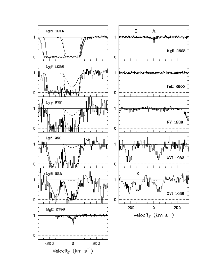
Figure 7: Model contributions to the subsystems, as in Figure 5, but with Model 2 used to represent subsystem A (see Table $2$). The dotted curves, representing the absorption contributions from the Mgii clouds in subsystem A, now make a negligible contribution to the Siiv absorption. The collisional component with $\log T=4.62$ is shown as a dashed curve. The long–dashed curves include contributions from both the Mgii clouds and the additional offset Siiv clouds (using a solar abundance pattern for both), as well as from the collisional component. The solid curve includes all of these contributions, but with a $0.5$ dex decrease in the abundances of carbon and silicon in the Mgii clouds of subsystem A. The subsystem B model is the same as for Figure 5, again with no abundance pattern adjustment. Additional transitions are shown in Figure 8.

Figure 8: As in Figure 7, synthesized spectra corresponding to model 2 are overplotted on the data for additional transitions. This model apperas to be a better fit than compared to model 1, shown in Figure 6. The dotted lines shown the contribution to the absorption from the Mgii clouds in subsystem A. The dashed line reveals the contribution from the collisionally ionized componenent that creates the smooth profile in the Siiii $\lambda 1207$ transition. The long-dashed line combines the four Mgii and four Siiv clouds as well as the collsionally ionized component with solar metallicity. The solid line shows our best fit to the data using model 2.

Figure 9: The left panel illustrates, for a metallicity of $\log Z=-1.0$, the effect of changing the ionization parameter of the two broad components that produce high ionization absorption. The dotted curves represent a model with an ionization parameter of $\log U=-1.5$, and the solid curves represent a model with $\log U=-0.5$. For both models, the abundance of nitrogen in the blue broad components has been reduced by $0.8$ dex. The subsystem contributions (important for Civ in subsystem A) are also included (using Model 2 for subsystem A). The middle panel is similar, but for $\log Z=-0.5$, and for $\log U=-1.5$ (dotted) and $\log U=-1.0$ (solid), with a $0.8$ dex reduction of nitrogen in the blue broad component. The right hand panel shows an acceptable model for the broad phases, with $\log Z=-0.5$ and $\log U=-1.5$ for the blue broad component and $\log Z=-1.0$ with $\log U=-0.5$ for the red broad component (see Table $3$). This model includes a reduction of the abundance of nitrogen by $\sim 0.8$ dex.

Table 1: Equivalent Widths

Transition	Subsystem A	Subsystem B	Total
Ly$\alpha$ $\lambda 1215$	$---$	$---$	$1.45\pm 0.01$
Ly$\beta$ $\lambda 1026$	$---$	$---$	$1.09\pm 0.03$
Ly$\gamma$ $\lambda 972$	$---$	$---$	$0.891\pm 0.04$
Ly$\delta$ $\lambda 950$	$---$	$---$	$0.859\pm 0.03$
Ly$8$ $\lambda 923$	$---$	$---$	$0.611\pm 0.04$
Mgii $\lambda 2796$	$0.097\pm 0.008$	$---$	$0.097\pm 0.008$
Mgii $\lambda 2803$	$0.046\pm 0.009$	$<0.006$	$<0.052$
Feii $\lambda 2600$	$<0.038$	$<0.038$	$<0.076$
Siii $\lambda 1260$	$0.024\pm 0.005$	$<0.008$	$<0.032$
Cii $\lambda 1335$	$0.067\pm 0.007$	$0.017\pm 0.004$	$0.084\pm 0.008$
Siiii $\lambda 1207$	$0.28\pm 0.007$	$0.14\pm 0.006$	$0.42\pm 0.009$
Siiv $\lambda 1394$	$0.20\pm 0.006$	$0.055\pm 0.004$	$0.255\pm 0.007$
Siiv $\lambda 1403$	$0.060\pm 0.006$	$0.024\pm 0.005$	$0.084\pm 0.008$
Nv $\lambda 1239$	$<0.010$	$<0.010$	$<0.020$
Ovi $\lambda 1032$	$0.094\pm 0.01$	$0.14\pm 0.01$	$0.23\pm 0.01$
Ovi $\lambda 1038$	$0.14\pm 0.01$	$0.092\pm 0.01$	$0.23\pm 0.01$
Civ $\lambda 1548$	$---$	$---$	$0.40\pm 0.02$
Civ $\lambda 1551$	$---$	$---$	$0.38\pm 0.02$

Note. — The equivalent widths were measured for various transitions detected at the $3$ sigma level. For transitions that were not detected, an $3$ sigma upper limit is given. Because both subsystems are blended together in the low resolution FOS data covering Civ, only a total equivalent width is shown. Although covered in the higher resolution STIS data, the two subsystems as traced by the Ly$\alpha$ are also blended and individual components can not be measured.

Table 2: Photoionized Cloud Properties

	$v$	$N_{\rm tot}$	$N({\hbox{{\rm H}\kern 1.00006pt{\sc i}}})$	$\log U$	$Z$	size	$N({\hbox{{\rm Mg}\kern 1.00006pt{\sc ii}}})$	$N({\hbox{{\rm Si}\kern 1.00006pt{\sc ii}}})$	$N({\hbox{{\rm C}\kern 1.00006pt{\sc ii}}})$	$N({\hbox{{\rm Si}\kern 1.00006pt{\sc iii}}})$	$N({\hbox{{\rm Si}\kern 1.00006pt{\sc iv}}})$	$N({\hbox{{\rm C}\kern 1.00006pt{\sc iv}}})$	$b$
	[km s-1]	[cm-2]	[cm-2]		[$Z_{\odot}$]	[kpc]	[cm-2]	[cm-2]	[cm-2]	[cm-2]	[cm-2]	[cm-2]	[km s-1]
Subsystem A - Model 1
Mgii1	$-35.4$	$19.5$	$16.4$	$-2.3$	$-1.4$	$8$	$11.45$	$11.5$	$12.6$	$12.6$	$12.3$	$13.4$	$5.82$
Mgii2	$-12.7$	$19.9$	$16.6$	$-2.5$	$-1.4$	$6$	$11.90$	$11.8$	$12.9$	$12.9$	$12.4$	$13.3$	$10.78$
Mgii3	$2.6$	$20.0$	$16.8$	$-2.3$	$-1.4$	$24$	$12.02$	$12.0$	$13.1$	$13.1$	$12.7$	$13.8$	$3.07$
Mgii4	$18.3$	$19.7$	$16.5$	$-2.3$	$-1.4$	$13$	$11.68$	$11.7$	$12.8$	$12.8$	$12.5$	$13.6$	$5.92$
Subsystem A - Model 2
Mgii1	$-35.4$	$18.3$	$16.1$	$-3.1$	$-1.4$	$0.09$	$11.45$	$11.1$	$12.2$	$11.9$	$10.9$	$11.4$	$5.82$
Mgii2	$-12.7$	$18.8$	$16.5$	$-3.1$	$-1.4$	$0.2$	$11.90$	$11.5$	$12.6$	$12.3$	$11.4$	$11.8$	$10.78$
Mgii3	$2.6$	$18.9$	$16.6$	$-3.1$	$-1.4$	$0.3$	$12.02$	$11.6$	$12.8$	$12.4$	$11.5$	$11.9$	$3.07$
Mgii4	$18.3$	$18.6$	$16.3$	$-3.1$	$-1.4$	$0.1$	$11.68$	$11.3$	$12.9$	$12.1$	$11.2$	$12.1$	$5.92$
Siiv1	$-30.3$	$19.0$	$15.8$	$-2.3$	$-1.4$	$2$	$10.9$	$11.4$	$12.1$	$12.5$	$12.2$	$12.9$	$5.7$
Siiv2	$-7.8$	$18.9$	$15.8$	$-2.3$	$-1.4$	$2$	$10.8$	$11.4$	$12.0$	$12.5$	$12.2$	$12.8$	$11.0$
Siiv3	$3.9$	$19.3$	$16.1$	$-2.3$	$-1.4$	$5$	$11.2$	$11.7$	$12.4$	$12.8$	$12.5$	$13.2$	$5.0$
Siiv4	$23.3$	$19.1$	$16.0$	$-2.3$	$-1.4$	$3$	$11.1$	$11.6$	$12.3$	$12.7$	$12.4$	$13.1$	$3.0$
Subsystem B
Siiii1	$-184.5$	$17.9$	$15.3$	$-2.7$	$-1.4$	$0.08$	$10.5$	$10.8$	$11.9$	$11.8$	$11.2$	$12.0$	$12.75$
Siiii2	$-144.9$	$18.9$	$16.2$	$-2.7$	$-1.4$	$0.8$	$11.5$	$11.8$	$12.9$	$12.8$	$12.2$	$13.0$	$22.00$
Siiii3	$-127.7$	$18.5$	$15.8$	$-2.7$	$-1.4$	$0.3$	$11.1$	$11.4$	$12.5$	$12.4$	$11.8$	$12.6$	$6.48$

Note. — Cloud properties are summarized for example of Model 1 (just 4 Mgii clouds) and Model 2 (4 Mgii clouds and 4 offset Siiv clouds) for subsystem A. Subsystem B properties are also given. For both models, the abundances of silicon and carbon for the Mgii clouds of subsystem A are adjusted downwards from solar by $0.5$ dex. All column densities are indicated as logs of the values in units of cm^-2. Column densities of the Mgii and Siiv clouds from subsystem A as well as the Siiii clouds from subsystem B were determined by Voigt-profile fits. Also included is the total Hydrogen column density, $N_{(}tot)$, (including Hi and Hii). The velocities, also determined by VP fits, are measured relative to the median of the apparent optical depth distribution for the Mgii clouds. Doppler parameters listed in the last column correspond to the transition for which that cloud is optimized (listed in the first column). The models summarized in this table are also shown in Figures 5, 6, 7 and 8.

Table 3: Photoionized Cloud Properties

	$v$	$N_{\rm tot}$	$N({\hbox{{\rm H}\kern 1.00006pt{\sc i}}})$	$\log U$	$Z$	size	$N({\hbox{{\rm C}\kern 1.00006pt{\sc iv}}})$	$N({\hbox{{\rm N}\kern 1.00006pt{\sc v}}})$	$N({\hbox{{\rm O}\kern 1.00006pt{\sc vi}}})$	$b$
	[km s-1]	[cm-2]	[cm-2]		[$Z_{\odot}$]	[kpc]	[cm-2]	[cm-2]	[cm-2]	[km s-1]
Broad Components
Hi	$-210.2$	$18.9$	$15.0$	$-1.5$	$-0.5$	$12$	$14.3$	$13.0$	$14.4$	$27$
Hi	$40.3$	$19.2$	$14.0$	$-0.5$	$-1.0$	$257$	$12.5$	$12.8$	$14.2$	$37$

Note. — All column densities are indicated as logs of the values in units of cm^-2. Column densities of the two broad components were determined by Voigt-profile fits to Ly$\alpha$. Doppler parameters listed in the last column correspond to the transition for which that cloud is optimized (listed in the first column). The values shown in this table represent a plausible model for the broad components, using Model 2 for subsystem A, also shown in Figure 9. The blue broad component has an abundance pattern in which nitrogen is $0.8$ dex deficient relative to other elements. The choice of model for subsystem A only slightly affects the parameters for the blue broad component.

References

- Bahcall et al. (1993) Bahcall, J. N., et al. 1993, ApJS, 87, 1
- Bahcall et al. (1996) Bahcall, J. N., et al. 1996, ApJ, 457, 19
- Bergeron & Boissé (1991) Bergeron, J., & Boissé, P. 1991, A&A, 243, 344
- Bergeron et al. (1992) Bergeron, J., Cristiani, S., & Shaver, P. A. 1992, A&A, 257, 417
- Bond et al. (2001) Bond, N. A., Churchill, C. W., Charlton C. C., & Vogt, S. S., 2001, ApJ, 562, 641
- Bowen, Tripp, & Jenkins (2001) Bowen, D. V., Tripp, T. M., & Jenkins, E. B. 2001, AJ, 121, 1456
- Brown et al. (2002) Brown, T. et al. 2002, HST STIS Data Handbook, version 4.0, ed.. Mobasher, Baltimore, STScI
- Bruzual & Charlot (1993) Bruzual, A. G., & Charlot, S. 1993, ApJ, 405, 538
- Charlton & Churchill (1998) Charlton, J. C., & Churchill, C. W. 1998, ApJ, 499, 181
- Charlton et al. (2000) Charlton, J. C., Mellon, R. R., Rigby, J. R., & Churchill, C. W. 2000 ApJ, 545, 645
- Charlton et al. (2003) Charlton, J. C., Ding, J., Zonak, S. G., Churchill, C. W., Bond, N. A., & Rigby, J. R. 2003, ApJ, 589, 311
- Chen, Hou, & Wang (2003) Chen, L., Hou, J. L., & Wang, J. J. 2003, AJ, 125, 1397
- Churchill et al. (2000) Churchill, C. W., Mellon, R. R., Charlton, J. C., Jannuzi, B. T., Kirhakos, S., Steidel, C. C., & Schneider, D. 2000, ApJS, 130, 91
- Churchill et al. (1999) Churchill, C. W., Rigby, J. R., Charlton, J. C., & Vogt, S. S. 1999, ApJS, 120, 51
- Churchill & Vogt (2001) Churchill, C. W., & Vogt, S. S. 2001, AJ, 122, 679
- Dahlem, Weaver, & Heckman (1998) Dahlem, M., Weaver, K. A., & Heckman, T. M. 1998, ApJS, 118, 401
- D’Odorico & Petitjean (2001) D’Odorico, V., & Petitjean, P. 2001, A&A, 370, 729
- Ding et al. (2003a) Ding, J., Charlton, J. C., Zonak, S. G., & Churchill, C. W. 2003a, ApJ, 587, 551
- Ding et al. (2003b) Ding, J., Charlton, J. C., Churchill, C. W., & Palma, C. 2003b, ApJ, 590, 746
- Farrah et al. (2002) Farrah, D., Verma, A., Oliver, S., Rowan–Robinson, M. & McMahon, R. 2002, MNRAS, 329, 605
- Ferland (2001) Ferland, G. 2001, Hazy, A Brief Introduction to Cloudy 96.00
- Haardt & Madau (1996) Haardt, F., & Madau, P. 1996, ApJ, 461, 20
- Heckman et al. (2000) Heckman, T. M., Lehnert, M. D., Strickland, D. K., & Armus, L. 2000, ApJS, 129, 493
- Henry, Edmunds, & Köppen (2000) Henry, R. B. C., Edmunds, M. G., & Köppen, J. 2000, ApJ, 541, 660
- Howk et al. (2002) Howk, J. C., Sembach, K. R., Savage, B. D., Massa, D., Friedman, S. D., & Fullerton, A. W. 2002, ApJ, 569, 214
- Hurwitz, Jelinsky, & Dixon (1997) Hurwitz, M., Jelinsky, P., Dixon, W. V. D. 1997, ApJ, 481 L31
- Jannuzi et al. (1998) Jannuzi, B. T., et al. 1998, ApJS, 118, 1
- Kimble et al. (1998) Kimble, R. A., et al. 1998, ApJ, 492, L83
- Le Brun et al. (1993) Le Brun, V., Bergeron, J., Boissé, P., & Christian, C. 1993, A&A, 279, 33
- Martin (2003) Martin, C. L. 2003, in “The IGM/Galaxy Connection: The Distribution of Baryons at ”, eds. J. L. Rosenburg and M. E. Putman (Kluwer:Dordrecht), p. 205
- Martin, Kobulnicky, & Heckman (2002) Martin, C. L., Kobulnicky, H. A., Heckman, T. M., 2002, ApJ, 574, 663
- Mateo (1998) Mateo, M. 1998, ARAA, 36, 435
- Pettini (2003) Pettini, M. 2003, in “Cosmochemistry: The Melting Pot of Elements”, (Cambridge University Press: Cambridge), in press
- Ptak et al. (1997) Ptak, A., Serlemitsos, P., Yaqoob, T., Mushotzky, R.,& Tsuru, T. 1997, AJ, 113, 1286
- Rao & Turnshek (2000) Rao, S. M., & Turnshek, D. A. 2000, ApJS, 130, 1
- Read, Ponman, & Strikland (1997) Read, A. M., Ponman, T. J., & Strickland, D. K. 1997, MNRAS, 286, 626
- Rigby et al. (2002) Rigby, J. R., Charlton, J. C. & Churchill, C. W., 2002, ApJ, 565, 743
- Rosenberg et al. (2003) Rosenberg, J. L., Ganguly, R., Giroux, M. L., & Stocke, J. T. 2003, ApJ, in press
- Savage et al. (2002) Savage, B. D., Sembach, K. R., Tripp, T. M., & Richter, P. 2002, ApJ, 564, 631
- Savage et al. (2003) Savage, B. D., Sembach, K. R., Wakker, B. P., Richter, P., Meade, M., Jenkins, E. B., Shull, J. M., Moos, H. W., & Sonneborn, G. 2003, ApJS 146, 125
- Schneider et al. (1993) Schneider et al. 1993, ApJS, 87, 45
- Steidel (1995) Steidel, C.C. 1995, in QSO Absorption Lines, ed. G. Meylan (Garching : Springer Verlag), 139
- Steidel et al. (1997) Steidel. C. C., Dickinson, M., Meyer, D. M., Adelberger, K. L., & Sembach, K. R. 1997, ApJ, 480, 568
- Steidel, Dickinson, & Persson (1994) Steidel, C. C., Dickinson, M. & Persson, E. 1994, ApJ, 437, L75
- Steidel et al. (2002) Steidel, C. C., Kollmeier, J. A., Shapley, A. E., Churchill, C. W., Dickinson, M., & Pettini, M. 2002, ApJ, 570, 526
- Steidel & Sargent (1992) Steidel, C. C., & Sargent, W. L. W. 1992, ApJS, 80, 1
- Sutherland & Dopita (1993) Sutherland, R.S., & Dopita, M.A., 1993, ApJS, 88, 253
- Theuns, Mo, & Schaye (2001) Theuns, T., Mo, H. J., & Schaye, J. 2001, MNRAS, 321, 450
- Tripp et al. (2002) Tripp, T. M., et al. 2002, ApJ, 575, 697