A DENSE-CLOUD MODEL FOR GAMMA-RAY BURSTS
TO EXPLAIN BIMODALITY

Abstract

In this model a collimated ultra-relativistic ejecta collides with an amorphous dense cloud surrounding the central engine, producing gamma-rays via synchrotron process. The ejecta is taken as a standard candle, while assuming a gaussian distribution in thickness and density of the surrounding cloud. Due to the cloud high density, the synchrotron emission would be an instantaneous phenomenon (fast cooling synchrotron radiation), so a GRB duration corresponds to the time that the ejecta takes to pass through the cloud. Fitting the model with the observed bimodal distribution of GRBs’ durations, the ejecta’s initial Lorentz factor, and its initial opening angle are obtained as $\Gamma_{0}\lesssim 10^{3}$, and $\zeta_{0}\approx 10^{-2}$, and the mean density and mean thickness of the surrounding cloud as $\overline{n}\sim 3\times 10^{17}cm^{-3}$ and $\overline{L}\sim 2\times 10^{13}cm$. The clouds maybe interpreted as the extremely amorphous envelops of Thorne-Zytkow objects. In this model the two classes of long and short duration GRBs are explained in a unique frame.

1 INTRODUCTION

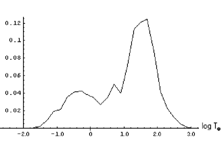
Figure 1: Distribution of log of GRBs’ time Duration (normalized), obtained from data of BATSE 4th catalog.

Undoubtedly, gamma-ray bursts (GRBs) have remained to be one of the most exiting, intriguing, and enigmatic astrophysical phenomena since their mysterious discovery in the past several decades (for a recent expository review of GRBs the interested reader is referred to the excellent work by J. I. Katz katz (2002)). Although no two GRBs resemble each other and each one has its own peculiarities which makes the problem of modeling GRBs very difficult, the whole of GRBs reveals several interesting features. Since the publication of the BATSE data (Fishman et al., 1993) which included the observation of over $200$ GRBs and revealed an almost uniform distribution of the location of GRBs in the sky, combined with the deficiency of faint GRBs, the association of GRBs with the galactic plane has been ruled out. The successive publications confirmed the figure more and more (Meegan et al., 1996; Paciesas et al., 1999). However, since the observation of afterglows in X-ray (Costa et al., 1997), optical (van Paradijs et al., 1997) and radio spectrum (Frail et al., 1997) and the advert of Robotic Optical Transient Search Experiment (ROTSIE) telescope (Akerlof et al., 2003; Gisler et al., 1999, e.g.) which has revealed the red shifts for several GRBs, their cosmological origin is widely accepted.
The BATSE data (Fishman et al., 1993; Meegan et al., 1996; Paciesas et al., 1999) has also revealed another equally important overall feature of the GRBs. The distribution of time duration in observed GRBs shows a double heap distribution, which the smaller one peaks around 0.2 sec and the larger one peaks around 20 sec (Fig.1). This two peaked distribution which apparently separated GRBs into the so called short duration and long duration ones was referred to as bimodality (Kouveliotou et al., 1993; Norris et al., 1993) and led some investigators to believe that there are two distinct populations of GRBs.
It has been widely believed that whatever the central engine is, the radiation reaching us originates from the space surrounding the central engine. It is also believed that during the collapse the energy release streams out in relativistic confined ejectas (not isotropically) and thus the total energy release during each event is far less than the unbelievable amount that one might obtain by assuming isotropic radiation (Kulkarni et al., 1999).
The aim of this paper is to present a rather simple model, based on these general ideas, and show that there is no need for assuming two distinct populations of GRBs, and to show that once the geometrical considerations and cosmological effects are fully accounted for a genetic standard candle ejecta, crossing an amorphous dense cloud, the so called bimodality can be deduced.
In § 2 the model and its general formulation is introduced. In § 3 the computational results and the fit of model parameters with BATSE data will be presented as well. § 4 is devoted to a discussion on the results. Some needed calculations and discussions are presented in appendices.

2 THE MODEL FORMULATION

GRBs are modeled as a central engine with an instantaneous ultra-relativistic jet of material surrounded by an amorphous dense cloud. The central engine and its jet are taken as a standard candle with a total release energy of $E$, and an initial Lorentz factor $\Gamma_{0}$ and initial opening angle $\zeta_{0}$ of the jet for all GRBs, whereas the clouds are considered to have a distribution both in thickness as well as in density. For the sake of illustration and brevity we take both of these distributions to be Gaussian.
We want to calculate the distribution of logarithm of time duration of observed GRBs according to the above model. We should however explore the ejecta evolution since the observed gamma ray emission originates in the shock front of ejecta+shocked medium.

2.1 The Ejecta Evoution

The equations describing the ejecta evolution are presented here, based on the notations of Paczynski & Rhoads Paczynski and Rhoads (1993). We consider the cloud to be at a distance $r_{0}$ from the source, which may be negligible in comparison to the cloud thickness $L$. The ratio of swept-up mass to ejecta mass $M_{0}$ has the form below:

$$f=\frac{1}{M_{0}}\int^{r}_{r_{0}}\rho\Omega_{m}(r^{\prime})r^{\prime 2}dr^{\prime},$$ (1)

where, $r$ is the ejecta distance from the source. The cloud density $\rho$ is taken to be independent of $r$. Furthermore, $\Omega_{m}(r)=2\pi[1-\cos\zeta(r)]$, in which $\zeta(r)$ represents the opening angle of the ejecta at radius $r$. So, equation(1) can be written as:

$$\frac{df}{dr}=2\pi n\frac{m_{p}\Gamma_{0}c^{2}}{E}[1-\cos\zeta(r)]r^{2},$$ (2)

where $E$ and $\Gamma_{0}$ are the initial kinetic Energy and initial Lorentz factor of the ejecta ($E=\Gamma_{0}M_{0}c^{2}$), and $n$ denotes the number density of the cloud ($\rho=m_{p}\>n$). Paczynski & Rhoads Paczynski and Rhoads (1993) derived the relation between $f$ and $\Gamma$ from conservation of energy and momentum. Here, we use their relation in a form suitable for our computations:

$$\frac{df}{d\Gamma}=-\frac{\sqrt{\Gamma_{0}^{2}-1}}{\sqrt[3]{\Gamma^{2}-1}}~{}.$$ (3)

The ejecta’s opening angle $\zeta(r)$ increases with increasing $r$ as a result of lateral spreading of the cloud of ejecta+swept-up matter in the comoving frame at the sound speed $c_{s}$, which has been derived by Rhoads Rhoads (1998) to be as below:

$$d\zeta(r)=\frac{c_{s}\>dt_{co}}{r},$$ (4)

where $t_{co}$ denotes the time from the event, measured in the ejecta comoving frame. Substituting $dt_{co}=dt/\Gamma$, and $dt=dr/\beta c$, we have :

$$\frac{d\zeta(r)}{dr}=\frac{c_{s}/c}{\beta\>\Gamma\>r}.$$ (5)

Now, eliminating $f$ between equations(2) and (3) yields:

$$\frac{d\Gamma}{dr}=-2\pi n\frac{m_{p}\Gamma_{0}c^{2}}{E}[1-\cos\zeta(r)]\frac{\sqrt[3]{\Gamma^{2}-1}}{\sqrt{\Gamma_{0}^{2}-1}}r^{2}~{}.$$ (6)

Let’s rewrite equations(5) and (6) in a non-dimensional form as below:

$$\left\{\begin{array}[]{rcl}\frac{d\zeta}{d\eta}&=&\frac{c_{s}/c}{\eta\Gamma(\eta)(1-\frac{1}{\Gamma^{2}})^{-1/2}}\\ \frac{d\Gamma}{d\eta}&=&-\frac{\Gamma_{0}\sqrt[3]{\Gamma^{2}-1}}{\sqrt{\Gamma_{0}^{2}-1}}[1-\cos\zeta(\eta)]\eta^{2}\end{array}\right.\\ ,$$

where, the non-dimensional parameter $\eta$ is defined as:

$$\eta\equiv\frac{r}{l(n/E)},$$ (7)

in which:

$$l(n/E)\equiv\left(\frac{2\pi m_{p}c^{2}n}{E}\right)^{-1/3}=4.75\times 10^{11}\left(\frac{n_{18}}{E_{48}}\right)^{-1/3}\>\>cm~{}.$$ (8)

These coupled first order differential equations can be solved numerically by introducing the initial conditions:

$$\left\{\begin{array}[]{rcl}\Gamma(\eta_{0})=\Gamma_{0}\\ \zeta(\eta_{0})=\zeta_{0}\end{array}\right.\\ ,$$

where $\eta_{0}\equiv r_{0}/l(n/E)$.
Noting that $\beta=dr/cdt=(1-1/\Gamma^{2})^{1/2}$, we have:

$$\frac{d\tau}{d\eta}=\left(1-\frac{1}{\Gamma^{2}(\eta)}\right)^{-1/2}~{}~{}~{};~{}~{}~{}\tau(\eta_{0})=0.$$ (9)

In equation(11) we used equation(8) and a non-dimensional time parameter $\tau$ defined as:

$$\tau\equiv\frac{c\>t}{l(n/E)}$$ (10)

The numerical results of equation(11) are used in appendix C, where we consider the effect of burster geometry on the observable time duration.

2.2 Formulation of Time Duration Distribution

We begin with introducing the probability density for a collimated burst to occur in a direction through the cloud with a thickness $L$ and a number density $n$. We assume the cloud thickness to have a gaussian distribution in various directions from the central engine. By assuming a gaussian distribution for the cloud density as well we have:

$$\frac{d^{3}p}{dn\>dL\>d\Omega}=\frac{1}{4\pi}\frac{1}{\sqrt{2\pi}\sigma_{{}_{n}}}\>\exp\left[\frac{-(n-\overline{n})^{2}}{2\sigma_{{}_{n}}^{2}}\right]\>\frac{1}{\sqrt{2\pi}\sigma_{{}_{L}}}\>\exp\left[\frac{-(L-\overline{L})^{2}}{2\sigma_{{}_{L}}^{2}}\right]~{}.$$ (11)

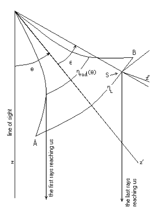
Figure 2: Geometry of Radiation. In the figure, $\eta_{rad}(\theta)$ denotes the radius where the radiation angle $\zeta_{rad}$ becomes equal to $\theta$ (see appendix C). As shown in the figure (for $\theta$’s larger than $\zeta_{rad}(\eta_{0})$) the first photons reaching us are those emitted from the edge of the shock front at this radius. If $\epsilon(\eta_{{}_{L}},\theta)<\zeta(\eta_{{}_{L}})$, then the last photons reaching us are those emitted from $\epsilon=\epsilon(\eta_{{}_{L}},\theta)$ on the shock front (point S in the figure). The point S would be the furthest visible point on the shock front, since the line of sight fells out of the radiation cone of the points farther than it (points between S and B). If $\epsilon(\eta_{{}_{L}},\theta)>\zeta(\eta_{{}_{L}})$, then the point B would be the last visible point (see Eqn.[C15]).

The quantities $\overline{L}$ and $\sigma_{{}_{L}}$ denote the mean thickness of the cloud and its dispersion, respectively. Likewise, $\overline{n}$ and $\sigma_{{}_{n}}$ are defined in a similar manner. Denoting the angle between the ejecta symmetry axis and the line of sight by $\theta$ (Fig.2), and considering the independence of the probability density from azimuth angle in equation(13), we can write:

$$\frac{d^{3}p}{dn\>dL\>d\theta}=\frac{2\pi\>\sin\theta}{4\pi}\frac{1}{\sqrt{2\pi}\sigma_{{}_{n}}}\>\exp\left[\frac{-(n-\overline{n})^{2}}{2\sigma_{{}_{n}}^{2}}\right]\>\frac{1}{\sqrt{2\pi}\sigma_{{}_{L}}}\>\exp\left[\frac{-(L-\overline{L})^{2}}{2\sigma_{{}_{L}}^{2}}\right]~{}.$$ (12)

The synchrotron emission is a fast process for our model (see appendix A), so $T_{rec}$ (the time duration of a GRB as measured by an observer cosmologicaly near to the source and located on the line of sight), is attributed to the time that the shock front takes to cross the dense cloud. As explained in appendix C, the cloud thickness $L$ can be expressed as a function of $\theta$, $n$, and $T_{rec}$ (Eqn.[C16]):

$$L=L(T_{rec},n,\theta)~{}.$$ (13)

So we write:

$$\frac{d^{2}}{dn\>d\theta}\>\left(\frac{dp}{dL}\right)=\frac{d^{2}}{dn\>d\theta}\left(\frac{dp}{dT_{rec}}\right)_{{}_{n,\theta}}\>\left(\frac{dT_{rec}}{dL}\right)_{{}_{n,\theta}}~{},$$ (14)

or:

$$\frac{d^{3}p}{dn\>d\theta\>d\log T_{rec}}=\frac{d^{3}p}{dn\>d\theta\>dL}\left(\frac{dL}{d\log T_{rec}}\right)_{{}_{n,\theta}}~{},$$ (15)

notifying that by this substitution(Eqn.[15]), the bursts that do not manage to cross through the cloud with a thickness $L$ (and stop in it) are practically omitted (see appendix C). Using equation(14) in equation(17), it is seen that:

$$\frac{d^{3}p}{dn\>d\theta\>d\log T_{rec}} = \frac{\sin\theta}{4\pi}\frac{1}{\sigma_{{}_{n}}\>\sigma_{{}_{L}}}\left(\frac{dL}{d\log T_{rec}}\right)_{{}_{n,\theta}}$$ (16)

$$\times \>\exp\left[\frac{-(n-\overline{n})^{2}}{2\sigma_{{}_{n}}^{2}}\right]\exp\left[\frac{-(L(T_{rec},n,\theta)-\overline{L})^{2}}{2\sigma_{{}_{L}}^{2}}\right].$$

Integrating over $\theta$ and $n$ yields:

$$\frac{dp}{d\log T_{rec}}=\frac{1}{4\pi\sigma_{{}_{n}}\sigma_{{}_{L}}}\int_{\theta=0}^{\frac{\pi}{2}}\int_{n=0}^{\infty} \exp\left[\frac{-(n-\overline{n})^{2}}{2\sigma_{{}_{n}}^{2}}\right]\exp\left[\frac{-(L(T_{rec},n,\theta)-\overline{L})^{2}}{2\sigma_{{}_{L}}^{2}}\right]$$ (17)

$$\times \left(\frac{dL}{d\log T_{rec}}\right)_{{}_{n,\theta}}\sin\theta\>d\theta\>dn~{}.$$

The effect of red shift is not considered yet. Equation(19) only gives the probability density for an observed burst to have a specified logarithm of time duration, as measured by an observer near to it. We now investigate the relation between $dp/d\log T_{rec}$ and $dp/d\log T_{\oplus}$ where $T_{\oplus}$ stands for the time duration of a GRB measured at Earth. To obtain the later, the former must be integrated over red shift z, using a weight function $F_{{}_{GRB}}(z)$, so that $F_{{}_{GRB}}(z)\>dz$ represents the probability for occurring a GRB in a red shift between $z$ and $z+dz$. To show this, let’s consider an observer located on the line from us to an occurred GRB which is (cosmologicaly) near to it. The probability density for the GRB to occur in a red shift z (with respect to us), and to have a specific $\log T_{rec}$ (measured by the observer near to the GRB), is clearly as below:

$$\frac{d^{2}p}{dz\>d\log T_{rec}}=F_{{}_{GRB}}(z)\frac{dp}{d\log T_{rec}}~{}.$$ (18)

To obtain $d^{2}p/dz\>d\log T_{\oplus}$, which is the probability density for observing a GRB occurred at a red shift z and observed to have a specific $T_{\oplus}$, we write:

$$\frac{d^{2}p}{dz\>d\log T_{\oplus}}=\frac{d}{dz}\left(\frac{dp}{d\log T_{\oplus}}\right)_{z}=\frac{d}{dz}\left[\left(\frac{dp}{d\log T_{rec}}\right)_{z}\left(\frac{d\log T_{rec}}{d\log T_{\oplus}}\right)_{z}\right]~{},$$ (19)

noting that $T_{\oplus}=(1+z)T_{rec}$, the second term in the the bracket equals one. Now, using equation(20) we have :

$$\frac{d^{2}p}{dz\>d\log T_{\oplus}}=F_{{}_{GRB}}(z)\>\left(\left.\frac{dp}{d\log T_{rec}}\right|_{T_{rec}=T_{\oplus}/(1+z)}\right)~{},$$ (20)

After integrating equation(22) over z, the final form of the observable probability density will be as below:

$$\frac{dp}{d\log T_{\oplus}}=\int_{z=0}^{\infty}F_{{}_{GRB}}(z)\>\left(\left.\frac{dp}{d\log T_{rec}}\right|_{T_{rec}=T_{\oplus}/(1+z)}\right)\>dz\>~{}.$$ (21)

The explicit form of $F_{{}_{GRB}}(z)$ is needed. This form is obtained in appendix D (Eqn.[D4] and Eqn.[D5]). The second term in the integrand is given by equation(19), in which the implicit form of $L(T_{rec},n,\theta)$ appears. Appendix C is devoted to the procedure of obtaining this function. For evaluation of $dp/d\log T_{\oplus}$ (Eqn.[23]), we need the values of eight parameters. Four of them are the cloud parameters $\overline{L}$, $\sigma_{L}$, $\overline{n}$, and $\sigma_{n}$, and the fifth one is the index $q$ corresponding to the GRB occurrence rate (see Eqn.[D5]). The later three ones are the ejecta parameters, $E$, $\Gamma_{0}$, and $\zeta_{0}$, which are the initial kinetic energy, the initial Lorentz factor, and the initial opening angle of the ejecta, respectively.

3 NUMERICAL COMPUTATIONS AND RESULTS

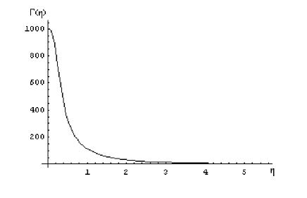
Figure 3: The Lorentz factor of shocked medium $\Gamma(\eta)$ versus the non-dimensional radius $\eta$, with $\Gamma_{0}=1000$ and $\zeta_{0}=0.01$ (see Eqn.[7]).

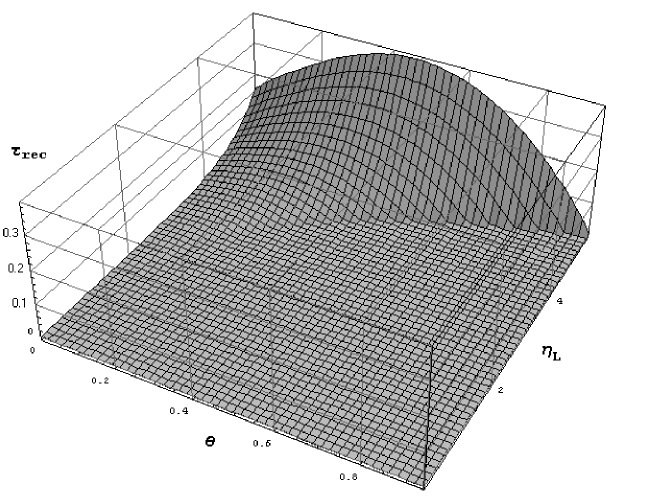
Figure 4: The evaluated non-dimensional time duration $\tau_{rec}(\theta,\eta_{{}_{L}})$ of GRBs, versus $\theta$ and $\eta_{{}_{L}}$, with $\Gamma_{0}=1000$ and $\zeta_{0}=0.01$, (see appendix C).

The Mathmatica 4 software is used in the numerical computations. In the procedure we begin with solving the coupled differential equations(7) and (11) which govern the ejecta evolution, and in which $\Gamma_{0}$ and $\zeta_{0}$ are the only free parameters. Furthermore, we take $\eta_{0}=0$. For fixed values of these parameters, the functions $\Gamma(\eta)$, $\tau(\eta)$ and $\zeta_{rad}(\eta)$ (see Eqn.[C3]) can be uniquely obtained . Obviously $\Gamma$ decreases with increasing $\eta$ (Fig.3), and reaches to $\Gamma=1$ when $\eta$ approaches a certain value. This in fact takes an infinite time and results in an infinite non-dimensional time duration $\tau_{rec}$ (see Eqn.[C4] and Eqn.[C5]). So, to circumvent the difficulty, we consider an effective lower limit $\Gamma_{min}$ for the Lorentz factor of shocked matter, which yields an effective upper limit for non-dimensional time $\tau$. We adopted $\Gamma_{min}=2$ as a lower cut-off. Then, following the procedure explained in appendix C, for a specific cloud thickness $L$, and correspondingly a specific $\eta_{{}_{L}}$ (Eqn.[C13]), the non-dimensional time duration $\tau_{rec}(\theta,\eta_{{}_{L}})$ of a GRB can be calculated for every $\theta$ and $\eta_{{}_{L}}$ (Fig.4). Let’s denote the radius corresponding to $\Gamma_{min}$ by $\eta_{m}$ so that $\Gamma_{min}\equiv\Gamma(\eta_{m})$, and recall that in the model, for $\eta_{m}<\eta_{{}_{L}}$, the emitted photons would be completely scattered by the electrons of not-swept part of the cloud (that they have to pass through, before entering free space; see appendix C), and so, the whole phenomenon may be called a ”failed GRB ”. But, if $\eta_{m}>\eta_{{}_{L}}$, the shocked matter succeeds to go out of the cloud and, as explained in § 4.3, due to a suppression process that intensively decreases the cross-section of Compton scattering,(the major part of)the emitted photons finally succeed to get released from the shocked medium and enter free space, provided that $\zeta(\eta_{{}_{L}})>[\sqrt{5/3}\>\Gamma(\eta_{{}_{L}})]^{-1}$ (see appendix B). It is really for this reason that $\tau_{rec}$ happens to be a function of $\eta_{{}_{L}}$, and practically independent of $\eta_{m}$. Then, solving $\tau_{rec}(\theta,\eta_{{}_{L}})$ for $\eta_{{}_{L}}$ numerically, we can obtain the function $\eta_{{}_{L}}(\tau_{rec},\theta)$ which is the equivalent non-dimensional form of expression (15). We rewrite equation(19) in a non-dimensional form suitable for numerical computations:

$$\frac{dp}{d\log\tau_{rec}}=\frac{1}{2\varrho\>\varsigma}\int_{\theta=0}^{\frac{\pi}{2}}\int_{\nu=0}^{\infty} \exp\left[\frac{-(\nu-1)^{2}}{2\varrho^{2}}\right]\exp\left[\frac{-\left(\frac{l(\overline{n}\nu/E)}{\overline{L}}\eta_{{}_{L}}(\tau_{rec},\theta)-1\right)^{2}}{2\varsigma^{2}}\right]$$ (22)

$$\times \frac{l(\overline{n}\nu/E)}{\overline{L}}\left(\frac{d\eta_{{}_{L}}}{d\log\tau_{rec}}\right)_{{}_{\nu,\theta}}\sin\theta\>d\theta\>d\nu,$$

in which, equation(C13) and the definitions below:
$\nu\equiv n/\overline{n}$ ,
$\varrho\equiv\sigma_{n}/\overline{n}$ ,
and
$\varsigma\equiv\sigma_{L}/\overline{L}$
are used. So, after choosing the quantities $\overline{L}$, $\sigma_{{}_{L}}$, $\overline{n}$, $\sigma_{n}$, and of course $E$, we can evaluate the integral appearing in equation(24). Then, after choosing a value for $q$, the integral of equation(23) can be performed to obtain the observable quantity $dp/d\textit{log}T_{\oplus}$.
As seen in equation(24), the initial kinetic energy $E$ and the cloud mean density $\overline{n}$ appear only in the form $E/\overline{n}$, and therefore they can not be found separately in a fitting process, and all that can be obtained is only their ratio. But, the observed fluence of GRBs reveals that the released energy in GRBs is of order of $E_{iso}\sim 10^{52}ergs$ for a isotropic burst, which reduces to $(\Omega/4\pi)E_{iso}$ if the bursts were confined to a cone with a solid angle $\Omega$. We used this amount of isotropic energy to relate $E$ to $\zeta_{0}$ ($E\equiv E_{iso}\zeta_{0}^{2}/2$), and reduce the free parameters of the model to seven as $\Gamma_{0},\zeta_{0},\overline{L},\sigma_{{}_{L}},\overline{n}$, $\sigma_{n}$ and $q$, which hereafter are called $\Pi$ parameters. These parameters must be chosen so that the results make the best fitting to the observed distribution of GRBs. To achieve the task, one must search in the seven dimensional $\Pi$ space, and find the point in which the statistical quantity $\chi^{2}$ takes the smallest value $\chi^{2}_{min}$. We used the BATSE 4th catalogue (Paciesas et al., 1999) of 1234 GRBs and adopted the bins $\Delta\log T_{\oplus}=0.2$ in a range $-1.9\leq\log T_{\oplus}<2.9$, and used the gradient search technique to move toward the best point in which $\chi^{2}$ gets minimized. The obtained fitted values are:

$$\Gamma_{0} = 0.97\times 10^{3}\>\>\>\>\>\>\>\>\>\>\>\zeta_{0}=0.01$$

$$\overline{L} = 1.7\times 10^{13}cm\>\>\>\>\>\>\>\>\overline{n}=2.9\times 10^{17}cm^{-3}$$

$$\sigma_{{}_{L}} = 0.21\overline{L}\>\>\>\>\>\>\>\>\>\>\>\>\>\>\>\>\>\>\>\>\sigma_{n}=0.71\overline{n}$$

$$q = -0.70$$ (23)

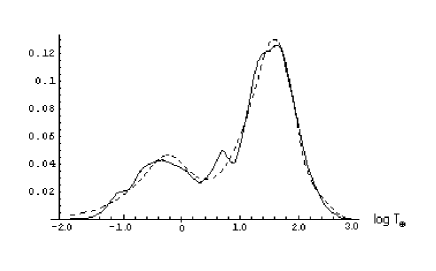
Figure 5: Results of best fitting. The solid curve shows the observed time duration distribution and the dashed one is calculated using the best of values for the model parameters. $\chi^{2}_{min}=1.4pdf$ (see § 3).

with a corresponding value $\chi^{2}_{min}=1.4$ (per degree of freedom). As can be seen in Fig.5, the deviation from a more perfect coincidence to data seems for the structure in the observed distribution located around $\log T_{\oplus}\sim 0.7$. The structure has been noted before (Yu et al., 1998). We put aside the the data of the noted structure, which are ones with durations between $0.3<\log(T_{\oplus})<0.9$, and again repeated the numerical searching process in the parametric space. The new obtained values of the fitted parameters are:

$$\Gamma_{0} = 0.96\times 10^{3}\>\>\>\>\>\>\>\>\>\>\>\zeta_{0}=0.01$$

$$\overline{L} = 1.8\times 10^{13}cm\>\>\>\>\>\>\>\>\overline{n}=2.9\times 10^{17}cm^{-3}$$

$$\sigma_{{}_{L}} = 0.21\overline{L}\>\>\>\>\>\>\>\>\>\>\>\>\>\>\>\>\>\>\>\>\sigma_{n}=0.71\overline{n}$$

$$q = -0.70$$ (24)

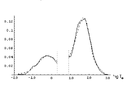
Figure 6: Results of best fitting. Same as Fig.5 with the data corresponding to the structure with $0.3<\log T_{\oplus}<0.9$ were cut. $\chi^{2}=1.1pdf$ (see § 3).

which slightly differ from what previously obtained (Eqn.[25]). But this time, $\chi^{2}_{min}$ reduces to $1.1$ (Fig.6). So the mentioned structure may be interpreted as a result of an independent phenomenon or effect which was not considered in our model.

4 DISCUSSION

4.1 The GRB Source

Though the original shapes of equations (13) and (14) are naturally normalized, the resulting final equations (19) and (23) are not, because:
1)the bursts that their symmetry axes make an angle $\theta>\zeta_{rad}(\eta_{{}_{L}})$ can not be detected (see appendix C),
2)the bursts for which $\eta_{m}<\eta_{{}_{L}}$ were not considered in the numerical computations (because they do not manage to cross out the cloud).
The total probability of observing the occurred bursts, $\int_{-3}^{3}(dp/d\log T_{\oplus})~{}d\log T_{\oplus}$, is obtained to be $1.47\times 10^{-6}$, using our best fit parameters(Eqn.[26]). This small probability must be interpreted to be due to the above two reasons. The first reason describes the suppression of observed GRBs by the term $(\Omega/4\pi)\sim\zeta_{0}^{2}/2\sim 10^{-4}$, while the second is responsible for the remaining factor of $10^{-2}$. So, only about one percent of the bursts manage to produce a real GRB, and only about $10^{-4}$ of these GRBs occur in our line of sight. Of course, the lateral spreading of the ejecta+swept mass may modify these two factors, increasing the first and decreasing the second.
With the values for the fitted parameters in equation(25) or in equation(26), the mean mass of the clouds $\overline{M}\equiv\frac{4}{3}\pi\overline{n}m_{p}\overline{L}^{3}$ is about $1.2\times 10^{34}\>gr\approx 6M_{\odot}$, which is of the order of the envelop mass in massive stars. Such amorphous clouds seem strange in stars, but in close neutron star-supergiant binaries where the neutron star orbits around the core and accrete the envelope, the spherical symmetry is likely removed, as pointed out by Podsiadlowski et al. podsiadlowski (1995). Terman, Taam, & Hernquist terman (1995) show that the system would emerge to form a red supergiant with a massive Thorne-Zytkow Object (TZO) (Thorne & Zytkow, 1977). Podsiadlowski et al. podsiadlowski (1995) also estimated a TZO birth-rate of $\geq 10^{-4}yr^{-1}$ in the galaxy. Considering equation(D4) and the obtained total probability of observing a ”real” GRB, which is $1.47\times 10^{-6}$ in our model (see above), it is seen that the GRB observation rate ($2$ events per day) implies a total (real+failed) GRB rate of the order of $\sim 10^{-3}Mpc^{-3}yr^{-1}$. This is not too far from what Podsiadlowski et al. podsiadlowski (1995) theoretically estimated for TZO birth-rate ($\geq 10^{-4}galaxy^{-1}yr^{-1}$). Qin et al. qin (1998) introduced AICNS (Accretion-Induced Collapse of Neutron Stars) scenario as GRB engines. Katz katz3 (1994) introduces a dense cloud model to explain the observed $Gev$ gamma-rays in a number of GRBs (Dingus et al., 1993; Jones et al., 1996, e.g.), and suggests the amorphous envelops of TZOs for these clouds.
The initial opening angle of the ejecta in our model ($\zeta_{0}\simeq 10^{-2}rad\approx 0.6^{\circ}$) is obtained during the fitting process (§ 3). Such a small opening angle for an ejecta or a jet might be explained by attributing it to the collimating process of an ultra-relativistic ejecta with $\Gamma_{0}>1/\zeta_{0}$ in a sufficiently high magnetic field (Begelman,Blandford,&Rees, 1984). The initial Lorentz factor of the ejecta, as obtained in our model ($\Gamma_{0}\simeq 10^{3}$, see Eqn.[25]) provides the necessary condition of $\Gamma_{0}>1/\zeta_{0}$. Aside from these theoretical justifications for the idea of a highly collimated ejecta at the source, there are some pieces of evidences supporting this idea (Lamb,Donaghy,& Graziani, 2004; Waxman, 2003; Granot, 2003).

4.2 The Bimodality

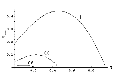
Figure 7: The time duration of GRBs, evaluated in our model with $n=\overline{n}$. It is plotted versus the inclination angle $\theta$ for a number of possible thicknesses $\eta_{{}_{L}}$. As seen, the order of time durations are of the order of ones in short duration GRBs (see § 4.2).

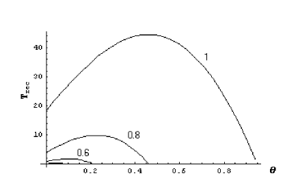
Figure 8: The time duration of GRBs, evaluated in our model with $n=10^{-6}\overline{n}$. It is plotted versus the inclination angle $\theta$ for a number of possible thicknesses $\eta_{{}_{L}}$. As seen, the order of time durations are of the order of ones in long duration GRBs (see § 4.2).

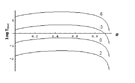
Figure 9: $\log T_{rec}(L;n,\theta)$ is plotted versus the inclination angle $\theta$ for a number of densities, with $\eta_{{}_{L}}\equiv L/l(n/E)$ equal to the highest permitted value $\eta_{m}$. The number near each curve is $\log(n/\overline{n})$ ($\overline{n}=2.9\times 10^{17}cm^{-3}$) (see § 3 and § 4.2 ).

At the mean time the observed bimodality must be interpreted as a result of the second reason expressed in § 4.1. Though in our model one may expect only one heap in the $logT_{\oplus}$ distribution associated with the directions in the clouds having both the most probable $L$ and $n$ (which are equal or near to $\overline{L}$ and $\overline{n}$), but as the numerical computation shows, such directions in the clouds are too thick and too dense to be crossed out by the ejecta, and therefore a real GRB would not be produced. So, we are left with four other regions with high probabilities:
1) $n\sim\overline{n}$ and $L<\overline{L}$ (short GRBs)
2) $n\sim\overline{n}$ and $L>\overline{L}$ (no GRBs)
3) $n>\overline{n}$ and $L\sim\overline{L}$ (no GRBs)
4) $n<\overline{n}$ and $L\sim\overline{L}$ (long GRBs)
Now, we show that the directions trough the clouds associated with region(1) produce the short duration GRBs, and ones associated to regions (2) and (3) produce no GRB, while the others in the forth region produce the long duration ones.
As to the equation(9) the quantity $l(n/E)$ (which is of the order of the sedov length) is $\sim 7\times 10^{11}cm\ll\overline{L}$ for $n\sim\overline{n}$ (see Eqn.[25]). As seen in Fig.7, the time duration of GRBs associated to such directions is of the order of the time duration of short GRBs (Case (1) above). Fig.8 shows that in our model the calculated time duration of GRBs for $n\sim 10^{-6}\overline{n}$ is of the order of the duration of long GRBs. Using equation(9), we see that in this case ( $n\sim 10^{-6}\overline{n}$ ), $l(n/E)$ is about $5\times 10^{13}cm\sim\overline{L}$. So in our model the long duration GRBs are due to the passing of ejecta through the directions where $n\ll\overline{n}$ and $L\sim\overline{L}$ (case (4) above). Furthermore, Since $l(n/E)\ll\overline{L}$ when $n\sim\overline{n}$, we see that in cases (2) and (3) above, the ejecta would stop in the dense cloud and the produced photons can not scape from the optically thick cloud. In Fig.9, $T_{rec}(L;n,\theta)$ is plotted for a number of densities, when $\eta_{{}_{L}}=L/l(n/E)$ has the highest permitted value $\eta_{m}$.
These general features of our calculations result from the general features of our model, and therefore we speculate that any distributions for the clouds thickness and density which are picked around a mean value could explain the general features of the duration distribution. Our chose of gaussian distributions for thickness and density was only for the few parameters needed to describe them.

4.3 The Opacity

In ”The Dense Cloud Model” at this stage we have simply omitted the bursts which ejectas can not go out of the cloud and stop in it (because the emitted photons would be scattered by the dense cloud), and we have claimed that the produced photons by all bursts that succeed to cross out the dense cloud can finally enter the free space.
At the first glance the model might appear to have a serious problem in opacity, namely, in this model the best fit mean density and mean thickness of the clouds are found to be of the orders of $n\sim 10^{17}cm^{-3}$ and $L\sim 10^{13}cm$. So, as to the relation $\tau_{op}=\sigma_{{}_{T}}\>n\>L$, ($\sigma_{{}_{T}}=6.65\times 10^{-25}cm^{2}$) one would expect an optical depth of the order of $10^{6}$. But there are two factors that remedy the situation:
(i) As the numerical calculation shows (see § 4.2), the most probable directions characterized by $n\sim\overline{n}$ and $L\sim\overline{L}$ are dynamically too thick to be crossed out by the ejecta and the radiation produced in this case would be completely scattered by the dense cloud. On the other hand, as discussed in § 4.2, the long duration GRBs are due to the crossing of ejecta through directions where $n\sim 10^{-6}\overline{n}$ and $L\sim\overline{L}$. since the density is reduced by the factor $10^{-6}$, the optical depth drops to the order of $1$. As explained in § 4.2, the short duration GRBs are due to the directions in the cloud where $n\sim\overline{n}$ and $L\sim 10^{-2}\overline{L}$. In this case the optical depth of the cloud reduces to $\sim 10^{4}$, which is yet too high. But,
(ii) most of photons emitted off the shock front have the chance to be overtaken by the moving shock (appendix B). Moreover, it has been shown (Shekh-Momeni & Samimi, 2004) that in high temperatures $kT\sim 10^{6}\>m_{e}c^{2}$ the cross section of Compton scattering for instance for $Mev$ photons effectively drops to $\sim 10^{-6}\>\sigma_{{}_{T}}$, so such a high temperature plasma is much more transparent than what may seem at first. The same is true for the case of a power law distribution of electrons (see Eqn.[A4]). Most of the electrons in such a distribution have energies of the order of $\gamma_{e,min}m_{e}c^{2}\sim 2\times 10^{5}m_{e}c^{2}$, in which we have used equation(A5), taking $p=2.5$, $\xi_{e}=1/3$ and $\Gamma=10^{3}$. For this case the Compton cross section suppresses by the factor of $\sim 10^{-3}-10^{-4}$ for $100ev-1Kev$ photons (the energy of the emitted photons in the shocked medium comoving frame is less than their observed energy by the factor of $\Gamma$), and therefore, the optical depth drops to the order of $1$. So the photons overtaken by the shocked medium may remain in it without being scattered until the shocked medium crosses up the dense cloud. Briefly, due to this second factor, the optical depth in short duration case diminishes to $\tau_{op}\sim 1$, and the optical depth in long duration case diminishes to $\tau_{op}\ll 1$.
The variability seen in the light curves of long duration GRBs maybe attributed to the heterogeny of cloud’s density in the ejecta’s trajectory. This maybe the case in long duration GRBs for which $\tau_{op}\ll 1$, but in short duration GRBs for which $\tau_{op}\sim 1$, we expect that such a heterogeny would not be appeared.
The lateral expansion of the shocked medium can reduce its density and therefore its optical depth. This effect of course may cool the shocked medium and cause an increase in effective Compton cross section in it. The consideration of dynamical feedback makes our modeling much more complicated and it has been neglected here. In ”The Dense Cloud Model” at this stage we have simply omitted the bursts which ejectas can not go out of the cloud and stop in it, but have claimed that the produced photons by all bursts that succeed to cross out the dense cloud can finally enter free space.

A complete study needs to include flux computations. An exact comparison with observed time duration data would be possible only when the theoretical time duration appearing in this work were exactly evaluated in the same manner as the observable duration $T_{90}$ is defined (as the time interval over which $5$ percent to $95$ percent of the burst counts accumulate). Moreover, the BATSE’s triggering mechanism made it less sensitive to short GRBs than to long ones and therefore short GRBs were detected to smaller distances (Mao,Narayan,& Piran, 1994; Cohen & Piran, 1995; Katz & Canel, 1996), so a smaller number of them have been observed. Lee & Petrosian petrosian (1996) studied this effect and corrected the number of short GRBs. In a more exact work this correction must be considered too.

We acknowledge the anonymous referee for valuable comments. F. S. acknowledges Mr. Mehdi Haghighi for his guides on computational methods. This research has been partly supported by Grant No. NRCI 1853 of National Research Council of Islamic Republic of Iran.

Appendix A Scyncrotron Cooling Time in Dense Cloud Model

In this part we use the review paper of Piran (1999) to estimate the synchrotron cooling time in our model. The synchrotron cooling time in the comoving frame is:

$$t_{syn,co}=\frac{3m_{e}c}{4\sigma_{T}U_{{}_{B}}\>\gamma_{e}}~{},$$ (A1)

where $\sigma_{T}$ is the Thompson cross section and $\gamma_{e}$ is the Lorentz factor of the emitting electron, while $U_{{}_{B}}$ stands for the energy density of magnetic field which in GRB literature is assumed to be proportional to $u$, the comoving internal energy density of the shocked matter:

$$U_{{}_{B}}=\xi_{{}_{B}}u~{},$$ (A2)

so that $\xi_{{}_{B}}$ represents the share of magnetic field in $u$, which is given by:

$$u=4\Gamma^{2}nm_{p}c^{2}~{},$$ (A3)

in which, $n$ is the number density of surrounding medium (ISM, or a dense cloud as assumed in our model), and $\Gamma$ denotes the Lorentz factor of the shocked matter.
The electrons in shocked media are assumed to develop a power law distribution of Lorentz factors:

$$N(\gamma_{e})\propto\gamma_{e}^{-p}\>\>\>\>\>\>\>\>\>\>\>\>\>for:\>\>\>\>\>\>\>\>\>\>\>\gamma_{e}>\gamma_{e,min}~{}.$$ (A4)

The convergence of total energy of the electrons requires the power index $p$ to be greater than $2$, while the assumed lower limit $\gamma_{e,min}$ is to prevent the divergence of electron number density and is obtained to be:

$$\gamma_{e,min}=\frac{m_{p}}{m_{e}}\>\frac{p-2}{p-1}\>\xi_{e}\>\Gamma~{},$$ (A5)

where $\xi_{e}\equiv u_{e}/u$ represents the share of the electrons in the internal energy of shocked matter.
Furthermore, the time interval between emission of two photons from the same point in the comoving frame, $\delta t_{co}$, and the time interval $\delta t_{\oplus}$, which represents the time interval of their successive arrival to a cosmologically distant observer (at the earth), are related as below:

$$\delta t_{\oplus}=(1+z)\frac{\delta t_{co}}{2\Gamma}~{}.$$ (A6)

Equations(A1-A6) are adopted from Piran (1999). Now, by substituting equations(A2),(A3), & (A5) in equation(A1), and then using equation(A6), the synchrotron cooling time measured by a terrestrial observer turns out to be:

$$t_{syn,\oplus}<\frac{3}{32}(1+z)\xi_{e}^{-1}\xi_{B}^{-1}\left(\frac{m_{e}}{m_{p}}\right)^{2}\left(\frac{p-1}{p-2}\right)(\sigma_{{{}^{T}}}nc)^{-1}\Gamma^{-4}sec$$

$$\sim 10^{-12}(1+z)\left(\frac{\xi_{e}}{0.1}\right)^{-1}\left(\frac{\xi_{B}}{0.1}\right)^{-1}\left(\frac{n}{10^{18}}\right)^{-1}\Gamma^{-4}sec~{},$$ (A7)

which is clearly much less than all observed time durations of GRBs. So, the synchrotron emission in a dense cloud model must be considered as an instantaneous process, and therefore the shock front must be regarded as the emitting surface. This allows us to attribute time duration of a GRB merely to the time that the shock front takes to cross the dense cloud.

Appendix B The relation between Lorentz factors of the shocked matter and the emitting surface

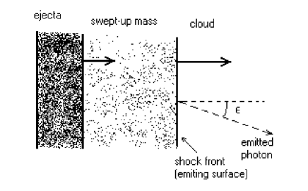
Figure 10: The shocked matter and the shock front (emitting surface) speeds, as viewed in the source frame. In the figure, if the angle $\epsilon$ were larger than $1/\Gamma^{\prime}$ the photon would be overtaken by the shock front (from which it were emitted), so that the photon would remain in the shocked medium (see appendix B).

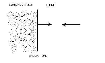
Figure 11: The shock front (emitting surface) speed $\beta^{\prime}_{co}$, measured in the shocked frame. In this frame the cloud has a density of $\Gamma n$ and moves toward the shocked medium with a speed $\beta$, and becomes compressed to a density of $4\Gamma n$. So clearly we have $\beta^{\prime}_{co}=\beta/4$ (see appendix B).

Here, we want to find the relation between $\Gamma$ and $\Gamma^{\prime}$ which are respectively the Lorentz factors of the shocked matter and of the shock front (which is the emitting surface in our model; see appendix A). In Fig.10, $\beta$ and $\beta^{\prime}$ correspond to shocked matter and shock front speeds, both measured in the (central) source frame. In the shocked matter frame (Fig.11) the dense cloud which is seen to have a density $\Gamma\>n$, moves toward the shocked medium with a speed $\beta$, while being compressed to a density equal to $4\Gamma n$. Consequently, as illustrated in Fig.11, the shocked medium expands towards right with a speed $\beta^{\prime}_{co}$ which is in fact the speed of the shock front in the shocked matter frame (compare Fig.10 and Fig.11). Considering the conservation of nucleon number, it is seen that:

$$\beta^{\prime}_{co}=\frac{\beta}{4}~{}.$$ (B1)

Considering the relativistic summation of velocities, we have:

$$\beta^{\prime}=\frac{\beta^{\prime}_{co}+\beta}{1+\beta\beta^{\prime}_{co}}~{}.$$ (B2)

Noting the relations $\Gamma=(1-\beta^{2})^{-1/2}$ and $\Gamma^{\prime}=(1-{\beta^{\prime}}^{2})^{-1/2}$, the substitution of equation(B1) in equation(B2) finally yields:

$$\Gamma^{\prime}\simeq\sqrt{\frac{5}{3}}\>\>\Gamma~{},$$ (B3)

The distance from the origin to the shock front, denoted by $r^{\prime}$, can be obtained by integrating $\beta^{\prime}$ over $t$:

$$r^{\prime}=\int_{0}^{t}\beta^{\prime}\>cdt\>+r_{0}~{}.$$ (B4)

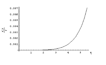
Figure 12: $(r^{\prime}-r)/r$ versus $\eta\equiv r/l(n/E)$, with $n=2.9\times 10^{17}cm^{-3}$ (see appendix B).

The results are shown in Fig.12. As seen, the difference between $r$ and $r^{\prime}$ never exceeds one percent. This result justifies the use of symbol $r$ (instead of $r^{\prime}$ )for the location of the shock front through out our formulation.
Now, let’s consider a photon that is radiated from the shock front (the emitting surface) moving with the Lorentz factor $\Gamma^{\prime}$ (Eqn.[B3]), in a direction which makes an angle $\epsilon$ with the velocity vector of the shocked matter (Fig.10). if :

$$\epsilon>\Gamma^{\prime-1},$$ (B5)

the photon would be overtaken by the shock front. The majority of the emitted photons fulfill this condition when $\Gamma^{\prime}\sim 10^{3}$ and $\zeta_{0}\sim 10^{-2}$ (see Eqn.[25]).

Appendix C Geometrical Considerations

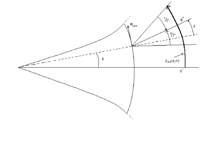
Figure 13: Geometry of Radiation. The lateral speed of the emitting segment, $v_{lat}$, causes the radiation cone axis $z^{\prime\prime}$ to make an angle $\epsilon+\delta$ with $z^{\prime}$ axis, where $\delta=\tan^{-1}[\epsilon c_{s}/(\Gamma\beta c\zeta)]$ (see appendix C).

Here the effect of burster geometry on the observed time duration is investigated. At first, as shown in Fig.13, we consider a radiating segment on the shock front. The symmetry axis is denoted by $z^{\prime}$. Noting the definition of $\epsilon$ in the figure, it is seen that in addition to a radial component $dr/dt$, the velocity vector of the segment must have a lateral component $v_{lat}$ which is equal to:

$$v_{lat}=\frac{\epsilon}{\Gamma(\eta)\zeta(\eta)}~{}c_{s}~{},$$ (C1)

as measured in the source frame. In equation(C1) the non-dimensional radius $\eta$, as defined in equation(8), is used instead of $r$, . Equation(C1) is obtained simply by using equation(5) and assuming that the lateral speed of the segment in a frame moving (only radially and) instantaneously along with the segment, is the fraction $\epsilon/\zeta(\eta)$ of sound speed $c_{s}$ (which is the lateral speed of the emitting surface at its edges), and noting that the lateral speed in the source frame is less than its corresponding value in the (radially instantaneous) comoving frame by the factor $1/\Gamma$. It is well known that the radiation emitted by the segment is almost confined to an angle $1/\Gamma$. In Fig.13 the axis of the radiation cone emitted by the segment is denoted by $z^{\prime\prime}$, which is parallel to the velocity vector of the segment and, as seen in the figure, makes an angle $\epsilon+\delta$ with $z^{\prime}$ axis, where $\delta=\tan^{-1}[\epsilon c_{s}/(\Gamma\beta c\zeta)]$. So the radiation angle $\zeta_{rad}(\eta,\epsilon)$ (as depicted in the figure) can be written as below:

$$\zeta_{rad}(\eta,\epsilon)=\epsilon+\tan^{-1}\left(\frac{\epsilon\>c_{s}/c}{\Gamma(\eta)\>\beta(\eta)\>\zeta(\eta)}\right)+1/\Gamma(\eta)~{},$$ (C2)

and the total radiation angle, defined as the radiation angle at the edge of the emitting surface, can be written as:

$$\zeta_{rad}(\eta)\equiv\zeta_{rad}(\eta,\epsilon=\zeta(\eta))=\zeta(\eta)+\tan^{-1}\left(\frac{c_{s}/c}{\Gamma(\eta)\>\beta(\eta)\>}\right)+1/\Gamma(\eta)~{}.$$ (C3)

This angle represents the cone of space illuminated by the emitting surface. Using the results of equation(7), the total radiation angle can be evaluated for every ”$\eta$”. Having defined the total radiation angle, we explore the effect of burster geometry on its observed time duration $T_{\oplus}$. As shown in Fig.2, the problem is studied in a spherical coordinate system in which the central engine is taken as the origin, and the line-of-sight as the polar axis $z$. Consider a photon emitted off a point on the emitting surface (the shock front) with radial coordinate $r$ and polar coordinate $\Theta$; and at an instance t, measured in the source frame (the point is not shown in the figure). The relation between $t$ and the photon arrival time $t_{rec}$ to a (cosmologically) near observer is obtained by Granot, Piran, & Sari granot (1999). Making suitable for our model, it is adjusted to the form below:

$$t_{rec}=t-\frac{r\>\cos\Theta-r_{0}}{c}~{}.$$ (C4)

In this equation the instance $t=0$ is defined as the time that the ejecta collides with the dense cloud at $r=r_{0}$; while $t_{rec}=0$ is the time that the (cosmologically) near observer receives the photon emitted at $t=0$ from the point with coordinates $r=r_{0}$ and $\Theta=0$. Defining:

$$\tau_{rec}\equiv\frac{c\>t_{rec}}{l(n/E)}~{},$$ (C5)

and noting equation(8) and equation(12), we rewrite equation(C4) in the form below:

$$\tau_{rec}=\tau-\eta\>\cos\Theta+\eta_{0}~{}.$$ (C6)

Multiplying equation(C4) by the cosmological time dilation term $(1+z)$, results in the arrival time as maybe observed at the earth:

$$t_{\oplus}=(1+z)t_{rec}=(1+z)\left(t-\frac{r\>\cos\Theta-r_{0}}{c}\right)~{},$$ (C7)

or equivalently:

$$\tau_{\oplus}=(1+z)\tau_{rec}=(1+z)(\tau-\eta\>\cos\Theta+\eta_{0})~{},$$ (C8)

in which we used the non-dimensional time duration $\tau_{\oplus}$ defined as below:

$$\tau_{\oplus}\equiv\frac{c\>t_{\oplus}}{l(n/E)}~{}.$$ (C9)

Now, as shown in Fig.2, we consider a situation where the ejecta’s symmetry axes makes an angle $\theta$ with the line of sight. The necessary condition that at least some photons of the emitting surface are detected by the near observer is:

$$\zeta_{rad}(\eta)>\theta~{}.$$ (C10)

Here we denote the inverse of function $\zeta_{rad}(\eta)$ by $\eta_{rad}(\zeta_{rad})$, which gives the radius corresponding to $\zeta_{rad}$. As seen in Fig.2, for $\theta$’s larger than $\zeta_{rad}(\eta_{0})$, the first photons reaching the detectors are those emitted at $\eta=\eta_{rad}(\theta)$. So, we use $\tau(\eta)$ (which is obtainable by solving equation(11)) to write:

$$\tau_{1}(\theta)=\cases{0&\mbox{i}f $\>\>\>\>\>\theta<\zeta_{rad}(\eta_{0})$\cr\tau(\eta_{rad}(\theta))&\mbox{i}f$\>\>\>\>\>\>\theta>\zeta_{rad}(\eta_{0})$},$$ (C11)

where $\tau_{1}(\theta)$ represents the starting time (in the source frame) that the emitted photons can reach the (cosmologicaly near) observer. Now, using the numerical results of equation(11) we can obtain the function $\eta(\tau)$. Then, considering equation(C6), the non-dimensional time $\tau_{rec,1}(\theta)$ corresponding to $\tau_{1}(\theta)$ would be as below:

$$\tau_{rec,1}(\theta)=\cases{0&\mbox{:}$\>\>\theta<\zeta_{0}$\cr-\eta_{0}\cos(\theta-\zeta_{0})+\eta_{0}&\mbox{:}$\>\>\zeta_{0}<\theta<\zeta_{rad}(\eta_{0})$\cr\tau(\eta_{rad}(\theta))-\eta_{rad}(\theta)\cos[\theta-\zeta(\eta_{rad}(\theta))]+\eta_{0}&\mbox{:}$\>\>\theta>\zeta_{rad}(\eta_{0})$}~{}.$$ (C12)

Now, we are to find the time $\tau_{rec,2}(\theta)$ after which no photons can be detected by the near observer. In Fig.2, the photons emitted from the edge point $A$ can reach us at all times greater than $\tau_{1}(\theta)$. Let’s remind that in our model the emission process terminates at the time that the shocked matter goes out of the cloud (appendix A). As is seen in equation(C6), the closer to the point $B$ is a point on the emitting surface, the later its emitted photons would reach the near observer, of course, provided that the observer line-of-sight remains in the radiation cone of the emitting point.
Defining:

$$\eta_{L}\equiv\frac{r_{0}+L}{l(n/E)}~{},$$ (C13)

and recalling equation(C2), we can solve the equation:

$$\zeta_{rad}(\eta_{{}_{L}},\epsilon)=\theta~{},$$ (C14)

to find the function $\epsilon=\epsilon(\eta_{{}_{L}},\theta)$, which specifies the furthest point (on the shock front at the radius $\eta_{{}_{L}}$) which its radiation reaches us, of course, if it remains smaller than $\zeta(\eta_{{}_{L}})$.
Now, using equation(C6), we can find the instance that the last photons reach the near observer:

$$\tau_{rec,2}(\theta,\eta_{{}_{L}},\eta_{0})=\tau(\eta_{{}_{L}})-\eta_{{}_{L}}\>\cos(\theta+min[\epsilon(\eta_{{}_{L}},\theta),\zeta(\eta_{{}_{L}})])+\eta_{0}~{}.$$ (C15)

Finally, the non-dimensional time duration of a GRB, $\tau_{rec}(\theta,\eta_{{}_{L}})$, will be equal to $\tau_{rec,2}(\theta,\eta_{{}_{L}})-\tau_{rec,1}(\theta)$ and, as to equation(C12) and equation(C15), besides being a function of parameters of the ejecta and the cloud, it is also a function of the inclination angle $\theta$. So, the time duration of a GRB as measured by an observer cosmologivally near to it would be a function of $L$, $n$, and $\theta$:

$$T_{rec}=T_{rec}(L;n,\theta)~{},$$ (C16)

where:

$$T_{rec}=\tau_{rec}(\theta,\eta_{{}_{L}})\frac{l\left(n/E\right)}{c},$$ (C17)

The expression(C16) needs some explanations. In our model the ejecta parameters $\zeta_{0}$ , $E$ and $\Gamma_{0}$ and the radius $r_{0}$ are assumed to be the same in all GRBs. So, these parameters do not appear in equation(C16) explicitly , though it is implicitly a function of them too. At the mean time, the cloud’s density $n$ and its thickness $L$ are assumed to be different in different directions, and therefore they do appear explicitly in the expression (C16). Furthermore, if a cloud thickness $L$ is much more than its associated $Sedov$ length $l_{sedov}\equiv(E/n\>m_{p}\>c^{2})^{1/3}$, the ejecta may not cross it up, and finally stops in it. In such a situation the time duration of a GRB would not be a function of $L$, while it still remains dependent on $n$ and $\theta$. This is why in expression (C16), the quantity $L$ is distinguished from $n$ and $\theta$ by a semicolon. The rearrangement of the expression(C16) in the form $L=L(T_{rec},)\theta,n$ would be meaningful only when we are dealt with the situation where the ejecta succeed to cross up the cloud (see Eqn.[15]).

Appendix D The explicit form of $F_{{}_{GRB}}(z)$

Here the relation between $F_{{}_{GRB}}(z)$ appearing in equation(23) and the GRB occurring rate $f_{{}_{GRB}}(z)$ (in units of $Mpc^{-3}\>yr^{-1}$) is derived, so that by adopting a cosmological model for the occurring rate, the integral in equation(23) can be evaluated.
The number of GRBs that their effects could reach us in a time interval $\delta t_{0}$ (which is very much less than the present comoving time $t_{0}$), and from a spherical volume element $\delta V_{z}$ (disregarding various effects, such as the geometrical ones discussed in appendix C, or those related to detectors threshold which affect the number of detected GRBs) is as below:

$$\delta^{2}N_{{}_{GRB}}=f_{{}_{GRB}}(z)\>\delta V_{z}\>\>\frac{\delta t_{0}}{1+z}$$

$$=f_{{}_{GRB}}(z).\>4\pi R^{{}^{3}}(z)\>r^{{}^{2}}(z)\>\delta r(z)\>\frac{\delta t_{0}}{1+z}~{},$$ (D1)

where $r(z)$ denotes the non-dimensional radial parameter of the source that its effects reach us with a red shift z, and $R(z)$, the scale factor at this red shift. In Einstein-de Sitter model we have:

$$R_{0}\>r(z)=\frac{2c}{H_{0}}\{1-(1+z)^{-1/2}\}~{},$$ (D2)

where $H_{0}$ is the Hubble constant. Furthermore, in FRW metrics:

$$R(z)=R_{0}(1+z)^{-1}~{},$$ (D3)

where $R_{0}\equiv R(z=0)$. Now, using equations(D2) and (D3) in equation(D1) we obtain:

$$F_{{}_{GRB}}(z)\propto\frac{\delta^{2}N_{{}_{GRB}}}{\delta t_{0}\delta z}=2\pi\>\left(\frac{2c}{H_{0}}\right)^{{}^{3}}(1+z)^{{}^{-11/2}}\>\{1-(1+z)^{-1/2}\}^{{}^{2}}\>f_{{}_{GRB}}(z)~{}.$$ (D4)

What is remained is the explicit form of $f_{{}_{GRB}}(z)$. The high variability seen in GRB light curves has convinced the investigators to relate GRBs to stellar objects , and consequently their rate $f_{{}_{GRB}}(z)$ to the star formation rate $f_{{}_{SF}}(z)$. The simplest model is of course a proportional model $f_{{}_{GRB}}(z)\propto f_{{}_{SF}}(z)$. the proportional model may be correct if GRBs are attributed to the evolution of massive stars whose lifetime is negligible in comparison with the cosmological time scale, but in NS-NS mergers model the proportionality may not be valid (because of the delay time from the star formation to NS-NS mergers). Wijers et al. wijers (1998) claimed that there is a good consistency between the proportional model and the observed GRB brightness distribution, while Petrosian & Lloyd petrosian2 (1998) concluded that none of the NS-NS and the proportional model are in agreement with the observed $f_{{}_{SF}}(z)$. Totani totani (1999) ascribed this discrepancy to the uncertainties in SFR observations. Anyway we simply assume the GRB rate to be as below:

$$f_{{}_{GRB}}(z)=f_{{}_{GRB}}(0)(1+z)^{{}^{3+q}}~{},$$ (D5)

and treat $q$ as a free parameter that its best value should be obtained during the fitting procedure. In Fig.14, $F_{{}_{GRB}}(z)$ is plotted for a number of $q$’s. Clearly the case $q=0$ corresponds to a universe where the changes in the rates of astrophysical phenomena are only due to its expansion (non-evolutionary universe). It can be seen that $F_{{}_{GRB}}(z)$ takes its maximum at $z\sim 1$, which is not very sensitive to the magnitude of $q$.

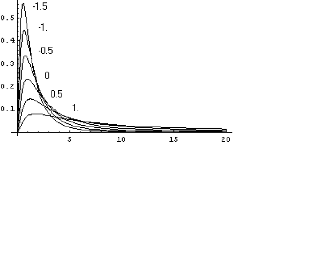
Figure 14: The quantity $F_{{}_{GRB}}(z)$ (the probability density of observing a GRB at a redshift $z$) is plotted for a number of $q$’s (the value of $q$ is written near to the peak of its corresponding curve). As seen, all curves have a maximum at $z\sim 1$. This explains why the most of GRBs have redshifts $z\sim 1$ (see Eqn.[D5]).

References

- Akerlof et al. (2003) Akerlof, C. W., et al. 2003, PASP, 115, 132A
- Begelman,Blandford,&Rees (1984) Begelman, M. C., Blandford, R. G., & Rees, M. J. 1984, Reviwes of Modern Physics, 56, 255
- Cohen & Piran (1995) Cohen, E. & Piran, T. 1995, ApJ, 444, L25
- Costa et al. (1997) Costa, E., et al. 1997, Nature, 387, 783
- Dingus et al. (1993) Dingus, B. L., et al. 1993, AAS, 182, 7404
- Fishman et al. (1993) Fishman, G. J., et al. 1993, A&AS, 97, 17
- Frail et al. (1997) Frail, D., Kulkarni, S. R., Nicastro, S. R., Feroci, M., Taylor, G. B. 1997, Nature, 389, 261
- Gisler et al. (1999) Gisler, G. R., et al. 1999, in AIP Conf. 499, Small Missions for Energetic Astrophysics : Ultraviolet to Gamma-Ray, ed. S. P. Brumby & N.Y. Melville (AIP), 82
- (9) Granot, J., Piran, T., & Sari, R. 1999, ApJ, 513, 679
- Granot (2003) Granot, J. 2003, ApJ, 596, L17
- Jones et al. (1996) Jones, B. B., et al. 1996, ApJ, 463, 565
- (12) Katz, J. I. 2002, The Biggest Bangs (Oxford U.Press)
- Katz & Canel (1996) Katz, J. I., & Canel, L. M. 1996, ApJ, 471, 915
- (14) Katz, J. I. 1994, ApJ, 432, L27
- Kouveliotou et al. (1993) Kouveliotou, C., et al. 1993, ApJ, 413, L101
- Kulkarni et al. (1999) Kulkarni, S. R.,et al. 1999, Nature, 398, 389
- Lamb,Donaghy,& Graziani (2004) Lamb, D. Q., Donaghy, T. Q., Graziani, C. 2004, NewAR, 48, 459
- (18) Lee, T. T., & Petrosian, V. 1996, ApJ, 470, L479
- Mao,Narayan,& Piran (1994) Mao, S., Narayan, R., & Piran, T. 1994, ApJ, 420, 171
- Meegan et al. (1996) Meegan, C. A., et al. 1996, ApJS, 106, 65
- Norris et al. (1993) Norris, J. P., Nemiroff, R. J., Kouveliotou, C., Fishman, G. J., Meegan, C. A., & Paciesas, W. S. 1993, AAS, 183, 2904
- Paciesas et al. (1999) Paciesas, W. S., et al. 1999, ApJS, 122, 465
- (23) Paczynski, B., & Rhoads, J. E. 1993, ApJ, 418, L5
- (24) Petrosian, V., Lloyd, N. M. 1998, in AIP Conf. 428, Gamma-Ray Bursts, ed. C. A. Meegan, R. D. Preece, & T. M. Koshut (AIP), 35
- piran (1999) Piran, T. 1999, PhR, 314, 575
- (26) Podsiadlowski, P., Cannon, R. C., Rees, M. J. 1995, MNRAS, 274, 485
- (27) Qin, B., Wu, X., Chu, M., Fang, L., & Hu, J. 1998, ApJ, 494, L57
- (28) Rhoads, J. E. 1999, ApJ, 525, 737
- Shekh-Momeni & Samimi (2004) Shekh-Momeni, F., & Samimi, J. 2004, preprint (astro-ph/0402194)
- (30) Terman, J. L., Taam, R. E., Hernquist, L. 1995, ApJ, 445, 367
- Thorne & Zytkow (1977) Thorne, K. S., & Zytkow, A. N. 1977, ApJ, 212, 832
- (32) Totani, T. 1999, ApJ, 511, 41
- van Paradijs et al. (1997) van Paradijs, J., et al. 1997, Nature, 386, 686
- Waxman (2003) Waxman, E. 2003, Nature, 423, 388
- (35) Wijers, R. M. J., Bloom, J. S., Bagla, J. S., Natarajan, P. 1998, MNRAS, 294, L13
- Yu et al. (1998) Yu, W., Li, T., Wu, M. 1998, tx19.confE, 90Y (astro-ph/9903126)