Propagation of Electromagnetic Waves on
a Rectangular Lattice of Polarizable Points

Abstract

We discuss the propagation of electromagnetic waves on a rectangular lattice of polarizable point dipoles. For wavelengths long compared to the lattice spacing, we obtain the dispersion relation in terms of the lattice spacing and the dipole polarizabilities. We also obtain the dipole polarizabilities required for the lattice to have the same dispersion relation as a continuum medium of given refractive index $m$; our result differs from previous work by Draine & Goodman (1993). Our new prescription can be used to assign dipole polarizabilities when the discrete dipole approximation is used to study scattering by finite targets. Results are shown for selected cases.

1 Introduction

The discrete dipole approximation (DDA) provides a flexible and general method to calculate scattering and absorption of light by objects of arbitrary geometry (Draine, 1988; Draine & Flatau, 1994). The approximation consists of replacing the continuum target of interest by an array of polarizable points, which acquire oscillating electric dipole moments in response to the electric field due to the incident wave plus all of the other dipoles. Broadly speaking, there are two criteria determining the accuracy of the approximation:

• the interdipole separation $d$ should be small compared to the wavelength of the radiation in the material ($|m|kd<1$, where $m$ is the complex refractive index, and $k=\omega/c$ is the wavenumber in vacuo);

• the interdipole separation $d$ should be small enough to resolve structural dimensions in the target.

With modern workstations, it is now feasible to carry out DDA calculations on targets containing up to $\sim 10^{6}$ dipoles (Draine & Flatau, 1994). In addition to calculation of scattering and absorption cross sections, the DDA has recently been applied to computation of forces and torques on illuminated particles (Draine & Weingartner, 1996, 1997)

If the dipoles are located on a cubic lattice, then in the limit where the interdipole separation $kd\rightarrow 0$, the familiar Clausius-Mossotti relation (see, e.g, Jackson (1962)) can be used to determine the choice of dipole polarizabilities required so that the dipole array will approximate a continuum target with dielectric constant $\epsilon$. Draine (1988) showed how this estimate for the dipole polarizabilities should be modified to include radiative reaction corrections, and Draine & Goodman (1993) derived the $O[(kd)^{2}]$ corrections required so that an infinite cubic lattice would have the same dispersion relation as a continuum of given dielectric constant.

Nearly all DDA calculations to date have assumed the dipoles to be located on a cubic lattice. If, instead, a rectangular lattice is used, it will still be possible to apply FFT techniques to the discrete dipole approximation, in essentially the same way as has been done for a cubic lattice (Goodman, Draine & Flatau, 1991). However, the ability to use different lattice constants in different directions might be useful in representing certain target geometries.

The objective of the present report is to obtain the dispersion relation for propagation of electromagnetic waves on a rectangular lattice of polarizable points. This dispersion relation will be expanded in powers of $(kd)$, where $d$ is the characteristic interdipole separation. For a lattice of specified dipole polarizabilities, this will allow us to determine the dispersion relation for electromagnetic waves propagating on the lattice when $(kd)^{2}\ll 1$. Alternatively, if we require the lattice to propagate waves with a particular dispersion relation, inversion of the lattice dispersion relation will provide a prescription for assigning dipole polarizabilities when seeking to approximate a continuum material with a rectangular lattice of polarizable points.

2 Mode Equation for a Rectangular Lattice

The problem of wave propagation on an infinite polarizable cubic lattice of point dipoles has been solved previously by Draine & Goodman (1993, herafter DG93). Here we describe the generalization of this problem to rectangular lattices.

Consider an infinite rectangular lattice with lattice sites at

$${\bf x}_{\bf n}=(n_{1}d_{1},n_{2}d_{2},n_{3}d_{3})\,,$$ (1)

where the $n_{i}$ are integers and the lattice constants $d_{i}$ are, in general, all different. The density $n$ of dipoles is just

$$n={1\over d_{1}d_{2}d_{3}}~{}~{}~{},$$ (2)

and it will be convenient to define the characteristic lattice length scale

$$d\equiv(d_{1}d_{2}d_{3})^{1/3}~{}~{}~{}.$$ (3)

Since the lattice is anisotropic, the polarizability ff of the dipoles located at lattice sites is a tensor, i.e., the polarization is

$${\bf P}({\bf x})={\hbox{\boldsym\char 11\relax}}\cdot{\bf E}({\bf x})\,.$$ (4)

Thus the polarization vector is not, in general, parallel to the electric field or to the vector potential. From charge conservation we have

$$\nabla\cdot{\bf J}=0\,,$$ (5)

or, since

$${\bf J}={\partial{\bf P}\over\partial t}\,,$$ (6)

we obtain the transversality condition

$$\nabla\cdot{\bf P}=0\,.$$ (7)

We assume that the dipole moment at the lattice site ${\bf x}_{\bf n}$ is

$${\bf P}_{\bf n}(t)={\bf P}_{0}(0)e^{i{\bf k}\cdot{\bf x}_{\bf n}-i\omega t}\,.$$ (8)

With the Lorentz gauge condition

$$\nabla\cdot{\bf A}+{1\over c}{\partial\Phi\over\partial t}=0$$ (9)

and equation (6), the vector potential ${\bf A}({\bf x},t)$ satisfies the wave equation

$$\nabla^{2}{\bf A}+{\omega^{2}\over c^{2}}{\bf A} = -{4\pi\over c}{\bf J}$$ (10)

$$= {4\pi i\omega\over c}\sum_{{\bf n}}{\bf P}_{{\bf n}}\delta^{3}({\bf x}-{\bf x}_{\bf n})$$ (11)

$$= {4\pi i\omega\over c}{\bf P}_{0}e^{i{\bf k}\cdot{\bf x}}\sum_{{\bf n}}\delta^{3}({\bf x}-{\bf x}_{\bf n})~{}~{}~{}~{}~{}.$$ (12)

Consider now the unit cell centered on ${\bf x}=0$. Let ${\bf A}_{other}$ and $\Phi_{other}$ be the potentials in this region due to all dipoles except the dipole at ${\bf x}=0$. Thus

$${\bf E}_{other}({\bf x},t)=-{1\over c}{\partial{\bf A}_{other}\over\partial t}-\nabla\Phi_{other}={i\omega\over c}{\bf A}_{1}({\bf x},t)$$ (13)

where

$${\bf A}_{1}({\bf x},t)\equiv{\bf A}_{other}+{c^{2}\over\omega^{2}}\nabla(\nabla\cdot{\bf A}_{other})~{}~{}~{}~{}.$$ (14)

Thus

$${\bf P}_{0}(0)={i\omega\over c}\,{\hbox{\boldsym\char 11\relax}}\cdot{\bf A}_{1}({\bf x}=0,t=0)~{}~{}~{}~{}.$$ (15)

The vector potential can be written

$${\bf A}({\bf x},t)=e^{i{\bf k}\cdot{\bf x}-i\omega t}\sum_{{\bf n}}{\bf a}_{{\bf n}}e^{i{\bf q}\cdot{\bf x}}$$ (16)

where

$${\bf q}\equiv{\bf q}({\bf n})=2\pi\,\bigg{(}{n_{1}\over d_{1}},{n_{2}\over d_{2}},{n_{3}\over d_{3}}\bigg{)}$$ (17)

define a lattice which is reciprocal (e.g., Ashcroft & Mermin (1976)) to the original rectangular lattice on which the dipoles are located. Equations (12) and (16), and the identity

$$\sum_{{\bf n}}\delta^{3}({\bf x}-{\bf x}_{\bf n})={1\over d_{1}d_{2}d_{3}}\sum_{{\bf n}}e^{i{\bf q}\cdot{\bf x}}$$ (18)

yield

$${\bf a}_{{\bf n}}={4\pi\omega^{2}\over c^{2}}\,{1\over d_{1}d_{2}d_{3}}\,{\hbox{\boldsym\char 11\relax}}\cdot{\bf A}_{1}(0,0)\left[|{\bf k}+{\bf q}|^{2}-{\omega^{2}\over c^{2}}\right]^{-1}~{}~{}~{}~{}.$$ (19)

The field ${\bf A}_{self}({\bf x},t)$ due to the dipole at ${\bf x}=0$ is

$${\bf A}_{self}({\bf x},t)={-i\omega\over c}{\bf P}_{0}{e^{i\omega r/c}\over r}={\omega^{2}\over c^{2}}\,{\hbox{\boldsym\char 11\relax}}\cdot{\bf A}_{1}(0,0){e^{i\omega r/c}\over r}e^{-i\omega t}~{}~{}~{}~{}.$$ (20)

With the identity

$${e^{i\omega r/c}\over r}={e^{i{\bf k}\cdot{\bf x}}\over 2\pi^{2}}\int d^{3}k^{\prime}{e^{i{\bf k}^{\prime}\cdot{\bf x}}\over|{\bf k}^{\prime}+{\bf k}|^{2}-\omega^{2}/c^{2}}$$ (21)

we obtain

$${\bf A}_{other}={4\pi\omega^{2}\over c^{2}}{1\over d_{1}d_{2}d_{3}}\,e^{i{\bf k}\cdot{\bf x}-i\omega t}\,{\hbox{\boldsym\char 11\relax}}\cdot{\bf A}_{1}(0,0)\bigg{[}\sum_{\bf n}{e^{i{\bf q}\cdot{\bf x}}\over|{\bf k}+{\bf q}|^{2}-\omega^{2}/c^{2}}~{}-$$

$${d_{1}d_{2}d_{3}\over 8\pi^{3}}\int{d^{3}k^{\prime}}{e^{i{\bf k}^{\prime}\cdot{\bf x}}\over|{\bf k}+{\bf k}^{\prime}|^{2}-\omega^{2}/c^{2}}\bigg{]}~{}~{}~{}.$$ (22)

We seek ${\bf A}_{1}$. Substituting (22) into (14), we obtain after some algebra:

$$A_{1,i}({\bf x},t)={4\pi\over d_{1}d_{2}d_{3}}\sum_{j=1}^{3}\sum_{l=1}^{3}\biggl{[}\sum_{\bf n}\left({\omega^{2}\over c^{2}}\delta_{il}-(k_{i}+q_{i})(k_{l}+q_{l})\right){e^{i({\bf k}+{\bf q})\cdot{\bf x}}\over|{\bf k}+{\bf q}|^{2}-\omega^{2}/c^{2}}~{}-$$

$${d_{1}d_{2}d_{3}\over 8\pi^{3}}\int{d^{3}k^{\prime}}\left({\omega^{2}\over c^{2}}\delta_{il}-(k_{i}+k_{i}^{\prime})(k_{l}+k_{l}^{\prime})\right){e^{i({\bf k}+{\bf k}^{\prime})\cdot{\bf x}}\over|{\bf k}+{\bf k}^{\prime}|^{2}-\omega^{2}/c^{2}}\biggr{]}e^{-i\omega t}\,\alpha_{lj}A_{1,j}(0,0)\,.$$ (23)

For ${\bf x}=0$ and $t=0$ and given values of $\alpha_{ij}$, equation (23) is the mode equation, i.e., it allows determination of the dispersion relation ${\bf k}={\bf k}(\omega)$. However, in the present case, we know the dispersion relation, and wish to determine values of $\alpha_{ij}$ such that the known dispersion relation and equation (23) are satisfied simultaneously. Another relation that must be satisfied follows from (7), (8), (15), and (18):

$${\bf k}\cdot{\bf P}_{0}(0)={\bf k}\cdot{\hbox{\boldsym\char 11\relax}}\cdot{\bf A}_{1}(0,0)=0\,.$$ (24)

Hence, if ${\bf e}$ is a unit vector in the direction of ${\bf A}_{1}$, then

$$\sum_{j=1}^{3}\sum_{l=1}^{3}k_{l}\,\alpha_{lj}\,e_{j}=0\,.$$ (25)

At this point it is convenient to define the following dimensionless quantities:

$$\tilde{q}\equiv{2\pi\over d}={2\pi\over(d_{1}d_{2}d_{3})^{1/3}}$$ (26)

$$\nu\equiv{\omega\over\tilde{q}c}\,;$$ (27)

$${\hbox{\boldsym\char 12\relax}}\equiv{{\bf k}\over\tilde{q}}\,;$$ (28)

$${\hbox{\boldsym\char 13\relax}}\equiv{4\pi\over d_{1}d_{2}d_{3}}\,{\hbox{\boldsym\char 11\relax}}\,;$$ (29)

$${\bf Q}\equiv{{\bf q}\over\tilde{q}}=(n_{1}{d\over d_{1}},n_{2}{d\over d_{2}},n_{3}{d\over d_{3}})\,,$$ (30)

The vectors ${\bf Q}$ define a reciprocal lattice (e.g., Ashcroft & Mermin (1976)).

Using these dimensionless quantities, the mode equation (23) may be written

$$\sum_{j=1}^{3}\sum_{l=1}^{3}M_{il}\,\gamma_{lj}\,e_{j}=e_{i}\,,$$ (31)

where

$$M_{ij}\equiv\sum_{\bf n}{\nu^{2}\delta_{ij}-(\beta_{i}+Q_{i})(\beta_{j}+Q_{j})\over|{\hbox{\boldsym\char 12\relax}}+{\bf Q}|^{2}-\nu^{2}}-\int d^{3}{\hbox{\boldsym\char 12\relax}}^{\prime}{\nu^{2}\delta_{ij}-(\beta_{i}+\beta_{i}^{\prime})(\beta_{j}+\beta_{j}^{\prime})\over|{\hbox{\boldsym\char 12\relax}}+{\hbox{\boldsym\char 12\relax}}^{\prime}|^{2}-\nu^{2}}~{}~{}~{},$$ (32)

and equation (25) becomes

$$\sum_{i=1}^{3}\sum_{j=1}^{3}\beta_{i}\,\gamma_{ij}\,e_{j}=0\,.$$ (33)

It should be noted that the mode equation for a cubic lattice has the same form as equation (31). The matrix elements $M_{ij}$ in equation (32) also have the same form as the matrix elements for a cubic lattice but with the vector ${\bf n}$ replaced by ${\bf Q}$ for a rectangular lattice. Since the matrix elements for a cubic lattice have been calculated previously, it is convenient to rewrite (32) as

$$M_{ij}=M_{ij}^{C}+T_{ij}\,,$$ (34)

where $M_{ij}^{C}$ is the matrix element for a cubic lattice, and $T_{ij}$ is

$$T_{ij}\equiv\sum_{\bf n}{\nu^{2}\delta_{ij}-(\beta_{i}+Q_{i})(\beta_{j}+Q_{j})\over|{\hbox{\boldsym\char 12\relax}}+{\bf Q}|^{2}-\nu^{2}}-\sum_{\bf n}{\nu^{2}\delta_{ij}-(\beta_{i}+n_{i})(\beta_{j}+n_{j})\over|{\hbox{\boldsym\char 12\relax}}+{\bf n}|^{2}-\nu^{2}}~{}~{}~{}.$$ (35)

3 Dispersion Relation in the Long-Wavelength Limit

For a given polarizability tensor fl, the mode equation (31) allows one to determine the dispersion relation ${\hbox{\boldsym\char 12\relax}}={\hbox{\boldsym\char 12\relax}}(\nu)$. In the present case, the dispersion relation is known:

$${\hbox{\boldsym\char 12\relax}}=m\nu{\bf a}\,,$$ (36)

where $m=\epsilon^{1/2}$ is the (complex) refractive index and ${\bf a}$ is a unit vector in the direction of propagation, which is fixed. From equation (33) for a rectangular lattice, the polarization rather than the vector potential is perpendicular to the direction of propagation, i.e.,

$$\sum_{i=1}^{3}\sum_{j=1}^{3}a_{i}\,\gamma_{ij}\,e_{j}=0\,.$$ (37)

Therefore, the mode equation (31) can be used to determine dipole polarizabilities $\gamma_{ij}$ such that equation (37) is satisfied.

We seek the dipole polarizabilities in the limit $\nu^{2}\ll 1$. In this limit, one can write

$$\gamma_{ij}=\gamma_{ij}^{(0)}+\gamma_{ij}^{(1)}+O(\nu^{4})~{}~{}~{},$$ (38)

$$M_{ij}^{C}=M_{ij}^{C(0)}+M_{ij}^{C(1)}+O(\nu^{4})~{}~{}~{},$$ (39)

$$T_{ij}=T_{ij}^{(0)}+T_{ij}^{(1)}+O(\nu^{4})~{}~{}~{},$$ (40)

$${\bf e}={\bf e}^{(0)}+{\bf e}^{(1)}+O(\nu^{4})~{}~{}~{},$$ (41)

where superscripts 0 and 1 designate the zero frequency limit and the leading order corrections, respectively.

The low-frequency expansion of the matrix element $M_{ij}$ for a cubic lattice was given by DG93 and is:

$$M_{ij}^{C(0)}={m^{2}+2\over 3(m^{2}-1)}\delta_{ij}-{m^{2}\over m^{2}-1}a_{i}a_{j}~{}~{}~{},$$ (42)

$$M_{ij}^{C(1)}=\nu^{2}\delta_{ij}\left[c_{1}+m^{2}c_{2}(1-3a_{i}^{2})\right]+m^{2}\nu^{2}(1-\delta_{ij})c_{3}a_{i}a_{j}-{4\pi^{2}i\over 3}\delta_{ij}\nu^{3}~{}~{}~{},$$ (43)

where

$$c_{1} = -5.9424219...~{}~{}~{},$$

$$c_{2} = 0.5178819...~{}~{}~{},$$

$$c_{3} = 4.0069747...~{}~{}~{}.$$

From equation (35), one finds

$$T_{ij}^{(0)}=\delta_{ij}R_{0}(i)~{}~{}~{},$$ (44)

where

$$R_{0}(i)=\sum_{\bf n}{n_{i}^{2}\over|{\bf n}|^{2}}-\sum_{\bf n}{Q_{i}^{2}\over|{\bf Q}|^{2}}~{}~{}~{}.$$ (45)

Note that $\sum_{i=1}^{3}R_{0}(i)=0$, so that there are only two independent sums which require evaluation. Numerical evaluation is discussed in the Appendix.

$$T_{ij}^{(1)} = m^{2}\nu^{2}a_{i}a_{j}\left[R_{1}-2R_{2}(i)-2R_{2}(j)+8R_{3}(i,j)\right]$$ (46)

$$- \nu^{2}\delta_{ij}\left[R_{1}+(m^{2}-1)R_{2}(i)+8m^{2}a_{i}^{2}R_{3}(i,i)-4m^{2}\sum_{l=1}^{3}a_{l}^{2}R_{3}(i,l)\right]\,,$$

where

$$R_{1}=\sum_{\bf n}{1\over|{\bf n}|^{2}}-\sum_{\bf n}{1\over|{\bf Q}|^{2}}\,,$$ (47)

$$R_{2}(i)=\sum_{\bf n}{n_{i}^{2}\over|{\bf n}|^{4}}-\sum_{\bf n}{Q_{i}^{2}\over|{\bf Q}|^{4}}\,,$$ (48)

$$R_{3}(i,j)=\sum_{\bf n}{n_{i}^{2}n_{j}^{2}\over|{\bf n}|^{6}}-\sum_{\bf n}{Q_{i}^{2}Q_{j}^{2}\over|{\bf Q}|^{6}}\,.$$ (49)

In the limit of cubic lattice, $Q_{i}\rightarrow n_{i}$, and all the sums $R_{n}$ in equations (45) - (49) vanish. For a general rectangular lattice, these sums must be evaluated for each set of new lattice constants. Care must be used in evaluation of these sums as described in the next section. We note that $R_{1}$ and $R_{2}$ may be obtained from $R_{3}$:

$$R_{1}=\sum_{i=1}^{3}\sum_{j=1}^{3}R_{3}(i,j)~{}~{}~{};$$ (50)

$$R_{2}(i)=\sum_{j=1}^{3}R_{3}(i,j)~{}~{}~{}.$$ (51)

Since $R_{3}(i,j)=R_{3}(j,i)$, six independent quantities suffice to determine $R_{1}$, $R_{2}$, and $R_{3}$.

3.1 Static Limit

In the static limit the polarizability tensor $\gamma_{ij}^{(0)}$ is diagonal, and the mode equation and transversality condition become:

$$\sum_{j=1}^{3}\left[M_{ij}^{C(0)}+T_{ij}^{(0)}\right]\,\gamma_{jj}^{(0)}\,e_{j}^{(0)}=e_{i}^{(0)}\,,$$ (52)

$$\sum_{i=1}^{3}a_{i}\,\gamma_{ii}^{(0)}\,e_{i}^{(0)}=0\,.$$ (53)

Substituting (42) and (44) into (52) and taking into account condition (53) one gets

$$\left[{m^{2}+2\over 3(m^{2}-1)}+R_{0}(i)\right]\,\gamma_{ii}^{(0)}\,e_{i}^{(0)}=e_{i}^{(0)}\,.$$ (54)

For $e_{i}^{(0)}\neq 0$, the static dipole polarizability for a rectangular lattice is

$$\gamma_{ii}^{(0)}={\gamma_{CM}\over 1+\gamma_{CM}R_{0}(i)}\,,$$ (55)

where the Clausius-Mossotti polarizability is

$$\gamma_{CM}\equiv{3(m^{2}-1)\over m^{2}+2}\,.$$ (56)

It is evident from equation (55) that the static polarizability for a cubic lattice reduces to the Clausius-Mossotti result.

If $e_{i}^{(0)}=0$ in one of the directions, then the polarizability in this direction is undetermined by equation (54). However, since the result (55) is valid for values of $e_{i}^{(0)}$ arbitrarily close to zero, we take (55) to be the solution for all directions of the electric field subject to equation (53).

3.2 Finite Wavelength Corrections

We now proceed to obtain the leading corrections for small $\nu$. The first order mode equation and transversality condition are:

$$\sum_{j=1}^{3}\sum_{l=1}^{3}M_{il}^{(1)}\gamma_{lj}^{(0)}\,e_{j}^{(0)}+\sum_{j=1}^{3}\sum_{l=1}^{3}M_{il}^{(0)}\left[\gamma_{lj}^{(1)}\,e_{j}^{(0)}+\gamma_{lj}^{(0)}\,e_{j}^{(1)}\right]=e_{i}^{(1)}\,,$$ (57)

$$\sum_{i=1}^{3}\sum_{j=1}^{3}a_{i}\,\left[\gamma_{ij}^{(1)}\,e_{j}^{(0)}+\gamma_{ij}^{(0)}\,e_{j}^{(1)}\right]=0\,.$$ (58)

From equations (42), (44), (54), and (58) one gets

$$\sum_{j=1}^{3}\sum_{l=1}^{3}M_{il}^{(0)}\left[\gamma_{lj}^{(1)}\,e_{j}^{(0)}+\gamma_{lj}^{(0)}\,e_{j}^{(1)}\right] = \sum_{j=1}^{3}\left[{m^{2}+2\over 3(m^{2}-1)}+R_{0}(i)\right]\,\left[\gamma_{ij}^{(1)}\,e_{j}^{(0)}+\gamma_{ij}^{(0)}\,e_{j}^{(1)}\right]$$ (59)

$$= \sum_{j=1}^{3}{\gamma_{ij}^{(1)}\over\gamma_{ii}^{(0)}}e_{j}^{(0)}+e_{i}^{(1)}\,.$$

Therefore, equation (57) becomes

$$\sum_{j=1}^{3}\left[{\gamma_{ij}^{(1)}\over\gamma_{ii}^{(0)}}+M_{ij}^{(1)}\gamma_{jj}^{(0)}\right]\,e_{j}^{(0)}=0~{}~{}~{}.$$ (60)

It is convenient to write $M_{ij}^{(1)}$ in the form

$$M_{ij}^{(1)}=\nu^{2}\delta_{ij}L_{ii}+m^{2}\nu^{2}a_{i}a_{j}K_{ij}~{}~{}~{},$$ (61)

where, from (43) and (46)

$$L_{ii} = c_{1}+m^{2}c_{2}(1-3a_{i}^{2})-m^{2}c_{3}a_{i}^{2}-{4\pi^{2}i\over 3}\nu$$ (62)

$$- R_{1}-(m^{2}-1)R_{2}(i)-8m^{2}a_{i}^{2}R_{3}(i,i)+4m^{2}\sum_{l=1}^{3}a_{l}^{2}R_{3}(i,l)$$

and

$$K_{ij}=c_{3}+R_{1}-2R_{2}(i)-2R_{2}(j)+8R_{3}(i,j)\,.$$ (63)

We now observe that one can have the square bracket in equation (60) vanish for each $j$ if the first-order correction to the polarizability is

$$\gamma_{ij}^{(1)} = -\gamma_{ii}^{(0)}\gamma_{jj}^{(0)}M_{ij}^{(1)}$$ (64)

$$= -\nu^{2}\gamma_{ii}^{(0)}\gamma_{jj}^{(0)}\left[L_{ii}\delta_{ij}+m^{2}a_{i}a_{j}K_{ij}\right]\,.$$ (65)

Equation (65) makes it explicit that the frequency-dependent term in the dipole polarizability depends on the direction of propagation of the wave.

We observe, however, that this solution is not unique. In fact, the transversality condition (58) permits the more general solution

$$\gamma_{ij}^{(1)}=-\nu^{2}\gamma_{ii}^{(0)}\gamma_{jj}^{(0)}\left[L_{ii}\delta_{ij}+m^{2}a_{i}a_{j}\left(K_{ij}+c_{4}\right)\right]$$ (66)

where $c_{4}$ could, in principle, be a function of $m^{2}$, the direction of propagation, or the polarization. We note, however, that if $c_{4}\neq 0$ then eq. (60) is no longer satisfied term by term, but only after summation.

Since we appear to have freedom in the choice of $c_{4}$, numerical experiments using different choices for $c_{4}$ could be used to see what value of $c_{4}$ appears to be optimal for scattering calculations using the discrete dipole approximation..

3.3 Special Case of a Cubic Latttice

Propagation of electromagnetic waves on a cubic lattice has been discussed by DG93. In their analysis it was assumed that if the dielectric material is isotropic, the polarizability $\gamma_{ij}=\gamma_{ij}^{(0)}+\gamma_{ij}^{(1)}$ can be taken to be isotropic: $\gamma^{(0)}_{ij}=\gamma^{(0)}\delta_{ij}$ and $\gamma^{(1)}_{ij}=\gamma^{(1)}\delta_{ij}$. With this assumption, contraction of eq. (60) with $e_{i}^{(0)}$ leads to

$$\gamma^{(1)}_{ij}=-\left[\gamma_{jj}^{(0)}\right]^{2}\nu^{2}\delta_{ij}\left[c_{1}+m^{2}c_{2}-m^{2}(3c_{2}+c_{3})S-\frac{4\pi^{2}}{3}i\nu\right]~{}~{}~{},$$ (67)

$$S\equiv\sum_{j=1}^{3}\left(a_{j}e_{j}^{(0)}\right)^{2}~{}~{}~{}.$$ (68)

as in eq.(4.14) of Draine & Goodman (1993). However, we have seen above that for a cubic lattice (for which $K_{ij}=c_{3}$), $\gamma_{ij}^{(1)}$ can be made diagonal but not isotropic: if we choose $c_{4}=-c_{3}$ so that $\gamma_{ij}^{(1)}$ is diagonal, we obtain

$$\gamma^{(1)}_{ij}=-\left[\gamma_{jj}^{(0)}\right]^{2}\nu^{2}\delta_{ij}\left[c_{1}+m^{2}c_{2}-m^{2}(3c_{2}+c_{3})a_{j}^{2}-\frac{4\pi^{2}}{3}i\nu\right]~{}~{}~{}.$$ (69)

which differs from the result of Draine & Goodman (1993) since $a_{j}^{2}\neq S$, except for the special case of propagation in the (1,1,1) direction, for which $a_{i}^{2}=S=1/3$.

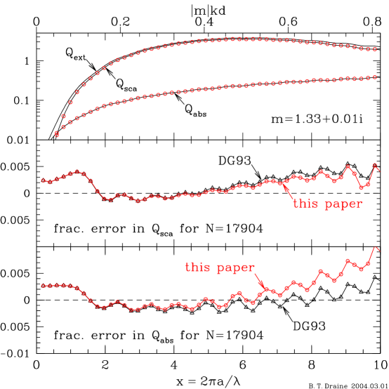
Figure 1: DDA calculations of scattering and absorption by a sphere with refractive index $m=1.33+0.01i$. Upper panel shows $Q_{\rm sca}$, $Q_{\rm abs}$, and $Q_{\rm ext}\equiv Q_{\rm sca}+Q_{\rm abs}$ calculated using Mie theory (solid curves) and using the DDA with $N=17904$ and the present polarizabilities. Middle and lower panels show fractional errors for $Q_{\rm sca}$ and $Q_{\rm abs}$. Circles: using dipole polarizabilities from this paper (eq.(69). Triangles: using dipole polarizabilities from Draine & Goodman (1993);

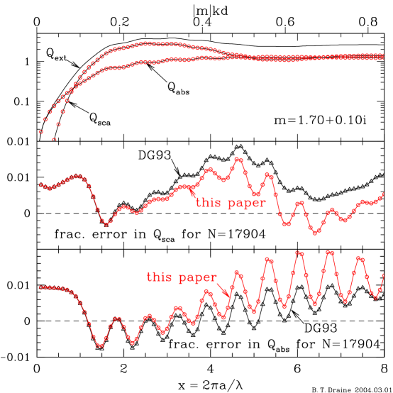
Figure 2: As in Figure 1, but for $m=1.7+0.1i$.

4 DDA Scattering Tests

We now compare discrete dipole approximation (DDA) calculations of scattering and absorption using (1) the polarizability prescription (67) from DG93 and (2) the present result (69). We consider spheres where we can use Mie theory to easily calculate the exact result for comparison. Let $C_{\rm sca}$ and $C_{\rm abs}$ be the cross sections for scattering and absorption, and let $Q_{\rm sca}\equiv C_{\rm sca}/\pi a^{2}$ and $Q_{\rm abs}\equiv C_{\rm abs}/\pi a^{2}$ be the dimensionless scattering and absorption efficiency factors for a sphere of radius $a$.

Figure 1 shows $Q_{\rm sca}$ and $Q_{\rm abs}$ calculated using the DDA with a target consisting of $N=17904$ dipoles, with radius $a=a_{\rm eff}\equiv(3N/4\pi)^{1/3}d$. The DDA calculations used a cubic lattice, and were carried out using the public domain code DDSCAT.6.1 (Draine & Flatau, 2004). Calculations were done for values of the scattering parameters $x\equiv 2\pi a/\lambda$ satisfying $|m|kd<0.8$, as this appears to be a good validity criterion for DDA calculations. The upper panel shows scattering and absorption efficiencies calculated with Mie theory and using the DDA with the present prescription for polarizabilities ff. The middle and lower panels show fractional errors $[Q({\rm DDA})/Q({\rm Mie})-1]$ of the DDA scattering and absorption cross sections.

Because the DDA target (dipoles on a cubic lattice) is not rotationally symmetric, the scattering problem was solved for 12 different incident directions, in each case for two orthogonal polarizations. The cross sections shown in Fig. 1 are averages over the 12 incident directions and two incident polarizations.

In the limit $x\rightarrow 0$, identical results are obtained for both polarizability prescriptions; this is expected since they differ only in terms of $O(|m|^{2}(kd)^{2})$. Note that even at $x=0$ (i.e., $kd=0$) – for which the polarizabilities are exactly given by the Clausius-Mossotti polarizabilities – the DDA calculation has a nonzero error even as $x\rightarrow 0$ and $kd\rightarrow 0$. This is because (1) the dipole array only approximates a spherical geometry and (2) when the “lattice dispersion relation” polarizabilities are used, the DDA does not accurately model the “screening” of the target material close to the surface by the polarization at the target surface. For modest dielectric functions, and sufficient numbers of dipoles, the errors are small – for the case shown in Figure 1 the fractional errors in the $x\rightarrow 0$ limit are $<0.3\%$.

As $x$ increases, the two prescriptions result in differences in computed values of $Q_{\rm sca}$ and $Q_{\rm abs}$, although the differences are small, and comparable in magnitude to the errors in the $x\rightarrow 0$ limit. In Figure 1 our new prescription appears to result in small improvements in accuracy (relative to DG93) for $Q_{\rm sca}$ for $|m|kd<0.8$, and likewise for $Q_{\rm abs}$ for $|m|kd<0.5$. For $0.5<|m|kd<0.8$, however, the DG93 prescription appears to give more accurate results for $Q_{\rm abs}$. Note, however, that for both polarizability prescriptions the fractional errors in $Q_{\rm sca}$ and $Q_{\rm abs}$ for $|m|kd\approx 0.5$ are of the same order as the fractional errors for $kd\rightarrow 0$, so it is not clear that the errors should be attributed to the lattice dispersion relation – the errors in $Q_{\rm sca}$ and $Q_{\rm abs}$ may instead be associated with errors in the computed polarization field near the surfaces, arising from the fact that in the DDA the dipoles in the surface layer are imperfectly “screened” from the external field by their neighbors.

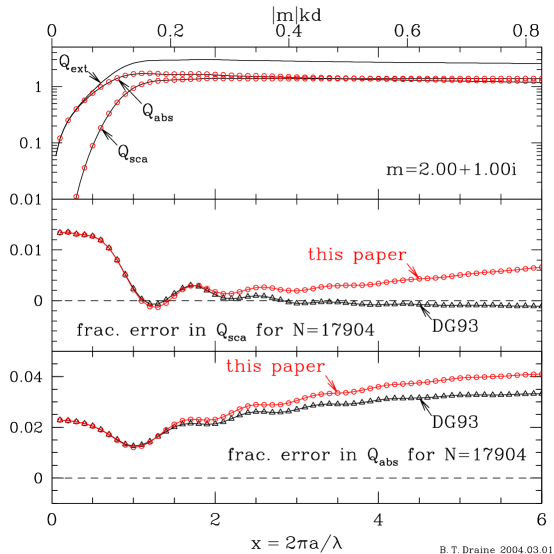
Figure 3: As in Figure 1, but for $m=2+i$.

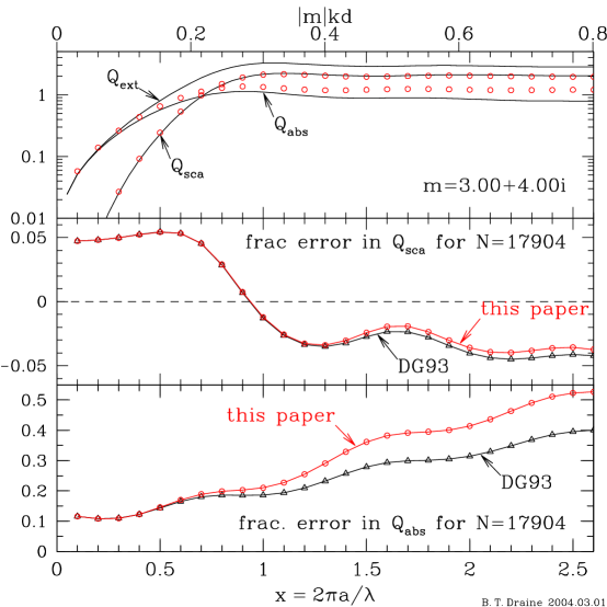
Figure 4: As in Figure 1, but for $m=3+4i$.

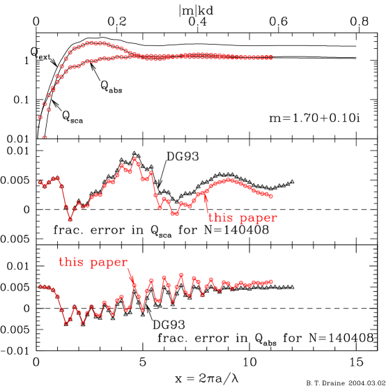
Figure 5: As in Figure 2, but for $N=140408$ dipoles.

For $|m|kd<0.8$, the errors in $Q_{\rm sca}$ using the new polarizabilities are of order $\sim 1\%$ for $m=1.33+0.01i$ (Figure 1), $m=1.7+0.1i$ (Figure 2) and $m=2+i$ (Figure 3), and of order $\sim 5\%$ for $m=3+4i$ (Figure 4). In all four cases, for wavelengths satisfying $|m|kd<0.8$, the magnitude of the error in $Q_{\rm sca}$ is of the same order as the error at zero frequency, suggesting that it is mainly due to the surface.

The errors in $Q_{\rm abs}$ tend to be somewhat larger than for $Q_{\rm sca}$, especially for large values of ${\rm Im}(m)$. For $m=3+4i$ (Figure 4), the new polarizabilities result in a fractional error of $\sim 50\%$ for $x=2.6$ and $N=17904$ dipoles.

Figure 5 shows results calculated for $m=1.7+0.1i$ spheres represented by $N=140408$ dipoles – 8 times as many as in Fig. LABEL:fig:m=1.70_0.10i. Note that the fractional error for $x\rightarrow 0$ is now only 0.5% – half as large as for $N=17904$. This can be ascribed to the fact that the fraction of the dipoles in the surface monolayer was reduced by a factor of 2. Note also that the errors for finite $x$ are also about a factor of 2 smaller than for $N=17904$. These results appear to confirm the suspicion that the errors arise primarily from the surface layer.

Rahmani et al. (2002) recently proposed a method for assigning dipole polarizabilities that takes into account the effects of target geometry, resulting in dipole polarizabilties that are location-dependent even when the target being approximated has homogeneous composition. Collinge & Draine (2004) have extended this treatment by adding finite-wavelength corrections to the “surface-corrected” polarizability prescription, and used DDA calculations for spheres and ellipsoids to show that accurate results for $Q_{\rm sca}$ and $Q_{\rm abs}$ can be obtained for modest numbers of dipoles even when the target material has a large refractive index $|m|\geq 5$. The current calculations does not include such “surface corrections”, – the prescription (69) depends only on local properties – so it comes as no surprise that there are systematic errors even in the limit $x\rightarrow 0$.

Collinge & Draine (2004) show that the error can be greatly reduced if the polarizabililites are assigned in a way that allows for both target geometry (i.e., surface corrections) and the finite wavelength corrections obtained from the lattice dispersion relation analysis. Using these “surface-corrected lattice dispersion relation polarizabilities”, Collinge & Draine (2004) show that for the case $m=3+4i$, the error in $Q_{\rm abs}$ can be reduced to of order $1\%$ for $x=0.83$ using as few as $N=5904$ dipoles, whereas for $x=0.83$, the error is seen from Figure 4 to be $\sim 20\%$ even with $N=17904$ dipoles. Such surface corrections will obviously be of value for DDA calculations, but at the moment have been applied only to sperical, spheroidal, or ellipsoidal targets (Collinge & Draine, 2004).

5 Summary

The principal results of this paper are as follows:

1. We have derived the exact mode equation (31) for propagation of electromagnetic waves through a rectangular lattice of polarizable points.

2. If the electric polarizability tensor $\alpha$ for the lattice points is specified, then we can solve the mode equation to obtain the dispersion relation for waves propagating on the lattice. Alternatively, if we wish the lattice to have the same dispersion relation as a continuum medium of complex refractive index $m$, then we can solve the mode equation for the appropriate polarizability tensor.

3. In the case of a cubic lattice, our derived “lattice dispersion relation” polarizability tensor (69) is diagonal but anisotropic, and differs from the isotropic polarizabilities obtained by DG93.

4. The new polarizability prescription has been tested in DDA scattering calculations for spheres. The resulting cross sections have accuracies comparable to those obtained with the DG93 prescription.

Appendix A Numerical Results for $R_{0}(i)$, $R_{1}$, $R_{2}(i)$, and $R_{3}(i,j)$

The coefficients $R_{0}(i)$ are obtained numerically from the sums (45). Note that eq. (45) for $R_{0}$ involves the difference between two sums which separately diverge at infinity. To handle this divergence, one notes that in nature one is always interested in finite wavelengths and nonzero frequencies; when dealing with finite wavelengths, the lattice sums converge because of the oscillations introduced at large distances by retardation effects. To obtain the proper behavior when going to the zero frequency limit, we modify the summations to suppress the contribution from large distances. The manner in which this is achieved is not critical. We compute

$$R_{0}(i)=\lim_{\alpha\rightarrow 0}\left[\sum_{\bf n}{n_{i}^{2}\over|{\bf n}|^{2}}\exp(-\alpha|{\bf n}|^{4})-\sum_{\bf n}{Q_{i}^{2}\over|{\bf Q}|^{2}}\exp(-\alpha|{\bf Q}|^{4})\right]$$ (A1)

The exponential cutoff allows one to limit the summations to $\alpha|{\bf n}|^{4}<20$ and $\alpha|{\bf Q}|^{4}<20$. The summation (A1) is carried out for various small values of $\alpha$ and it is found, as anticipated, that for $\alpha<10^{-8}$ the numerical result for $R_{0}$ is insensitive to the choice of $\alpha$. Each of the sums in (A1) is over a lattice; $|{\bf n}|^{2}$ defines the distance from the origin for the cubic lattice, and $|{\bf Q}|^{2}$ is the distance from the origin for the reciprocal lattice. Each sum diverges at infinity, where we can replace the discrete summation by an integration; the reason why the divergences cancel is that the two lattices have the same density of lattice points, so that at large distances, both approach the same integration.

Table 1: $R_{0}(i)$ for selected values of $d_{1}:d_{2}:d_{3}$

$d_{1}$	$d_{2}$	$d_{3}$	$R_{0}(1)$	$R_{0}(2)$	$R_{0}(3)$
1	1	1	0	0	0
1	1	1.5	0.20426	0.20426	-0.40851
1	1.5	1.5	0.52383	-0.26192	-0.26192
1	1	2	0.38545	0.38545	-0.77090
1	1.5	2	0.81199	-0.21028	-0.60172
1	2	2	1.19693	-0.59846	-0.59846
1	1	3	0.74498	0.74498	-1.48995
1	1.5	3	1.38481	-0.14304	-1.24176
1	2	3	1.96224	-0.69714	-1.26510
1	3	3	3.11030	-1.55515	-1.55515

The quantities $R_{1}$, $R_{2}$, and $R_{3}$ appearing in the dispersion relation in the limit of small but nonzero frequency $\nu$ have been obtained by direct evaluation of $R_{3}(i,j)$ using eq. (49) followed by use of equations (50) and (51) to obtain $R_{1}$ and $R_{2}(i)$. Six elements of the symmetric matrix $R_{3}(i,j)$ are given in Table 2.

Finally, $R_{1}$ and $R_{2}(i)$ are given in Table 3.

Table 2: $R_{3}(i,j)$ for selected values of $d_{1}:d_{2}:d_{3}$

$d_{1}$	$d_{2}$	$d_{3}$	$R_{3}(1,1)$	$R_{3}(2,2)$	$R_{3}(3,3)$	$R_{3}(1,2)$	$R_{3}(1,3)$	$R_{3}(2,3)$
1	1	1	0.00000	0.00000	0.00000	0.00000	0.00000	0.00000
1	1	1.5	0.37743	0.37743	-1.62922	0.13566	0.01609	0.01609
1	1.5	1.5	0.80161	-0.80815	-0.80815	0.16648	0.16648	-0.18041
1	1	2	0.55693	0.55693	-3.72878	0.23735	0.09360	0.09360
1	1.5	2	1.02166	-0.55501	-2.30887	0.27206	0.25987	-0.21806
1	2	2	1.26456	-1.78732	-1.78732	0.37528	0.37528	-0.39535
1	1	3	0.81662	0.81662	-8.83412	0.39793	0.23223	0.23223
1	1.5	3	1.34832	-0.40088	-6.06792	0.43771	0.42272	-0.15845
1	2	3	1.62638	-1.56624	-4.80661	0.55590	0.55480	-0.48211
1	3	3	2.04073	-3.94766	-3.94766	0.76142	0.76142	-0.90991

Table 3: $R_{1}$ and $R_{2}(i)$ for selected values of $d_{1}:d_{2}:d_{3}$

$d_{1}$	$d_{2}$	$d_{3}$	$R_{1}$	$R_{2}(1)$	$R_{2}(2)$	$R_{2}(3)$
1	1	1	0.00000	0.00000	0.00000	0.00000
1	1	1.5	-0.53869	0.52918	0.52918	-1.59705
1	1.5	1.5	-0.50962	1.13457	-0.82209	-0.82209
1	1	2	-1.76582	0.88788	0.88788	-3.54158
1	1.5	2	-1.21448	1.55359	-0.50100	-2.26706
1	2	2	-1.59967	2.01512	-1.80739	-1.80739
1	1	3	-5.47612	1.44677	1.44677	-8.36967
1	1.5	3	-3.71651	2.20875	-0.12162	-5.80365
1	2	3	-3.48931	2.73708	-1.49246	-4.73393
1	3	3	-4.62875	3.56356	-4.09616	-4.09616

References

- Ashcroft & Mermin (1976) Ashcroft, N.W, & Mermin, N.D. 1976, Solid State Physics (New York: Holt, Rinehart, & Winston)
- Collinge & Draine (2004) Collinge, M.J., & Draine, B.T. 2004, “Discrete-dipole approximation with polarizabilities that account for both finite wavelength and target geometry”, J. Opt. Soc. Am., A, submitted (http://xxx.arxiv.org/abs/astro-ph/0311304v1)
- Draine (1988) Draine, B.T. 1988, “The Discrete-Dipole Approximation and its Application to Interstellar Graphite Grains”, Astrophys. J., 333, 848
- Draine & Flatau (1994) Draine, B.T., & Flatau, P.J. 1994, “Discrete dipole approximation for scattering calculations”, J. Opt. Soc. Am., A, 11, 1491
- Draine & Flatau (2004) Draine, B.T., & Flatau, P.J. 2004, “User Guide for the Discrete Dipole Approximation Code DDSCAT.6.1”, http://arxiv.org/abs/astro-ph/xxx
- Draine & Goodman (1993) Draine, B.T., & Goodman, J. 1993, “Beyond Clausius-Mossotti: Wave Propagation on a Polarizable Point Lattice and the Discrete Dipole Approximation”, Astrophys. J., 405, 685 (DG93)
- Draine & Weingartner (1996) Draine, B.T., & Weingartner, J.C. 1996, “Radiative Torques on Interstellar Grains: I. Superthermal Rotation”, Astrophys. J., 470, 551
- Draine & Weingartner (1997) Draine, B.T., & Weingartner, J.C. 1997, “Radiative Torques on Interstellar Grains: II. Alignment with the Magnetic Field”, Astrophys. J., 480, 633
- Goodman, Draine & Flatau (1991) Goodman, J.J., Draine, B.T., & Flatau, P.J. 1991, “Application of FFT Techniques to the Discrete Dipole Approximation”, Optics Letters, 16, 1198
- Jackson (1962) Jackson, J.D. 1962, Classical Electrodynamics, (New York: Wiley)
- Rahmani et al. (2002) Rahmani, A., Chaumet, P.C., & Bryant, G.W. 2002, “Coupled dipole method with an exact long-wavelength limit and improved accuray at finite frequencies”, Opt. Lett., 27, 2118