The Internal Structural Adjustment due to Tidal Heating of Short-Period Inflated Giant Planets

Abstract

Several short-period Jupiter-mass planets have been discovered around nearby solar-type stars. During the circularization of their orbits, the dissipation of tidal disturbance by their host stars heats the interior and inflates the sizes of these planets. Based on a series of internal structure calculations for giant planets, we examine the physical processes which determine their luminosity-radius relation. In the gaseous envelope of these planets, efficient convection enforces a nearly adiabatic stratification. During their gravitational contraction, the planets’ radii are determined, through the condition of a quasi-hydrostatic equilibrium, by their central pressure. In interiors of mature, compact, distant planets, such as Jupiter, degeneracy pressure and the non-ideal equation of state determine their structure. But, in order for young or intensely heated gas giant planets to attain quasi-hydrostatic equilibria, with sizes comparable to or larger than two Jupiter radii, their interiors must have sufficiently high temperature and low density such that degeneracy effects are relatively weak. Consequently, the effective polytropic index monotonically increases whereas the central temperature increases and then decreases with the planets’ size. These effects, along with a temperature-sensitive opacity for the radiative surface layers of giant planets, cause the power index of the luminosity’s dependence on radius to decrease with increasing radius. For planets larger than twice Jupiter’s radius, this index is sufficiently small that they become unstable to tidal inflation. We make comparisons between cases of uniform heating and cases in which the heating is concentrated in various locations within the giant planet. Based on these results we suggest that accurate measurement of the sizes of close-in young Jupiters can be used to probe their internal structure under the influence of tidal heating.

1 Introduction

One of the surprising findings in the search for planetary systems around other stars is the discovery of extrasolar planets with periods down to 3 days (Mayor & Queloz (1995)). Nearly all planets with period less than 7 days have nearly circular orbits. In contrast, known extrasolar planets with periods longer than 2-3 weeks, have nearly a uniform eccentricity distribution. The shortest-period planets and their host stars induce tidal perturbations on each other. When these disturbances are dissipated, angular momentum is exchanged between the planets and their host stars, leading toward both a spin synchronization and orbital circularization (Rasio et al. (1996)).

Bodenheimer, Lin, & Mardling (2001) (hereafter Paper I), considered the effect of tidal dissipation of energy during the synchronization of these planets’ spin and the circularization of their orbits. In that analysis, they compute a series of numerical models for the interior structures of weakly eccentric Jovian planets at constant orbital distances under the influence of interior tidal heating and stellar irradiation. In these previous calculations, the interior heating rate per unit mass was imposed to be constant in time and uniformly distributed within the planet. Under these assumptions, they showed that Jovian planets can be inflated to equilibrium sizes considerably larger than those deduced for gravitationally contracting and externally heated planets. For the transiting planet around HD 209458, they suggested that provided its dimensionless dissipation $Q$-value is comparable to that inferred for Jupiter (Yoder & Peale (1981)), a small eccentricity ($e\simeq 0.03$) would provide adequate tidal heating to inflate it to its observed size (Brown et al. (2001)). Since the orbital circulation time scale is expected to be shorter than the life span of the planet, they also suggested that this eccentricity may be excited by another planet with a longer orbital period. The prediction of a small eccentricity and the existence of another planet are consistent with existing data (Bodenheimer, Laughlin, & Lin (2003)).

There are at least two other scenarios for the unexpectedly large size of HD 209458b. Heating by stellar irradiation reduces the temperature gradient and the radiative flux in the outer layers of short-period planets. This process could significantly slow down the Kelvin-Helmholtz contraction of the planet and explain the large size (Burrows et al. (2000)). However, even though the stellar flux onto the planet’s surface is 5 orders of magnitude larger than that released by the gravitational contraction and cooling of its envelope, this heating effect alone increases the radius of the planet by about 10%, not by 40% as observed (Guillot & Showman (2002)).

An alternative source is the kinetic heating induced by the dissipation of the gas flow in the atmosphere which occurs because of the pressure gradient between the day and night sides (Guillot & Showman (2002)). In order to account for the observed size of the planet, conversion of only 1% of the incident radiative flux may be needed, provided that the dissipation of induced kinetic energy into heat occurs at sufficiently deep layers (tens to 100 bars). Showman & Guillot (2002) suggest that the Coriolis force associated with a synchronously spinning planet may induce the circulation to penetrate that far into the planet’s interior, and that dissipation could occur through, for example, Kelvin-Helmholtz instability. A follow-up analysis suggests that this effect may be limited (Burkert et al. (2003); Jones & Lin (2003)).

In order to distinguish between these three scenarios, the effect of tidal heating for planets with modest to large eccentricities was considered. In a follow-up paper (Gu et al. 2003, hereafter Paper II), we showed that the size ($R_{p}$) of compact Jupiter-mass planets slowly increases with the tidal dissipation rate. For computational simplicity, we adopted a conventional equilibrium tidal model which describes the planets’ continuous structural adjustment in order for them to maintain a state of quasi-hydrostatic equilibrium in the varying gravitational potential of their orbital companion. In this prescription, a phase lag into the response is introduced to represent the lag being proportional to the tidal forcing frequency and attributable to the viscosity of the body. The phase lag gives rise to a net tidal torque and dissipation of energy and the efficiency of the tidal dissipation can be parametrized, whatever its origin, by a specific dissipation function or $Q$-value (quality factor) (Goldreich & Soter (1966)). External perturbation can also induce dynamical tidal responses through the excitation of g modes (Ioannou & Lindzen 1993a,b) or inertial waves (Ogilvie & Lin (2004)) which can be damped by viscous dissipation in the interior (Goldreich & Nicholson (1977)) or radiative and nonlinear dissipation in the atmosphere of the planet (Lubow et al. (1997)).

In both the prescription for equilibrium and dynamical responses, the tidal dissipation rate is a rapidly increasing function of the planets’ radius. But, their surface luminosity increases even faster with $R_{p}$ such that, planets with relatively small eccentricities and modest to long periods attain a state of thermal equilibrium in which the radiative loss on their surface is balanced by the tidal dissipation in their interior. For planets with short periods and modest to large eccentricities, the rate of interior heating is sufficiently large that their $R_{p}$ may inflate to more than two Jupiter radii. In this limit, the surface luminosity of the planet becomes a less sensitive function of its $R_{p}$ and the eccentricity damping rate is smaller than the expansion rate of the planet so that the increases in their surface cooling rate cannot keep pace with the enhanced dissipation rate due to their inflated sizes. These planets are expected to undergo runaway inflation and mass loss. We suggested that the absence of ultra-short-period Jupiter-mass planets with $P<3$ days, which corresponds to an orbital semi-major axis $a$ of 0.04 AU, may be due to mass loss through Roche-lobe overflow resulting from such a tidal inflation instability. Other scenarios have been proposed to explain the lack of Jupiter-mass planets with $P<3$ days: truncation of inner part of a disk (Lin et al. (1996); Kuchner & Lecar (2002)), orbital migration due to the spin-orbit tidal interaction between the close-in planet and the parent star (Rasio et al. (1996); Witte & Savonije (2002); Paetzold & Rauer (2002); Jiang et al. (2003)), and Roche-overflowing planets with the help of disk-planet interaction but without tidal inflation (Trilling et al. (1998)).

In this contribution, we continue our investigation on the internal structure of tidally heated short-period planets. The main issues to be examined here are: 1) how does tidal energy dissipation actually lead to the expansion of the envelope? 2) how does the internal structure of the planet depend on the distribution of their internal tidal dissipation rate? and 3) what are the important physical effects which determine the tidal inflation stability of the planets? These issues are important in determining the mass-radius relation of short-period planets which is directly observable.

Structural adjustments may also modify the efficiency of dissipation and the planets’ Q-value for both equilibrium and dynamical tides. In the extended convective envelopes of gaseous giant planets and low-mass stars, turbulence can lead to dissipation of the motion that results from the continual adjustment of the equilibrium tide. However, the turbulent viscosity estimated from the mixing-length theory ought to be reduced by a frequency-dependent factor owing to the fact that the convective turnover time scale is usually much longer than the period of the tidal forcing. Based on the present-day structure of Jupiter, Goldreich & Nicholson (1977) estimated $Q\approx 5\times 10^{13}$. However, within the intensely heated (by tidal dissipation) short-period extra solar planets, convection is expected to be more rigorous with higher frequencies whereas their tidal forcing frequencies are smaller than that of Jupiter. The Q-value for the equilibrium tide within extra solar planets is likely to much smaller than that within Jupiter.

For the dynamical response of short-period extra solar planets planet, the forcing frequencies are typically comparable to their spin frequencies but are small compared to their dynamical frequencies. Convective regions of the planets support inertial waves, which possess a dense or continuous frequency spectrum in the absence of viscosity, while any radiative regions support generalized Hough waves (Ioannou & Lindzen 1993a, b). Inertial waves provide a natural avenue for efficient tidal dissipation in most cases of interest. The resulting value of $Q$ depends, in principle, in a highly erratic way on the forcing frequency. Since the planets’ spin frequency adjusts with their $R_{p}$, which is a time-delayed function of the tidal dissipation rate within them, the efficiency of tidal dissipation may fluctuate while the overall evolution is determined by a frequency-average Q-value (Ogilvie & Lin (2004)).

In §2, we briefly recapitulate the basic equations which determine the quasi-static evolution of the planets’ structure. We show the simulation results for inflated giant planets in the case of constant internal heating per unit mass in §3 and analyze the results, in the Appendix, in terms of polytropic models which allow us to conclude that the onset of the tidal runaway inflation instability is regulated by a transition in the equation of state for the interior gas from a partially degenerate/non-ideal state toward a more ideal-gas state. We examine the dependence of planetary adjustment on different locations of the energy dissipation in §4. Finally, we summarize the results and discuss their observational implications in §5.

2 The Planetary Structure Equations and Numerical Methods

The internal structure of an inflated Jupiter is constructed in this paper with the same numerical scheme as that used in Paper I. The code employs the tabulated equation of state and adiabatic gradient $\nabla_{\rm ad}$ described by Saumon, Chabrier, & Van Horn (1995) and the values of opacities are derived from those provided by Alexander & Ferguson (1994). With this scheme, we compute distributions of thermodynamical parameters as a function of radius for a spherically symmetric planet (i.e. 1-D calculation). The surface temperature of the planet is assumed to be maintained by the irradiation from a solar-type star located 0.04 AU away. The structure of the planet is assumed to be hydrostatic and not to be affected by rotation since the nearly synchronized short-period planets spin at least several times slower than Jupiter and their rotational energy is quite small compared to their gravitational energy (paper I)

The models include a tidal heating function, whose physical basis is not well understood. Thus in §3 we consider simulations in which the planet has a constant internal heating which is uniform in mass. In §4 we consider a set of models in which the heating is non-uniform in mass. As discussed by Ogilvie & Lin (2004), different mechanisms may operate in radiative or convective layers. One should, in principle allow for three avenues of tidal dissipation: viscous dissipation of the equilibrium tide, viscous dissipation of inertial waves, and emission of Hough waves in the radiative zone. Rotational effects can also affect the behavior of tidal dissipation. In view of the uncertainties, we do not model specific mechanisms but simply parameterize the heating rate.

In our calculations, we assume that convection is so efficient that the temperature gradient behaves adiabatically within a convective zone (Guillot et al. 2003). In other words, we solve the following equations for the radius $r$, the density $\rho$, the pressure $P$, the temperature $T$, and the intrinsic luminosity $\cal L$ (e.g. see Kippenhahn & Weigert (1990))

$${\partial r\over\partial m} = {1\over 4\pi r^{2}\rho},$$ (1)

$${\partial P\over\partial m} = -{Gm\over 4\pi r^{4}},$$ (2)

$${\partial T\over\partial m} = -{GmT\over 4\pi r^{4}P}\nabla,$$ (3)

$$\nabla = \nabla_{rad}={3\over 16\pi acG}{\kappa{\cal L}P\over mT^{4}}\ \ {\rm if\ radiative};\qquad\nabla=\nabla_{\rm ad}\ \ {\rm if\ convective},$$ (4)

$${\partial{\cal L}\over\partial m} = \epsilon-c_{P}{\partial T\over\partial t}+{\delta\over\rho}{\partial P\over\partial t},$$ (5)

where $m$ is the Lagrangian mass coordinate, $\delta$ ($\equiv-(\partial\ln\rho/\partial\ln T)_{P}$) is the coefficient of thermal expansion at constant pressure, $c_{P}$ is the specific heat at constant pressure, $\epsilon$ is the heating rate per unit mass, and $\nabla$ is defined as $d\ln T/d\ln P$.

The above structure equations are solved simultaneously with an 1-D implicit Lagrangian scheme which uses the mass coordinate $m$ as an independent variable. In the case where the heating rate is uniformly distributed with mass (i.e. $\epsilon=$constant), the results of our numerical calculations usually show that the planet interior is largely convective. Consequently, without the aid of the energy equation (5), equations (1) –(4) imply that the adiabatic assumption gives rise to a unique radial stratification for a given planet’s size and mass, regardless of how strong the internal heating rate is or whether the planet is in thermal equilibrium. Equation (5) then indicates how fast the planet expands or contracts due to thermal imbalance. These adjustments proceed through a series of quasi-hydrostatic and quasi-thermal equilibria.

The initial condition is obtained from calculations for the formation phases of planets of the appropriate masses, as described in Bodenheimer et al. (2000). Just after accretion ends, those calculations show that the radius is about $2R_{J}$, which is the initial condition used here. This value is somewhat uncertain, and it changes quite rapidly during the earliest part of the planet’s cooling phase, but the exact value makes little difference here, because most of the models reach a thermal equilibrium which is practically independent of the initial state.

For the inner boundary, we consider models with or without cores. For the models with cores, we assume that they have a constant density $\rho_{\rm core}=5$ g cm^-3. Their temperature is also assumed to be the same as that of the envelope immediately outside the core. The luminosity generated in the cores is assumed to be negligible. In most of our models, the central temperature is above $\sim 3\times 10^{4}$ K, and the heavy elements in the cores are likely to be soluble (Paper I). Since we have already shown that core-less models lead to more inflated planetary structure, the planetary radii determined for the core models represent a lower limit. There are some uncertainties in the equation of state at the temperatures and pressures of the central regions, where the hydrogen-helium gas is partially degenerate and non-ideal. We show below that the degree of degeneracy and the non-ideal effects are important in determining the stability against the tidal runaway instability.

Near the planet’s surface, the gas becomes radiative when $\nabla_{r}<\nabla_{ad}$, where $\nabla_{r}$ is computed using equation (4) and $\nabla_{ad}$ is obtained from a tabulated equation of state. The depth of the radiative zone is sensitive to the opacity. The temperature of the surface layer is sufficiently low for grains to condense. We adopt the standard opacity table (Alexander & Ferguson (1994)) which is computed for the interstellar gas. However, in Jupiter’s atmosphere the sedimentation of grains leads to a much reduced opacity which modifies the structure of the radiative zone. For short-period planets, however, the side facing the host star is heated to $\sim 1,500$ K which is near or above the sublimation temperature of most grain species. In addition, a large scale circulation flow may also modify the composition and the heat transport process near the surface. It remains to be determined whether grain sedimentation occurs (Burkert et al. 2003). In order to take into account this possibility, we consider some models under the assumption of extreme grain depletion, i.e. without any grain opacity, so that the effective opacity $\kappa_{d}$ is reduced from the normal opacity $\kappa_{0}$ (see Table 2).

At the surface of the planet, we include the irradiation from the star in the boundary condition for the temperature $T_{surf}$. We neglect the difference between the day and night sides of the planet. For most of the models, we set the irradiation temperature $T_{0}=1500$ K, which corresponds to a planet with a 3-day period around a solar-type star. For two models, we also considered somewhat lower temperatures. At the photosphere, the normal boundary conditions for pressure $P=2GM_{p}/3\kappa_{d}R_{p}^{2}$ and for the intrinsic luminosity ${\cal L}=4\pi\sigma R_{p}^{2}(T_{surf}^{4}-T_{0}^{4})$ are adopted.

3 Constant internal heating per unit mass

In this section, we shall show the numerical results for an internal heating rate that is constant in time and is uniform in mass; that is, $\epsilon$ in equation (5) takes a constant value. The calculations are carried out for three different masses: $0.63M_{J}$, $1M_{J}$, and $3M_{J}$. The time span for each calculation covers a few $10^{9}$ years. At the end of each computation, the planets have attained a thermal equilibrium. In this state, the integrated energy term $\epsilon$ in equation (5) balances the intrinsic radiated luminosity. Normally when a planet contracts and cools, the time-dependent terms in equation (5) dominate, and a thermal balance is never reached. The same is true even if the planet is strongly irradiated by the star. However the present results show that an internal tidal energy dissipation rate on the order of $10^{27}$ to $10^{30}$ erg per second, depending on the mass, is sufficient to stop the contraction and cooling at some radius in the range of a few $R_{J}$.

In Figure 1, we show that there exists a radius-luminosity relation for a Jovian planet with a given mass $M_{p}$. The planet’s intrinsic luminosity (i.e. excluding the luminosity due to stellar irradiation) emitted from the photosphere is denoted by $\cal L$. Discrete points shown in the Figure are our computational results, which are fitted by three quadratic curves associated with three different masses. For a $0.63M_{J}$ core-less planet, the solid curve in the left panel can be approximated by,

$$\log({\cal L}/10^{27}{\rm erg/s})=-11.7039(\log(R_{p}/R_{J}))^{2}+12.8994\log(R_{p}/R_{J})-2.12471.$$ (6)

For the same mass planet with a core (solid curve in the right panel), we can approximate

$$\log({\cal L}/10^{27}{\rm erg/s})=-8.78501(\log(R_{p}/R_{J}))^{2}+10.004\log(R_{p}/R_{J})-1.05358.$$ (7)

Similarly, the model without a core (dashed curve in the left panel) and with a core (dashed curve in the right panel) for a $1M_{J}$ planet can be approximated by

$$\log({\cal L}/10^{27}{\rm erg/s})=-7.7909(\log(R_{p}/R_{J}))^{2}+10.3338\log(R_{p}/R_{J})-1.20809,$$ (8)

$$\log({\cal L}/10^{27}{\rm erg/s})=-6.74289(\log(R_{p}/R_{J}))^{2}+8.92021\log(R_{p}/R_{J})-0.573055$$ (9)

respectively. Finally, $3M_{J}$ models without a core (dotted curve in the left panel) and with a core (dotted curve in the right panel) can be approximated by

$$\log({\cal L}/10^{27}{\rm erg/s})=-8.10772(\log(R_{p}/R_{J}))^{2}+10.6893\log(R_{p}/R_{J})-0.29812,$$ (10)

$$\log({\cal L}/10^{27}{\rm erg/s})=-10.525(\log(R_{p}/R_{J}))^{2}+12.3851\log(R_{p}/R_{J})-0.508571$$ (11)

respectively.

For large values of $R_{p}$, these three curves all become flattened as the planet is inflated; i.e. as the planet expands, the slope ($\gamma\equiv d\log{\cal L}/d\log R_{p}$) decreases. In the core-less cases, $\gamma=5$ at $R_{p}=2.175R_{J}$ for $M_{p}=0.63M_{J}$, $R_{p}=2.199R_{J}$ for $M_{p}=1M_{J}$, and $R_{p}=2.243R_{J}$ for $M_{p}=3M_{J}$. In the core cases, $\gamma=5$ at $R_{p}=1.927R_{J}$ for $M_{p}=0.63M_{J}$, $R_{p}=1.953R_{J}$ for $M_{p}=1M_{J}$, and $R_{p}=2.243R_{J}$ for $M_{p}=3M_{J}$. Also, the luminosity for a given $R_{p}$ is an increasing function of $M_{p}$.

The results in Figure 1 do not correspond to the exact thermal equilibrium solutions. Although the planets quickly establish a hydrostatic equilibrium, ${\cal L}$ does not necessarily equal the internal heating rate. In these calculations, ${\cal L}$ is the instantaneous intrinsic luminosity associated with the corresponding $R_{p}$. We use various initial conditions for $R_{p}$ and $\epsilon$ for our computation, but the ${\cal L}$ vs $R_{p}$ curves remain nearly identical to those shown in Figure 1. This invariance is due to the adiabatic structure as we have stated in the previous section. The number marked on each data point is the degree of electron degeneracy at the center of the planet in the core-less cases or at the surface of the core in the core cases. The degree of electron degeneracy is expressed by the ratio of the Fermi energy to the thermal energy

$$D\equiv E_{Fermi}/kT\approx\rho/(6\times 10^{-9}T^{3/2}).$$ (12)

As shown in the figure, the degeneracy is lifted as the planet expands.

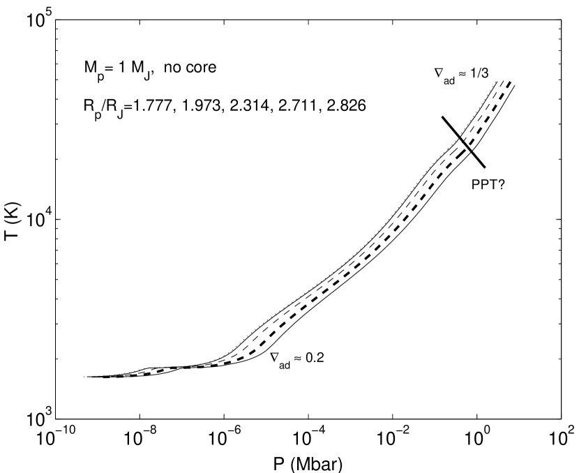
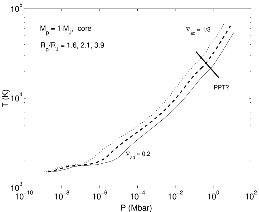
Figure 2: The temperature profiles against the pressure inside a planet of $1M_{J}$ with (right panel) and without (left panel) a core. Different curves are plotted for different $R_{p}$: The interior structure evolves from the lowest curve to the upper-most one as the planet expands.

In Figure 2, we plot the temperature against the pressure inside a planet with $M_{p}=1M_{J}$. Each curve corresponds to a different value of $R_{p}$. While the upper-right parts of the curves, where $T$ and $P$ are higher, represent the conditions for planet interiors, the lower-left portions of the curves show the $T$ and $P$ distribution near the planet’s surface. The thick line across the upper parts of the curves marks the “Plasma Phase Transition (PPT)” line which segregates hydrogen molecules and metallic hydrogen atoms. This line is approximately drawn based upon an extrapolation of a hydrogen phase diagram (Saumon et al. (1995)). As indicated by the slope of the curves, $\nabla_{ad}$ has a value $\simeq 1/3$ in the interiors where hydrogen atoms are in metallic form, and then drops down to around 0.2 as we follow the curves to the outer region of the planet where the pressure decreases below 10 bars. This transition occurs near the base of the radiative envelope. The flattening of $\nabla$ in the radiative envelope results from the external heating due to the stellar irradiation. The overall behavior of the curves for core and for core-less cases is very similar. In the core-less case, a decrease in the central pressure $P_{c}$ with the planet’s size can be fitted with a following power law

$$P_{c}\propto R_{p}^{-2.24}.$$ (13)

The above relation is less steep than what is expected from a purely polytropic structure in which $P_{c}\propto R_{p}^{-4}$. In addition, the central temperature $T_{c}$ increases with $R_{p}$ when $R_{p}\lesssim 2.3R_{J}$, but decreases with $R_{p}$ when $R_{p}\gtrsim 2.3R_{J}$. This variation of temperature is nearly independent of the strength of internal heating rates; that is, the variation of temperature profiles is almost the same for a given planet’s size no matter whether the planet is expanding, contracting or even in a thermal equilibrium. This tendency arises because, as stated in the previous section, adiabatic profiles are imposed in the convection zone which amounts to 95% of the total radius. The change of internal temperature in this manner is not driven by a thermal imbalance, but it is caused by an intrinsic change in the physical properties of the fluid in the convection zone as a result of the reduction of electron degeneracy (see Appendix A.2).

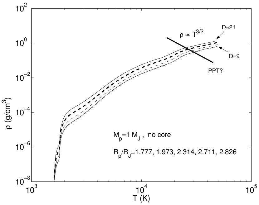
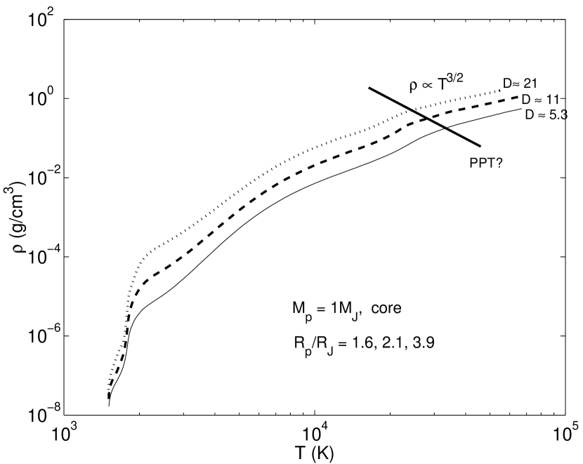
Figure 3: The mass density profiles as a function of the temperature for various planet’s sizes in the case of having a core (right panel) and having no core (left panel). The interior structure evolves from the upper-most curve to the lowest one as the planet expands.

Figure 3 displays the mass density profiles as a function of the temperature for various planet sizes. The theoretical Plasma Phase Transition line is also marked in the plot. Resembling the flattened $P-T$ curves in Figure 2, the steepening of the $T-\rho$ curves for $\rho$ less than about $10^{-4}$ g/cm³, which roughly corresponds to the region of radiative envelope, is caused by the stellar irradiation. We estimate the degree of degeneracy at the center of the planet with no core, and at the surface of the core for the planet with a core. As the planet with no core (with a core) expands from $1.777R_{J}$ to $2.826R_{J}$ ($1.6R_{J}$ to $3.9R_{J}$), the value $D$ declines from 21 to 9 (from 21 to 5.3) due primarily to the central density decrease. We fit the relation between $\rho_{c}$ and $R_{p}$ for the planet with no core by using the following power law

$$\rho_{c}\propto R_{p}^{-1.6}.$$ (14)

As is the case for the $R_{p}-P_{c}$ relation, which is described by equation (13), the power 1.6 in equation (14) is smaller than what is expected from a purely polytropic structure in which the power is 3.

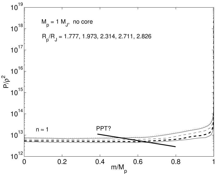
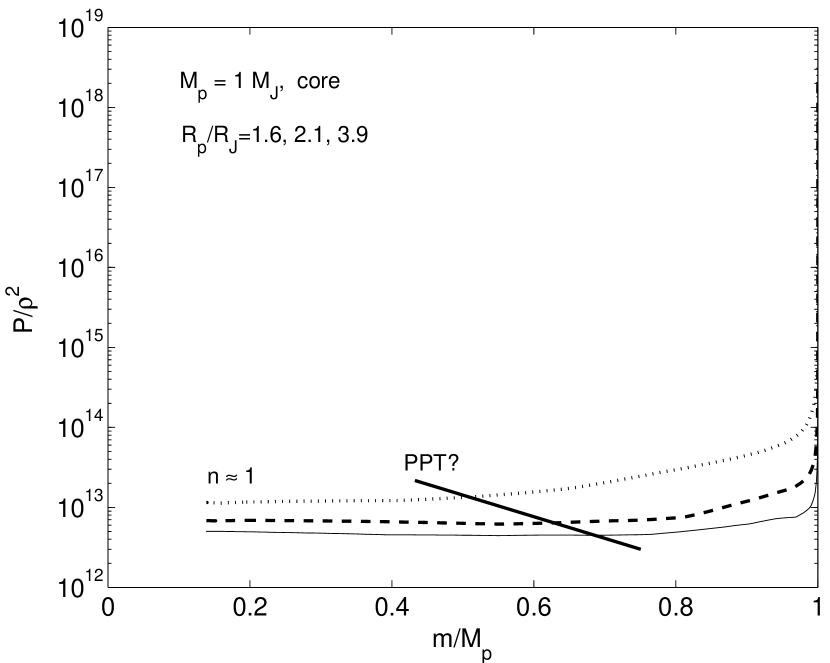
Figure 4: $P/\rho^{2}$ (in c.g.s units) as a function of the co-moving radial coordinate $m/M_{p}$ for various planet’s sizes in the cases of a planet with a core (right panel) and without a core (left panel). $m/M_{p}=0$ and $m/M_{p}=1$ represent the location of the planet’s center and the bottom of its photosphere respectively. The interior structure evolves from the lowest curve to the upper-most curve as the planet expands to different sizes indicated by $R_{p}/R_{J}$ shown at the upper-left corner of each panel.

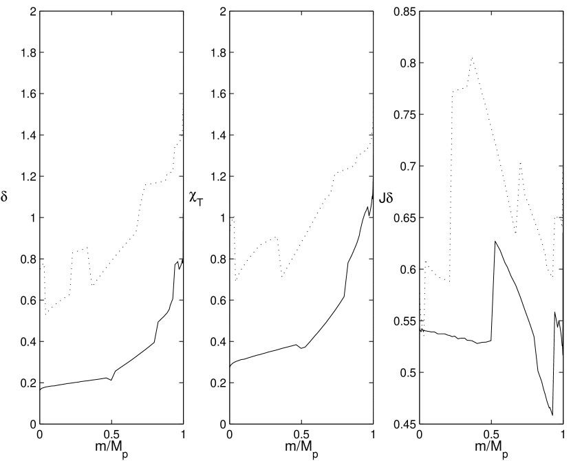
Figure 10: The coefficient of thermal expansion $\delta$, $\chi_{T}$, and $J\delta$ as a function of the co-moving mass coordinate $m/M_{p}$, plotted here for an inflated planet of $0.63M_{J}$ with two different radii: $1.66R_{J}$ (solid line) and $3.22R_{J}$ (dotted line).

The interior model of Jupiter is usually approximated by an $n=1$ polytrope, which results from the combination of Coulomb effects and electron degeneracy in the metallic hydrogen plasma (Hubbard (1984); Burrows et al. (2001)). This simplification is confirmed by the simulation as shown in Figure 4 which plots $P/\rho^{2}$ (in c.g.s units) as a function of the co-moving mass coordinate $m$ for various planet sizes. The hypothetical plasma phase transition line is denoted by PPT and is marked by a thick line. The almost constant value of $P/\rho^{2}$ throughout the region of metallic hydrogen indicates a $n\approx 1$ polytropic structure. As we follow these curves to the outer regions of the planet where the molecular hydrogen dominates, the slopes of these curves increase from zero, meaning that the polytropic index is increased. The fractional region of the $n=1$ polytropic structure shrinks as the planet’s size becomes larger. This tendency suggests that the interior structure at various evolutionary stages of an inflated planet does not proceed in a self-similar manner, but behaves differentially as a consequence of the evolution of the equation of state. This motivates us to employ the simple polytrope approach to sketch the physical properties of an inflated planet associated with different values of the polytropic index $n$. By fitting the curves in the region of convection zones in Figure 4 for the core-less cases with a polytropic index, we show in Table 1 that the polytropic index increases with $R_{p}$. As demonstrated by the polytropic approach compared to the simulations in Appendix, the increase in $n$, and therefore the decrease in the adiabatic exponent $\Gamma$ (see equation (A19) and the right panel in Figure 10 in Appendix), with $R_{p}$ for the interior structure arises from a migration of an equation of state from a more degenerate and non-ideal phase to a state with less degenerate and more ideal properties. Consequently, for a given planet mass, the rate of $R_{p}$ change in response to the change of total entropy becomes more sensitive as $n$ increases (see equation(A21) for the planet compressibility $C_{M}$ and the description in Appendix); namely, a larger planet is more elastic with respect to the change of entropy and pressure. This explains the simulation results that the increase in the intrinsic luminosity $\cal L$ is reduced as the planet expands as shown in Figure 1 and equation (A17), making a larger planet vulnerable to the tidal inflation instability if the dimensionless parameter for the tidal dissipation $Q$ remains unchanged during the inflation.

Although the above analysis is based on the simulation for uniform heating rate per unit mass, the concept of planet elasticity depending on the planet’s size can be extended to the off-center heating cases. This will be discussed in the next section.

4 Dependence on the location of the tidal dissipation

4.1 Prescription for tidal dissipation rate

In general, the distribution of tidal energy dissipation is a function of the radius, i.e. $\epsilon=\epsilon(r)$. As we indicated above, the actual functional form $\epsilon(r)$ depends not only the location of wave excitation and propagation, but also on the nature of dissipation. In stars and gaseous planets, the tidal perturbation of a companion not only distort their equilibrium shape but also excite gravity and inertial waves (Zahn 1977, 1989; Ioannou & Lindzen 1993a,b, 1994, Ogilvie & Lin 2004). The equilibrium adjustment and the dynamical waves which propagate within the planets are dissipated either through convective turbulence in its interior or radiative damping near the surface (Zahn 1977, 1989, Goldreich & Nicholson 1977, Papaloizou & Savonije 1985, Xiong et al. 1997, Lubow et al. 1997; Terquem et al. 1998; Goodman & Oh 1997). Tidal dissipation of the equilibrium tide deep inside a convective giant planet might be small because the convective flow is so adiabatic that the eddy turnover time of convection is much larger than the tidal forcing period which is about 3 days for the close-in planets we are investigating, leading to the outcome that the dissipation is restricted to an area far from the center of the planet interior. However, the tidal dissipation might take place at greater rates than the conventional calculations estimate through resonance locking between the perturbing tidal potential and oscillation (Witte & Savonije (2002)), which might happen to the tidal dissipation inside a giant planet. Most importantly in the case of a convective hot Jupiter, the dissipation rate associated with inertial waves in resonance with the harmonics of tidal forcing might not be severely reduced in the regime of low viscosity because the dissipation is independent of the viscosity (Ogilvie & Lin (2004)). The dissipation of the waves, which occurs throughout the planets’ convective envelope, also leads to the deposition of angular momentum which in general leads to differential rotation (Goldreich & Nicholson 1977, 1989). It is not clear how the interior of the gaseous planets and stars may readjust after the angular momentum deposition may have introduced a differential rotation in their interior and how the energy stored in the shear may be dissipated (Korycansky et al. (1991)).

In this paper, we are focused on the response of the planets’ envelope to the release of energy associated with the tidal dissipation. To determine the actual dissipation distribution is beyond the scope of the present work. In light of these uncertainties, we adopt three ad hoc prescriptions for the positional dependence in $\epsilon(r)$ such that

$$\epsilon_{1}(m)=\left({(1+\beta)\epsilon_{0}\over M_{p}}\right)\left({m\over M_{p}}\right)^{\beta}$$ (15)

$$\epsilon_{2}(m)=\left({(1+\beta)\epsilon_{0}\over M_{p}}\right)\left({M_{p}-m\over M_{p}}\right)^{\beta}$$ (16)

$$\epsilon_{3}(m)=\left({2\epsilon_{0}\over{\sqrt{\pi}}M_{p}}\right){\rm exp}\left(-{(m-m_{0})^{2}\over\Delta m^{2}}\right)$$ (17)

where $M_{p}$ is the planets’ total mass, $\beta$ is a power index, $m_{0}$ and $\Delta m$ determine the Gaussian profile. For $\beta>0$, $\epsilon_{1}$ corresponds to a concentrated dissipation near the planet’s surface such as that due to the atmospheric nonlinear dissipation or radiative damping, $\epsilon_{2}$ corresponds to intense dissipation within the planets’ envelope such as that expected from turbulent dissipation and nonlinear shock of resonant inertial waves, whereas $\epsilon_{3}$ is designed to high light the dissipation near some transition zone such as the convective radiative transition front, or near the corotation radius. In the notion of equilibrium tides with constant lag angle, the total tidal energy dissipation rate within the planet in its rest frame (Eggleton et al. (1998), Mardling & Lin (2002), papers I and II) is

$$\epsilon_{0}=\dot{E}_{\rm tide}=-\left({9\mu na^{2}\over 2Q_{p}^{\prime}}\right)\left({M_{\ast}\over M_{p}}\right)\left({R_{p}\over a}\right)^{5}\left[\Omega_{p}^{2}h_{3}(e)-2n\Omega_{p}h_{4}(e)+n^{2}h_{5}(e)\right],$$ (18)

where $M_{\ast}$ and $M_{p}$ are the mass of the stars and their planets, $\mu=M_{\ast}M_{p}/(M_{\ast}+M_{p})$ is the reduced mass, $\Omega_{p}$ and $R_{p}$ are the planets’ spin frequency and size, $n$, $a$, $e$ are the mean motion, semi major axis, and eccentricity of the planets’ orbit, $h_{3}(e)=(1+3e^{2}+3e^{4}/8)(1-e^{2})^{-9/2}$, $h_{4}(e)=(1+15e^{2}/2+45e^{4}/8+5e^{6}/16)(1-e^{2})^{-6}$, and $h_{5}(e)=(1+31e^{2}/2+255e^{4}/8+185e^{6}/16+25e^{8}/64)(1-e^{2})^{-15/2}$. In the limit of low eccentricities, equation(18) can be approximated as follows:

$$\epsilon_{0} \approx {e^{2}GM_{*}M_{p}\over a\tau_{d}}$$ (19)

$$\approx 6.1\times 10^{29}e^{2}\left({M_{*}\over M_{\odot}}\right)\left({M_{p}\over M_{J}}\right)\left({10R_{\odot}\over a}\right)\left({20{\rm Myr}\over\tau_{d}}\right)\ {\rm ergs\,s^{-1}},$$

where

$$\tau_{d}\approx 20\left({Q_{p}\over 10^{6}}\right)\left({M_{p}\over M_{J}}\right)\left({M_{\odot}\over M_{*}}\right)^{3/2}\left({a\over 10R_{\odot}}\right)^{13/2}\left({2R_{J}\over R_{p}}\right)^{5}\ {\rm Myr},$$ (20)

and $Q_{p}$ is the dimensionless parameter which quantifies tidal deformation and dissipation of a planet (paper II).

An equilibrium tidal model with a constant lag angle for all components of the tide may not necessarily be the most reliable model. All the uncertainties associated with the physical processes are contained in the $Q_{p}$ values and we shall parameterize our results in terms of it. For a fiducial value, we note that the $Q_{p}$-value inferred for Jupiter from Io’s orbital evolution is $5\times 10^{4}<Q_{p}<2\times 10^{6}$ (Yoder & Peale (1981)). With this $Q_{p}$-value, orbits of planets with $M_{p}$ and $R_{p}$ comparable to those of Jupiter, and with a period less than a week, are circularized within the main-sequence life span of solar-type stars as observed.

For identical forcing to spin frequency ratios $f_{\Omega}$, the magnitude of $\epsilon_{0}$ for dynamical tides has the same power law dependence on $R_{p}$ as that for equilibrium tide in eq (18). But, the dissipation rate and the Q-value vary sensitively with $f_{\Omega}$ which is modulated by the changes in $R_{p}$ (Ogilvie & Lin 2004). Numerical calculation and analytic approximation show that the relevant frequency-averaged Q-value is comparable to that inferred for Jupiter and it may be asymptotically independent of the viscosity in the limit of small viscosity or equivalently Ekman number.

In the present context, we assume $\epsilon_{0}$ is constant in time in most of our models. But, for models 18–20, we consider the possibility that the damping time scale for the eccentricity ($\tau_{d}$) is longer than the thermal expansion time scale ($\tau_{R}$) for the planets to inflate. The expression for $\tau_{R}$ is given by the equation (paper II)

$$\tau_{R}={e_{R}^{2}\over e^{2}}\tau_{d},\ {\rm where}\ e_{R}=\left({q_{p}M_{p}a\over\beta M_{*}R_{P}}\right)^{1/2}\approx 0.18\left({q_{p}\over 0.75\beta}{M_{p}\over M_{J}}{M_{\odot}\over M_{*}}{2R_{J}\over R_{p}}{a\over 0.04\,{\rm AU}}\right)^{1/2}.$$ (21)

Hence in these models the heating rate $\epsilon_{0}$ increases as $R_{p}^{5}$ according to equation (18) with a constant eccentricity.

4.2 Numerical models

In order to explore the dominant effect of tidal inflation, we consider several models (see Table 2) for an 1$M_{J}$ Jupiter being inflated from the same initial size of 1.9 $R_{J}$. The parameters for these models are chosen to represent a wide range of possibilities.

In the first and second series of models, mild (strong) heating is deposited in different locations in models 1–8 (9–12). With models 13-15 in the third series, we consider the possibility of smaller opacities, due to grains’ sedimentation, in the radiative envelope. With a lower $T_{e}$, we consider the possibility of less intense stellar irradiation in models 16 and 17 in the fourth series. Simple forms of time-varying tidal dissipation are also considered in the fifth series of models 18–20. We consider the damping timescale of eccentricity $\tau_{d}$ is longer than the expansion time scale, so the heating rate in models 18–20 takes the tidal form $\epsilon\propto R_{p}^{5}$. We only deal with the core-less cases for all of these models shown in Table 2 except for model 19 in which the simulations for both core and core-less models are carried out.

4.2.1 Dependences on the heating location

In this series of models, we consider the effect of non-uniform heating on the planets’ radius-luminosity relation. The relation which stays approximately invariant for different locations of heat deposit is the radius-adiabat relation (Stahler (1988)). In Figure 5, we plot the density profiles of an $1M_{J}$ inflated giant planet in a thermal equilibrium. Model 1 & 6 are represented by the dotted line, because their interior structure is almost the same for these two models as the heating is concentrated in the inner regions of the planet. Models 2 and 5 are represented by solid and dashed lines respectively.

These models indicate that as the location of maximal heating moves from the planet’s center toward the photosphere ($m_{0}/M_{J}=0.05\rightarrow 0.7\rightarrow 0.9999$), the final equilibrium size of the planet decreases. This tendency indicates that less $PdV$ work on expansion is achieved when the heating shell is closer to the photosphere because the heating is also more efficiently lost near the planet’s surface. Equivalently, less specific entropy content is retained by the convective region of the planet. Given a mass, a size, and the same heating rate, a planet with the heating shell closer to its photosphere has larger intrinsic luminosity $\cal L$ as a result of the difficulty in transporting entropy into the planet’s interior via both radiative and convective transport. Our numerical results indicate that the region beneath the main heating zone continues to adjust slowly without gaining any entropy. Even without a substantial increase in entropy, we show in the next paragraph for models 11 and 12, that the inner convective region can swell in order to adjust to a new hydrostatic equilibrium. This adjustment is due to a drop in the boundary pressure in the limit that the spacial extent of the heating shell spreads significantly. Although this result seems to be in qualitative agreement with the radius-adiabat relation, it is still unclear that the relation should precisely hold for a giant planet heated in different locations because different equations of state and therefore different $PdV$ work are involved for a given entropy input to different locations.

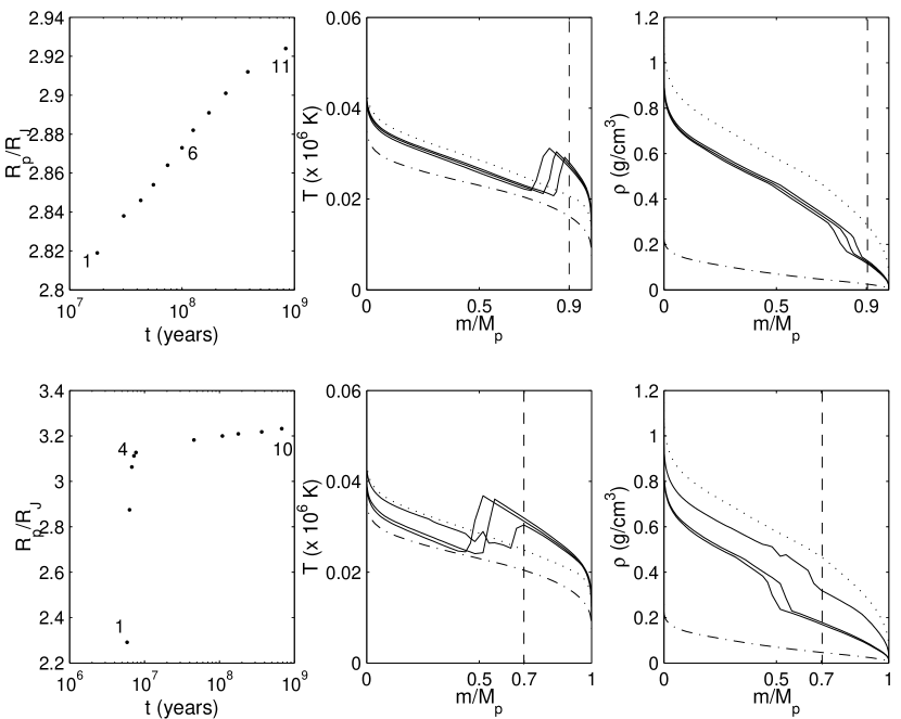
Figure 6: The evolution of $R_{p}$, the temperature profile, and the density profile for Models 11 (3 upper panels) and 12 (3 lower panels) in Table 2. While we only show the data after the planet has reached a quasi-thermal equilibrium in Model 11, in Model 12 the planet is not in the quasi-thermal equilibrium until the data point 4 (see the lower-left panel). The three solid curves from right to left in each of the temperature and density plots for Model 11 (Model 12) correspond to the three different stages marked by 1, 6, and 11 (1, 4, and 10) respectively in the $R_{p}$ vs $t$ plot. The vertical dashed lines in the temperature and density plots mark the location of the maximal heating of the Gaussian heating profile for Model 11 ($m_{0}/M_{p}=0.9$) and Model 12 ($m_{0}/M_{p}=0.7$). The temperature and density profiles for the uniform heating per unit mass represented by Model 9 (dash-dotted line) and for the surface heating denoted by Model 10 (dotted line) are also plotted for comparison.

Figure 6 displays the evolution of expansion for model 11 (upper panels) and model 12 (low panels). The three solid curves from right to left in each of the temperature and density diagrams are the profiles corresponding to the phases marked by the data points 1, 6, 11 in the $R_{p}$ vs $t$ diagram for model 11, and the phases labeled by the data points 1, 4, 10 in the $R_{p}$ vs $t$ diagram for model 12. The vertical dashed lines in the temperature and density diagrams denote the location of the center of the Gaussian heating zones: $m/M_{p}=0.9$ for model 11, and $m/M_{p}=0.7$ for model 12. In model 11, a heating front is generated at $m/M_{p}=0.9$ as is illustrated in the temperature diagram (i.e. the upper-middle panel) and then propagates inward. The front corresponds to the region with the temperature inversion. It also acts as a rarefaction structure as is shown in the density diagram. For comparison, we also draw the temperature and density profiles for model 9 (dot-dashed curves) and for model 10 (dotted curves). In model 12, a heating front is generated at $m/M_{p}=0.7$. As it travels inward (see the lower-middle panel), the front decreases the density analogous to a rarefaction wave (see the lower-right panel).

It is interesting to point out that except for the data points from 1 to 4 in model 12, all of the other data points in the $R_{p}$ versus $t$ diagrams correspond to a state of quasi-thermal equilibrium; i.e. the intrinsic luminosity $\cal L$ is equal to the dissipation rate. However the planet is not in a global thermal equilibrium because of the presence of a temperature inversion in the region just below the shell. This heat front very gradually propagates inward, and is associated with a gradual overall expansion. After quasi-thermal equilibrium is reached, the rate of expansion is very slow compared to its rate before this time (compare the data before and after point 4 in the lower left panel of Figure 6). Clearly, an analogous expansion phase does not occur in the uniformly heated case (model 9).

The underlying physical cause for expansion of $R_{p}$ without any gain of internal entropy (or very little gain of entropy as a result of the tail of a Gaussian profile) can be described as follows. Prior to reaching a quasi-thermal equilibrium, a giant planet experiences a fast inflation due to a high dissipation rate focused in a spherical envelope (such as the stage before the data point 4 for model 12 in Figure 6). In models 11 and 12, about 10% to 30% of planet gas by mass lies above the heating zone. This gas is inflated significantly due to a strong underlying shell-heating source as prescribed by the model. The huge inflation on the top of the heating shell reduces the pressure and therefore causes the whole region beneath the heating zone to expand and to adjust to a new hydrostatic equilibrium. The expansion induced by a shell-heating source is less efficient than that induced by a uniform heating throughout the envelope since more energy is radiated away for a given $R_{p}$, as we have already stated in the previous paragraph. The surface radiation becomes more intensified as the heating zone approaches to the photosphere.

After the entire shell-heated planet has reached its quasi-thermal equilibrium, the region around the heating front is not yet in the thermal equilibrium locally. This arises because the region just below the heating front (i.e. at the bottom of the temperature inversion region) gains entropy via convection from the bottom and through radiation from its top. But the region just above the heating front (i.e. at the top of the temperature inversion region) loses entropy due to radiation from its bottom and convection from its top. On the average, the net increase in entropy vanishes. Thus, the rarefaction heating wave is driven by a local entropy transport which averages to a zero net flux. Since the heating front is a result of the temperature inversion which transports entropy inward by radiative diffusion and causes the entropy disturbance, the time scale for the heating front to cross the planet’s interior is roughly equal to

$$t_{rarefaction} \sim {R_{p}\over\nu_{rad}/\Delta r}$$ (22)

$$\approx 40\left({R_{p}\over 3R_{J}}\right)\left({\Delta r\over 10^{8}\,{\rm cm}}\right)\left({3.5\times 10^{4}\,{\rm K}\over T}\right)^{3}\left({\kappa\over 10^{3}\,{\rm cm^{2}/g}}\right)\left({\rho\over 0.3\,{\rm g/cm^{3}}}\right)^{2}\left({c_{p}\over{\cal R}}\right)\ {\rm Gys},$$

where the radiative diffusivity $\nu_{rad}=4acT^{3}/3\kappa\rho^{2}c_{p}$, and $\Delta r$ is the width of the heating front. The reference values for $\Delta r$, $T$, $\kappa$, and $\rho$ shown in the above estimate are taken from the simulation for model 12. The large value of $t_{rarefaction}$ is consistent with our numerical results that the shell-heating planet expands very slowly after it has reached the quasi-thermal equilibrium (see the upper-left panel and the stage after the data point 4 in the lower-left panel in Figure 6). In reality the slow expansion of the planet due to the inward propagation of the rarefaction wave is unimportant, because the damping time for tidal dissipation is much short than $t_{rarefaction}$, and also $t_{rarefaction}$ is much longer than the lifetime of the star.

The ${\cal L}-R_{p}$ relation for model 12 before the planet reaches a quasi-thermal equilibrium can be fitted with a quadratic approximation:

$$\log({\cal L}/10^{27}\,{\rm erg/s})=-9.36888(\log R_{p}/R_{J})^{2}+11.9403(\log R_{p}/R_{J})-1.33544,$$ (23)

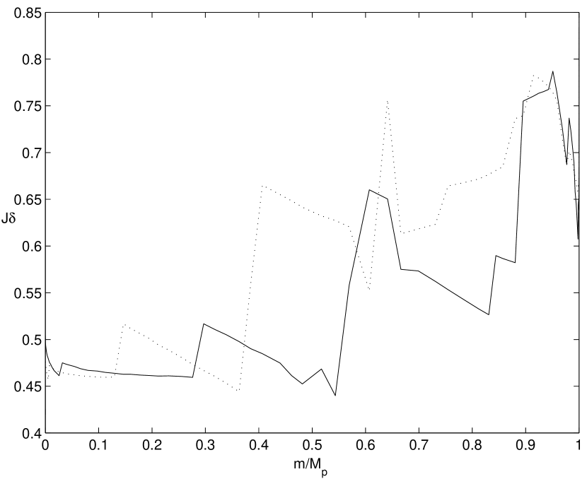
Figure 7: The radial profiles of $J\delta$ ($=1/\Gamma$) for the data point 1 (solid curve) and the data point 4 (dotted curve) in Model 12. The data points 1 and 4 are indicated on the lower-left panel in Figure 6. In Model 12, the energy is deposited in the shell of mass fraction $m_{0}/M_{p}=0.7$.

which indicates that $\gamma$ decreases with $R_{p}$ and $\gamma=5$ when $R_{p}=2.346R_{J}$. In contrast to the uniform heating cases, in which the planet’s interior gains entropy and expands, the degree of degeneracy at the planet’s center, in model 12, remains essentially constant ($D\approx 17$) during the evolution (see Figure 6). This tendency arises largely because the planet interior expands without gaining much entropy. This result implies that the flattening of $\cal L$ with $R_{p}$ in the shell-heating cases is not due to the reduction of electron degeneracy of the metallic interior, but is primarily caused by the gradual phase transformation from non-ideal properties to the ideal state within and above the shell-heating zone. This interpretation is well illustrated in Figure 7 in terms of $J\delta$ ($=1/\Gamma$, see equation (A19) and the description in Appendix) for the data point 1 (solid curve) and the data point 4 (dotted curve): while in the interior $J\delta$ hardly changes with $R_{p}$, $J\delta$ indeed increases with $R_{p}$ around and above the shell-heating zone.

4.2.2 Variations in other model parameters

In addition to the cases in which most of the dissipation is concentrated in a narrow spherical shell, we also considered the cases with relatively flat heating profiles for $\epsilon_{0}$. In Model 7 and 8, we choose the power index to be $\beta=2$. We found that the interior structure is almost the same for Models 7, 8, and 1. This similarity arises because the heating per unit volume $\rho\epsilon_{0}$ concentrated in the high-density inner region of the planet in all these models, including Model 7 with $\beta=2$. For much larger values of $\beta$, the internal structure of Model 7 and 8 should resemble that of Model 2 and 6 respectively.

Figure 8 depicts the density profiles of the planet in a thermal equilibrium with the regular and the reduced opacities for grains. The solid and dashed curves represent Models 1 and 4 respectively. In both models, $\kappa_{d}=\kappa_{0}$. The corresponding Models 13 and 14 for $\kappa_{d}=10^{-3}\kappa_{0}$ are marked with solid and dashed curves respectively. This reduction of opacity by a factor of $10^{3}$ is implemented in the grain region where $T<2100$ K. This region roughly corresponds to the radiative envelope of the planet. Since the radiative envelope is a bottleneck for the outward energy transport, the reduced opacity in the radiative envelope allows photons to escape from the planet much more easily. Consequently, the planet attains a much smaller size when a thermal equilibrium is established. The dashed curves have slightly smaller $R_{p}$ than the solid curves as a result of more radiative loss for the shell-heating cases as reasoned in the previous paragraph. Since the location of the heating shell is close to the planet’s center, the simulation for Model 15 is almost the same as that for Model 13.

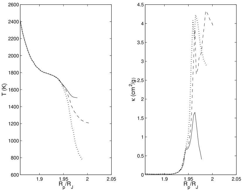
Figure 9: Temperature and opacity profiles in the radiative envelope for Model 1 (solid curve), Model 16 (dashed curve), and Model 17 (dotted curve). Different values of irradiation temperature are imposed here: $T_{0}=1500$ K for Model 1, $0.8T_{0}$ for Model 16, and $0.5T_{0}$ for Model 17.

We also computed the thermal equilibrium solution for models with different irradiation temperatures $T_{e}$. In Figure 9, we plot the temperature and opacity distributions for Models 1, 16, and 17 with solid, dashed, and dotted curves respectively. Since the interior structures for these three cases are almost the same, we only show the temperature and opacity profiles in the radiative envelopes, which are affected by the stellar irradiation. The planets with less irradiation (Models 16 & 17) have slightly larger equilibrium sizes than the one with more irradiation (Model 1). A direct comparison between Models 16 and 17 indicates that higher surface temperatures result not only in a slight increase in the density scale height of the planet’s atmosphere, but also an enhanced opacity. Both effects cause Model 16 to attain a larger $R_{p}$ than Model 17.

But $R_{p}$ for Model 1 is smaller than that for Model 16 even though the photospheric temperature for the former is higher than that of the latter. This difference arises because the temperature of the envelope in Model 1 is sufficiently high for most of the silicate grains to sublimate. Consequently, opacity in the radiative envelope in Model 1 is well below that in Model 16. The correlation between $R_{p}$ and $\kappa$ is already established in the previous discussion on Models 13–15. However, the difference in the size between Model 1 and Model 16 is only about 1%, in accord with the usual notion that the size of an optically-thick object should not be strongly altered by external irradiation.

4.2.3 Self consistent tidal heating models and inflation instability

We also consider, in Model 18, a self consistent calculation in which the energy dissipation is proportional to $R_{p}^{5}$ in accordance with equation (18). In this model, we assume that the energy dissipation is uniformly distributed in mass. The dissipation is normalized to $\epsilon_{0}=5\times 10^{-6}L_{\odot}$ at 2 Jupiter radii (this rate corresponds to $a=10R_{\odot}$ and $e\approx 0.18$ in equation (19). Note that $\tau_{R}\sim\tau_{d}$ in this case according to equation(21)). The final equilibrium size $R_{p}=1.857~{}R_{J}$ is slightly smaller than that ($R_{p}=1.977~{}R_{J}$) for Model 1. The planet would be slightly bigger ($R_{p}=1.983~{}R_{J}$) than that for Model 1 if the normalization constant were increased by 5%. Since $\gamma<5$ as $R_{p}\gtrsim 2R_{J}$, the planet is expected to be vulnerable to the tidal inflation instability once its size expands beyond $2R_{J}$. Our numerical results show that a further increase in the normalization constant by another 5% (therefore $e\sim 0.2$ and $\tau_{R}\sim 0.9\tau_{d}$ when $R_{p}=2R_{J}$ and $a=10R_{\odot}$ by equation(21)) causes $R_{p}$ to increase to at least 4 $R_{J}$.

In comparison to the uniform heating in Model 18, we consider in Models 19 and 20 the possibility of non-uniform heating with $m=0.9$ and $m=0.9999$, respectively. Similar to Model 18, the total heating rate is proportional to $R_{p}^{5}$. In Model 19 with the heating rate normalized to 2.1 times larger than $5\times 10^{-6}L_{\odot}$ at $R_{p}=2R_{J}$ (this corresponds to $e\approx 0.26$ at $a=10R_{\odot}$ according to equation (19)), the planet is thermally unstable and swells from 2$R_{J}$ to 3$R_{J}$ in about 2 Myrs (shorter than the eccentricity damping time scale $\tau_{d}\approx 2.7$ Myrs according to equation (20) evaluated at $R_{p}=3R_{J}$). When the heating rate is normalized to 4 times larger than $5\times 10^{-6}L_{\odot}$ at $R_{p}=2R_{J}$ (this corresponds to $e\approx 0.07$ at $a=0.03$ AU according to equation(19)) in Model 19, the planet is thermally unstable and expands from 2$R_{J}$ to 3$R_{J}$ in about 0.27 Myrs (the eccentricity damping time scale $\tau_{d}\approx 0.15$ Myrs and 1.17 Myrs evaluated at $R_{p}=3R_{J}$ and $R_{p}=2R_{J}$, respectively).

When the normalized heating is set to be $10^{-3}L_{\odot}$ for $a=0.03$ AU and $R_{p}=2R_{J}$, equation (19) is no longer a fair approximation and equation (27) in paper II gives $e\approx 0.294$ for this heating rate. In this case the planet with or without a core expands from $2~{}R_{J}$ to $3.6~{}R_{J}$ in less than 40000 years which is shorter than the eccentricity damping time $\approx 47800$ years for $R_{p}=3.6~{}R_{J}$ according to equation (12) in paper II. Since the planet’s size $3.6~{}R_{J}$ is actually beyond the Roche radius $R_{L}\approx 3~{}R_{J}$ for $a=0.03$ AU and $e=0.294$, the inflated planet would overflow the inner Lagrangian point in this case.

The expansion rate is drastically reduced for Model 20 in which the dissipation is largely deposited at $m=0.9999$, roughly the location of the radiation-convection boundary. A one-Jupiter mass planet with the normalized heating $5\times 10^{-6}L_{\odot}$ at $R_{p}=2R_{J}$ can only reach the final size of $\approx 1.9~{}R_{J}$. A normalized heating rate which is twice as big as $5\times 10^{-6}L_{\odot}$ results in a final size $\approx 1.95~{}R_{J}$. The planet with the normalized heating four times as large as $5\times 10^{-6}L_{\odot}$ in Model 20 expands very slowly to $2~{}R_{J}$ from $1.9~{}R_{J}$ over several tens of million years, which is comparable with the eccentricity damping time scale 20 Myrs at $a=10R_{\odot}$ and is much longer than the eccentricity damping time scale ($\simeq$ 1.17 Myrs) at $a=0.03$ AU. The planet in Model 20 obviously requires a larger normalized heating rate than Model 19 to reach the critical size beyond which the planet is thermally unstable in response to the $R_{p}^{5}$ heating rate.

5 Summary and discussion

In this paper, we continue our investigation on the adjustment of a planetary interior as a consequence of intense tidal heating. As a giant planet’s interior is heated and inflated, we showed in Paper II that its interior remains mostly convective. Efficient energy transport leads to an adiabatic stratification. With a constant heating rate per unit mass, we deduced an unique luminosity-radius relation regardless of how intense the heating rate is. The planet’s luminosity increases with its radius. But the growth rate of $\cal L$ is a decreasing function of $R_{p}$. At the same time, the tidal dissipation heats the interior of the planet at a rate which increases rapidly with $R_{p}$. At around $2~{}R_{J}$, $\cal L$ can no longer sustain sufficient growth to maintain a thermal equilibrium with the tidal dissipation rate. Thereafter, the planet’s inflation become unstable and it overflows its Roche radius and become tidally disrupted.

Here we show that the change of luminosity during the planet’s expansion is directly linked to the evolution of its interior, in particular, the equation of state. We employ the polytrope approach to investigate the interior structure of an inflated giant planet. According to the simulation, interior profiles deviate away from $P\propto\rho^{2}$ as the planet expands. The central temperature $T_{c}$ increases and then decreases with the size of the planet. Also $P_{c}$ and $\rho_{c}$ are less steep functions of $R_{p}$ than the polytrope theory with a constant polytropic index $n$ indicates. All of these effects suggest that the planet interior does not evolve in a self-similar manner, but $n$ gets larger as $R_{p}$ increases. In conjunction with the numerical results that the degeneracy $D$ decreases, and that $T_{c}$ rises and then drops during the course of inflation, the result of a positive value of $dn/dR_{p}$ can be interpreted as a manifestation of a reduction in degeneracy during the expansion.

We reason that the coefficient of thermal expansion $\delta$ increases in response to a decrease in degeneracy and non-ideal effects, leading to an increase in $n$ through equation (A19). Consequently the planet compressibility at constant mass $C_{M}$ increases with $R_{p}$ (see equation A21). This pattern can be translated into the phenomenon of a decrease in luminosity growth during the inflation, as a consequence of an one-to-one relation between $K$ and $\cal L$ in the case of uniform heating in mass under the conditions of the polytropic interior and hydrostatic equilibrium. We also compare the results between a planet with a core and without a core. To be inflated to the same size, a planet with a core, therefore possessing a larger gravitational binding energy, needs a larger intrinsic luminosity $\cal L$ than a planet with no core and the same mass. We also show that the opacity in the radiative envelope has a drastic effect on the final equilibrium size of an inflated planet: the size would be much smaller if grains are depleted in the radiative envelope.

We also consider the possibility of localized tidal dissipation. Such a process may occur in differentially rotating planets or near the interface between the convective and radiative zones where the wavelength associated with dynamical tidal response is comparable to the density scale height. Localized dissipation may also occur through the dissipation of resonant inertial waves or radiative damping in the atmosphere. In the strong shell-heating models, the one-to-one relation between $K$ and $\cal L$ disappears because of the existence of a radiative region caused by temperature inversion beneath the shell-heating zone. The unheated planet’s interior in such cases might still be inflated due to a significant expansion of the gas above the heating zone, although the overall expansion rate is less efficient than that in the uniform heating cases as a result of a greater amount of radiative loss from the planet’s photosphere. Without gaining entropy, the expanding interior cannot lift its degeneracy and therefore cannot increase its elasticity. However, the gas above the shell-heating zone can lift its non-ideal properties and hence enhance its elasticity, leading to a decrease in $\Gamma$ in that region and thereby diminishing the growth rate of $\cal L$ as the planet expands.

Finally, we consider the self consistent response, taking into account the modification of heating rate due to a planet’s expansion. In this paper, we adopt a constant-$Q$ prescription for equilibrium tides in which the tidal dissipation rate is assumed to be proportional to $R_{p}^{5}$. The results for the uniform heating model suggest that a young gaseous planet of $1~{}M_{J}$ without a solid core can be thermally unstable and inflated from $2~{}R_{J}$ to a size beyond $4~{}R_{J}$ if $e\sim 0.2$ at $a=10~{}R_{\odot}$. If the dissipation rate is proportional to $R_{p}^{5}$, and if most of the tidal perturbation is deposited at $m/M_{p}=0.9$, a core-less young planet of $1M_{J}$ would be thermally unstable and inflated from $2R_{J}$ to a size beyond $3R_{J}$ for $e>0.07$ at $a=0.03$ AU or $e>0.26$ at $a=10R_{\odot}$.

With the same heating concentration $m/M_{p}=0.9$ and $R_{p}$-dependence in the dissipation rate, a young planet with a core at $a=0.03$ AU with an initial eccentricity $e>0.294$ can be inflated from $2~{}R_{J}$ to a size beyond its Roche radius. We have assumed that the convective flow still behaves adiabatically even though the heating shell causes a narrow radiative zone. However, the condition away from adiabaticity implies that the internal heat is not transported away as efficiently as in the case of adiabatic convection, leading to a more severe reduction in non-ideal properties of the gas and therefore an even faster decrease of $\gamma$ as the planet expands.

Note that the Eddington approximation for the surface boundary condition is used in these models rather than more detailed frequency-dependent model atmospheres. This approximation is not necessarily valid for the strongly irradiated atmospheres studied here (Guillot & Showman (2002)). However it is unlikely to make much difference for the main results discussed here, namely the behavior of the planet’s radius as a function of tidal dissipation energy. It could, however, lead to errors in other kinds of predictions, such as the radius as a function of opacity.

The equilibrium tidal dissipation formula is based on an ad hoc assumption of a constant lag angle. In reality, the dynamical tidal response of a planet through both gravity and inertial waves near the planet’s surface and convective envelope may be much more intense, especially through global normal modes. Their dissipation may provide the dominant angular momentum transfer mechanism for the orbital evolution and heating sources for the internal structure of close-in extrasolar planets. In the limit of small viscosity, the intensity of tidal dissipation is highly frequency dependent (Ogilvie & Lin 2004). When the forcing and response frequencies are in resonance, the energy dissipation rate is intense whereas between the resonances it is negligible. As the planets undergo structure adjustments, their spin frequency, Brunt–Väisälä frequency distribution, the adiabatic index, and equation of state also evolve. Since all of these physical effects contribute to the planets’ dynamical response to the tidal perturbation from their host stars, their response and resonant frequencies are continually modified. The results in this paper indicate that the structure of the planet adjusts on a radiation transfer time scale which generally differs from the time scale for a planet to evolve through the non resonant region. In addition, the tidal forcing frequency also changes as the planets evolve toward a state of synchronous spins and circular orbits. Therefore, it is more appropriate to consider a frequency averaged tidal dissipation rate. In the limit of small viscosity, the frequency averaged dissipation rate converges (Ogilvie & Lin 2004) such that the equilibrium tidal dissipation formula may be a reasonable approximation. Nevertheless, we cannot yet rule out the possibility that some close-in planets may attain some non resonant configuration and stall their orbital evolution. Therefore, accurate measurement of the sizes of close-in young Jupiters via planet transit surveys can be used to constrain the theories of tidal dissipation and hence internal structure for these objects.

Appendix A A Polytrope Model

In order to identify the dominant physical effects which determine the internal structure of planets, we consider an inflated giant planet that consists of a polytropic interior and a thin envelope. With this model we can construct analytic solutions. For this analysis, we assume that the polytropic interior comprises almost all of the mass and radius, and that the thin envelope overlying the interior is radiative and is composed of a non-degenerate ideal gas. Therefore, the polytropic equation $P=K\rho^{1+1/n}$, together with the condition for hydrostatic equilibrium, specifies the value of $K$ for a given planet’s mass $M_{p}$ and a given planet’s size $R_{p}$ (Cox & Giuli (1968)):

$$K=k_{n}M_{p}^{1-1/n}R_{p}^{-1+3/n},$$ (A1)

where $k_{n}$ is a function of $n$. All of thermodynamic quantities must be continuous across the boundary between the convective interior and the radiative envelope, such that

$$P_{b}={{\cal R}\rho_{b}T_{b}\over\mu}$$ (A2)

$$P_{b}=K\rho_{b}^{1+1/n}$$ (A3)

$$\nabla_{polytrope}=\nabla_{rad}\approx{3\over 16\pi acG}{P_{b}\kappa_{b}\over T_{b}^{4}}{{\cal L}\over M_{p}},$$ (A4)

where the subscript $b$ denotes the values evaluated at the boundary. The magnitude of $\nabla_{polytrope}$ is determined by the equation of state of the gas in the interior such that it is a function of $n$ rather than directly dependent on the magnitude of $R_{p}$ and $M_{p}$. Note that in equation (A4) we have assumed that $\cal L$ does not vary greatly across the radiative envelope after it emerges from the polytropic interior. This assumption should be a reasonable approximation for the thin radiative envelope so long as there is no localized source of intense heating there. The above four equations give rise to the relation

$${\cal L}\propto{M_{p}T_{b}^{3}\over\rho_{b}\kappa_{b}}\propto{k_{n}^{n}M_{p}^{n}(T_{b}R_{p})^{3-n}\over\kappa_{b}}\left({\mu\over{\cal R}}\right)^{n},$$ (A5)

where ${\cal R}$ is the gas constant and $\mu$ is the mean molecular weight. From the opacity table, we find that the opacity at the boundary may be roughly approximated by a power law

$$\kappa_{b}\propto{T_{b}}^{a},$$ (A6)

with $a=4.08$.

A.1 Completely Degenerate Interior

The equation of state for a completely degenerate gas in the non-relativistic regime is given by $P\propto\rho^{5/3}$, which corresponds to the $n=3/2$ polytrope with a constant $K$. Therefore, equation (A1) leads to the well-known mass-radius relation for low-mass white dwarfs:

$$R_{p}\propto M_{p}^{-1/3},$$ (A7)

which does not vary with ${\cal L}$. This independence is equivalent to the expression

$$\gamma\equiv{d\ln{\cal L}\over d\ln R_{p}}\rightarrow\infty.$$ (A8)

A.2 Partially Degenerate Interior with $n=1$ Polytrope

We now consider a model in which the planet has a sufficiently large $R_{p}$ such its interior is partially degenerate with an $n=1$ equation of state ($P\propto\rho^{2}$). Partial degeneracy occurs when $D\approx 1$. Therefore by setting $D=1$ in equation (12), the partially degenerate interior can be described by

$$\rho=cT^{3/2},$$ (A9)

where $c$ is a constant. Under these conditions, $\nabla_{ad}=1/3$, which is consistent with the numerical solution for the region dominated by the pressure-ionized hydrogen atoms as shown in Figure 2.

At the boundary, equations (A1), (A2), (A3), and (A9) uniquely determine the value of $T_{b}$ for a given planet’s size $R_{p}$ without having to consider the photosphere:

$$T_{b}=\left({{\cal R}\over\mu}\right)^{2}{1\over K^{2}c^{2}}=\left({{\cal R}\over\mu k_{1}}\right)^{2}{1\over R_{p}^{4}c^{2}}\approx 2300\,{\rm K}\left({2R_{J}\over R_{p}}\right)^{4}\left({2\times 10^{-7}{\rm g\,cm^{-3}\,K^{-3/2}}\over c}\right)^{2}\left({1\over\mu}\right)^{2}.$$ (A10)

With equations (A5) and (A6), it follows that

$${\cal L}\propto M_{p}R_{p}^{10.32}c^{4.16}.$$ (A11)

Figure 3 shows that the degree of degeneracy at the center of the planet decreases from 21 to 9 as its radius expands from 1.777 $R_{J}$ to 2.826 $R_{J}$. The value $c$ decreases as the degree of partial degeneracy is reduced ($c\approx 6\times 10^{-9}$ g cm^-3 K^-3/2 when Fermi energy equals thermal energy). Therefore, in accordance with equation (A9), the temperature of the planet can increase with, even though $\rho$ decreases with, $R_{p}$. Temperature indeed increases until $R_{p}$ is increased up to $\approx 2.3R_{J}$. The temperature then decreases with $R_{p}$ after that, as seen in our numerical results.

Figure 10 depicts the coefficient of thermal expansion at constant pressure $\delta$ $(\equiv-(\partial\ln\rho/\partial\ln T)_{P})$, $\chi_{T}$ ($\equiv(\partial\ln P/\partial\ln T)_{\rho}$), and $J\delta$ (related to the adiabatic index, see eq(A18)) for a planet of $0.63M_{J}$ as a function of the co-moving mass coordinate $m/M_{p}$. The boundaries $m/M_{p}=0$ and $m/M_{p}=1$ represent the location of the planet’s center and its photosphere, respectively. The curves in Figure 10 are not smooth because the calculation involves several numerical derivatives. The magnitude of these thermal expansion coefficients decreases as the gas changes its phase from the ideal to the non-ideal regime, and approach to zero as a fluid increases its degeneracy, meaning that $PdV$ work is of less importance in a more degenerate gas as indicated in equation (5). Figure 10 shows that $\delta$ and $\chi_{T}$ monotonically increase with $m/M_{p}$, resulting from a transition from partial degeneracy in the inner region featuring the pressure-ionized hydrogen gas, to the non-ideal phase of dense molecular hydrogen in the middle range of $m/M_{p}$, and then to the ideal-gas regime in the very outer region (not able to be shown because of the small scale) where $\delta=\chi_{T}=1$. The magnitudes of $\delta$ and $\chi_{T}$ are larger in the case of a relatively large size planet (with $R_{p}=3.22R_{J}$) because the equation of state for its interior is less degenerate and more ideal than that for a smaller planet (with $R_{p}=1.66R_{J}$). This correlation is consistent with the consequence that the temperature variation results from the shift of degeneracy. Since $c$ drops as $R_{p}$ increases, the term $c^{4.16}$ in equation (A11) indicates that the exponent of $R_{p}$ should become less than 10.32 as the degree of partial degeneracy is reduced.

A.3 Adiabatic interior composed of an ideal gas

For planets with extremely large $R_{p}(>>2R_{J})$, the density near the center of the planet become sufficiently low that degeneracy is lifted and the equation of state is better approximated by that of an ideal gas for an $n=1.5$ polytrope. In this limit, the radiative envelope is also relatively extensive. Integrating the radiative diffusion equation over the radiative envelope, we find the ratio of the temperature at the boundary $T_{b}$ to the temperature at the photosphere $T_{ph}$ (Cox & Giuli (1968)) to be

$${T_{b}\over T_{ph}}=\left({(1+n_{eff})\nabla_{ph}-1\over(1+n_{eff})\nabla_{ad}-1}\right)^{1\over m+s+4},$$ (A12)

where $\kappa\propto\rho^{m}T^{-s}$, $n_{eff}=(s+3)/(m+1)$, and the value of $\nabla$ at the photosphere

$$\nabla_{ph}\equiv{3\over 16\pi acG}{P_{ph}\kappa_{ph}\over T_{ph}^{4}}{{\cal L}\over M_{p}}={1\over 8}{{\cal L}\over 4\pi R_{p}^{2}\sigma T_{ph}^{4}}.$$ (A13)

In deriving the above equation, we have used $P_{ph}=2GM_{p}/3R_{p}^{2}\kappa_{ph}$. Since ${\cal L}$ is usually much smaller than the stellar irradiation $4\pi R_{p}^{2}\sigma T_{ph}^{4}$ and therefore $\nabla_{ph}<<1$, the ratio $T_{b}/T_{ph}$ is not a sensitive function of ${\cal L}$ and $M_{p}$. Since $T_{ph}$ is determined by the stellar irradiation, neither it nor $T_{b}$ varies significantly with ${\cal L}$ and $M_{p}$.

There are some uncertainties for the values of $m$ and $s$. If we evaluate $\kappa$ for the radiative/convective interface, we find from equation (A6) that $m=0$ and $s=-4.08$. The temperature near the surface layer is 2000-3000 K such that the diatomic molecular hydrogen attains $n=5/2$ and $\nabla_{ad}=2/7$. With these parameters, we find from equation (A12), $T_{b}\approx 1.326T_{ph}\approx 2150$ K when $T_{ph}=1620$ K. Near the photosphere, the grains may also provide the dominant opacity source, in which case $s=-1$ but other parameters have the same values. In this case, we find from equation (A12) that $T_{b}\approx 1.91T_{ph}\approx 3090$ K which is too high for grain opacity to be relevant. The actual values of $s$ and $T_{b}$ are probably between these extreme cases. Finally, with equations (A5) and (A6) we find for $n=5/2$, an ideal-gas equation of state leads to

$${\cal L}\propto M_{p}^{5/2}R_{p}^{1/2}.$$ (A14)

A.4 Polytropic evolution and planet compressibility

As we can see clearly from equations (A8), (A11), and (A14), the values of $\gamma$ decrease from $\infty$ to 10.32 to 0.5 as the degeneracy is lifted for increasing values of $R_{p}$. The physical properties responsible for this change can be attributed to the “compressibility” of the planet. It is well known that the compressibility of a gas is linked to the effective exponent $\Gamma_{eff}\equiv d\ln P/d\ln\rho$ which varies with different thermal conditions in a situation of thermal equilibrium. However, in the case of inflated giant planets, $\Gamma_{eff}$ is always equal to the adiabatic value $\Gamma_{ad}=(d\ln P/d\ln\rho)_{ad}$ due to an efficient energy transport by convection. Consequently, $\Gamma_{eff}$ varies with different equations of state which are characterized by the index of polytrope $n$ in our case. We shall elucidate this point in this section.

In general, equations (A5) and (A6) can be approximated with a simple relation

$${\cal L}\propto{M_{p}\over\rho_{b}T_{b}}.$$ (A15)

The factor $M_{p}$ comes into the above expression because the larger $M_{p}$ is, the larger gravity is in the thin radiative envelope, and therefore the stronger $\cal L$ is due to the steeper temperature gradient in the radiative envelope. Unlike the relation with $M_{p}$, $\cal L$ decreases as $\rho_{b}$ increases simply because the radiative energy flux decreases as the density and therefore the optical depth increase.

The numerical solutions for the constant $\epsilon$ models show that $T_{b}$ increases with $R_{p}$ when the degree of partial degeneracy is relatively high. But $T_{b}$ decreases with $R_{p}$ when the degree of partial degeneracy is modest ($R_{p}$ is larger than 2.3 $R_{J}$). This tendency suggests that $T_{b}$, a thermal quantity introduced by the equation of state in the framework of a polytropic analysis, primarily varies with $c$ as shown in equation (A9).

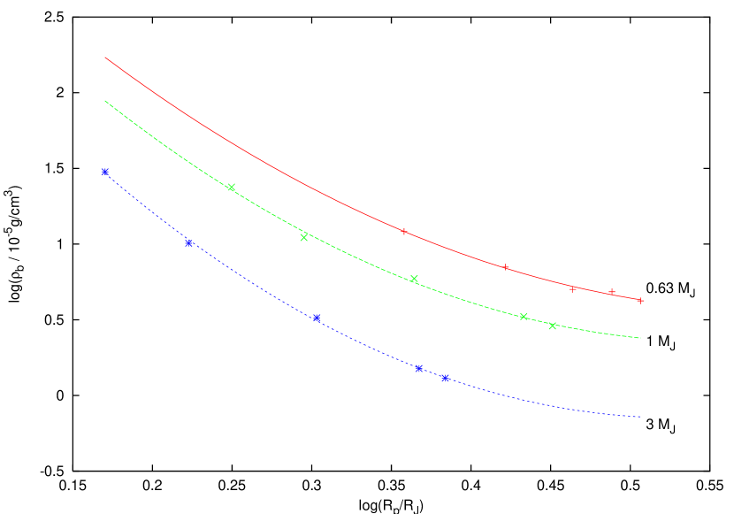
Figure 11: The density at the interface between the radiative envelope and the convective interior $\rho_{b}$ as a function of the planet’s radius $R_{p}$. While discrete points are the simulation data, the fitting curves are illustrated by a solid line ($0.63M_{J}$), a dashed line ($1M_{J}$), and a dotted line ($3M_{J}$).

Figure 11 illustrates the mass density at the interface between the radiative envelope and the convective interior, $\log\rho_{b}$ as a function of the planet size $\log R_{p}$. As the planet expands, $\log\rho_{b}$ decreases but its slope gets flattened. The similarity between Figure 11 and 1 suggests that the flattening of $\log\rho_{b}$ is the major cause of the flattening of $\log{\cal L}$ as the planet is inflated. Equation(A5) implies that

$$\rho_{b}\propto T_{b}^{n}M_{p}^{1-n}\left({R_{p}^{n-3}\over k_{n}^{n}}\right)\left({{\cal R}\over\mu}\right)^{n}.$$ (A16)

As demonstrated in Figure 4, the simulation shows that the fraction of the volume of the planet which deviates from the $n=1$ polytrope increases with $R_{p}$. This dependence is roughly equivalent to the polytropic index being an increasing function of $R_{p}$. We fit the curves in the region of convection zones in Figure 4 for the core-less cases with a polytropic index and show the results in Table 1. The terms $({\cal R}/\mu)^{n}$ and ${k_{n}}^{n}$ in the above equation increase with $n$, but their influence is much weaker than the terms $R_{p}^{n-3}$ and ${M_{p}}^{1-n}$ because $R_{p}$ and $M_{p}$ are much larger. As a result, the simple polytropic approach roughly suggests that ${\cal L}\propto{R_{p}}^{3-n}{M_{p}}^{n}$, and hence the value of $\gamma$ (as defined by eq. A8) decreases with $R_{p}$ as $3-n$ decreases with $R_{p}$. Equation(A5) gives a more precise representation of $\gamma$ as a function of $R_{p}$:

$${d\gamma\over d\log R_{p}} = 2{dn\over d\log R_{p}}\left({d\log k_{n}\over d\log R_{p}}-{d\log T_{b}\over d\log R_{p}}-1\right)$$ (A17)

$$+ n{d^{2}\log k_{n}\over d(\log R_{p})^{2}}-(a-3+n){d^{2}\log T_{b}\over d(\log R_{p})^{2}}+{d^{2}n\over d(\log R_{p})^{2}}\log\left({M_{p}k_{n}\mu\over R_{p}{\cal R}T_{b}}\right)$$

$$\approx -2{dn\over d\log R_{p}}.$$

The approximations made for the last expression in the above derivation are that we ignore the terms associated with the 2nd derivative with respect to $\log R_{p}$, and that the terms $d\log k_{n}/d\log R_{p}$ and $d\log T_{b}/d\log R_{p}$ are less than unity.

The magnitude of ${\cal L}$ increases with $M_{p}$ for a given $R_{p}$ as suggested by the factor ${M_{p}}^{n}$, which is consistent with the results shown in Figure 1. An increase of $n$ with $R_{p}$ in the polytropic analysis can be affirmed by the numerical results which show that the central density $\rho_{c}$ and the central pressure $P_{c}$ do not scale as fast as $R_{p}^{-3}$ and $R_{p}^{-4}$ respectively. But, $\rho_{c}\propto R_{p}^{-1.6}$ and $P_{c}\propto R_{p}^{-2.24}$, i.e. the ratio of the central density to the average density $\rho_{c}/<\rho>$ increases with $R_{p}$, meaning that $n$ also increases with $R_{p}$. Hence, the fact that an inflating planet loses its partial degeneracy can be interpreted as an increase of $n$ from 1 in the polytropic analysis. The overall effect on the intrinsic luminosity $\cal L$ for its dependence on $R_{p}$ is that $\gamma$ ($\equiv d\ln{\cal L}/d\ln R_{p}$) decreases with $R_{p}$ due to the flattening of the value of $\rho_{b}T_{b}$ as the planet inflates and loses its degeneracy.

Another piece of information which suggests a correlation between electron degeneracy and $\gamma$ is the comparison of the evolution of $\gamma$ between the core and core-less cases. As shown in §3, $\gamma$ passes 5 at a smaller $R_{p}$ for a less massive planet ($M_{p}=0.63$, $1M_{J}$) with a core than for that without a core. In the case of a less massive planet, a planet with a core requires more internal heating (see Fig. 1) than that with no core to be inflated to the same size, resulting in a lower degeneracy of the planet interior and therefore a faster decrease in $\gamma$ even though the core does not expand at all and the planet with a core is more gravitationally bound. On the other hand, $\gamma$ decreases below 5 when $R_{p}$ expands beyond $2.243R_{J}$ for a massive planet ($M_{p}=3M_{J}$) in both core and core-less cases. The reason for this independence of the core structure is because a $3M_{J}$ planet without a core has a central density comparable to the 5 g/cm³ which we impose for the density of the core in our numerical prescription; i.e. the interior structure of a massive core-less planet is comparable to that of the planet with a core, resulting in the similar $\cal L$ and $D$ required for the core and core-less cases to be inflated to the same size (see Fig. 1). In summary, given a size of an inflated less massive giant planet and assuming that the core is not heated and does not radiate, the planet with a core is less degenerate than the one without a core, and hence the planet with a core has a smaller $\gamma$ and expands more for a given amount of entropy input (see equation (A21) and detailed explanations below).

If we trace back through the above derivation, we note that the relation ${\cal L}\propto{R_{p}}^{3-n}{M_{p}}^{n}$ originates from equation (A1). The parameter $K$ might be related to the total entropy content of a polytropic object. The energy equation can be expressed as follows (Kippenhahn & Weigert (1990)):

$$ds=c_{p}J\left(d\ln P-{1\over J\delta}d\ln\rho\right),$$ (A18)

where $J\equiv-\nabla_{ad}+1/\chi_{T}$ and $\chi_{T}\equiv(\partial\ln P/\partial\ln T)_{\rho}$. Therefore the adiabatic exponent $\Gamma$ and the polytropic index might be written in terms of $\delta$ and $\chi_{T}$:

$$1+{1\over n}=\Gamma={1\over J\delta}.$$ (A19)

For a completely degenerate gas, $\chi_{T}\rightarrow 0$, $\delta\rightarrow 0$, and $1/J\delta$ can be written as the expression $d\ln P/d\ln\rho$ which equals 5/3 in the non-relativistic case. As the degree of degeneracy is reduced, both $\delta$ and $\chi_{T}$ increase away from zero, and $J$, whose evolution is dominated by $1/\chi_{T}$, decreases from infinity. In the region of the middle and larger values of $m/M_{p}$ where molecular hydrogen is abundant, both $\delta$ and $\chi_{T}$ increase with $R_{p}$ as the non-ideal effect is lifted (Saumon et al. (1995)). This qualitative evolution of $\delta$ and $\chi_{T}$ is in agreement with the plots obtained for a simulation with an inflated planet of 0.63 $M_{p}$ (first two panels in Figure 10). The third panel in Figure 10 shows that the evolution of the product $J\delta$ is dominated by $\delta$ and therefore increases as the planet expands, leading to an increase in the polytropic index $n$.

Motivated by the entropy equation (A18), which indicates that the specific entropy $s\propto\ln(P/\rho^{\Gamma})=\ln K$, we associate the issue of entropy to the polytropic approach with a constant $n$ by re-writing equation (A1) as

$$d\ln R_{p}=C_{M}d\ln K+C_{K}d\ln M_{p},$$ (A20)

where we have defined the compressibilities $C_{M}$ at constant mass and $C_{K}$ at constant entropy as follows

$$C_{M} \equiv \left({d\ln R_{p}\over d\ln K}\right)_{M_{p}}={n\over 3-n},$$ (A21)

$$C_{K} \equiv \left({d\ln R_{p}\over d\ln M_{p}}\right)_{K}={1-n\over 3-n}.$$ (A22)

For a completely degenerate gas, $K=$constant (hence the result $n/(3-n)$ shown in eq. (A21) breaks down), $C_{K}=-1/3$ (since $n=1.5$), and the term associated with $C_{M}$ vanishes in the non-relativistic case. In the cases of terrestrial planets and asteroids where the atomic/molecular interaction dominates and therefore the density is on the similar order regardless of mass, volume, and entropy, the interior structure can be roughly described by the $n=0$ polytrope. When $n=0$, $C_{K}=1/3$, $C_{M}=0$ and $\Gamma=\infty$. These relations reflect a nearly constant density ($C_{K}=1/3$) for the planetary interior as well as the difficulty of producing any non negligible density gradient with an entropy ($C_{M}=0$) and gravity ($\Gamma=\infty$) distribution. In the special case of partial degeneracy, $C_{K}\simeq 0$ and $C_{M}$ increases as $n$ rises from 1. The zero value of $C_{K}$ indicates a maximum size of the planet at $n=1$ solely in response to the mass change (Hubbard (1984)). Phenomenologically this result arises from a transition from degeneracy ($M_{p}\propto R^{-3}$) to the non-ideal equation of state ($M_{p}\propto R^{3}$) due to atom-atom/molecule-molecule repulsion (Burrows et al. (2001); Shu (1992)). In terms of the polytropic index, the state of partial degeneracy with $n\approx 1$ is just a transition from an $n=3/2$ degenerate state to an $n=0$ constant-density state. The rise of $C_{M}$ with $n$ means that, for a given mass, the rate of $R_{p}$ change in response to the change of total entropy gets more sensitive as $n$ increases, leading to the radius-adiabat relation and therefore the radius-luminosity relation for constant heating per unit mass.

It is physically straightforward to see why $C_{M}$ increases with $n$ and (therefore decreases with $\Gamma$). It is because the adiabatic exponent $\Gamma=\Gamma_{ad}$ is just the bulk modulus for adiabatic expansion/compression. Equation (A21) can be re-arranged to have the following form:

$${1\over C_{M}}=3(\Gamma-\Gamma_{M_{p}}),$$ (A23)

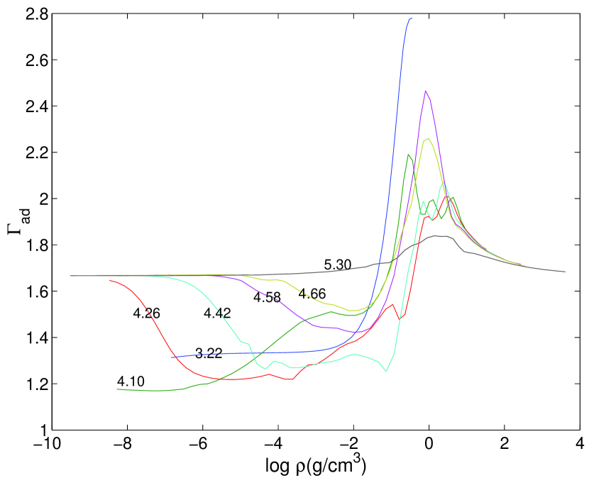
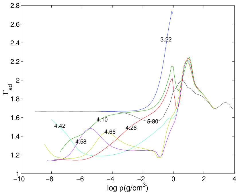
Figure 12: $\Gamma_{ad}$ as a function of $\log\rho$(g/cm³) and $\log T$(K) for hydrogen (left panel) and for helium (right panel). The number marked on each curve denotes $\log T$(K).

where we have defined the bulk modulus at constant planet’s mass $\Gamma_{M_{p}}\equiv(\partial\ln P_{c}/\partial\ln\rho_{c})_{M_{p}}$ which equals the constant 4/3. The adiabatic bulk modulus $\Gamma_{ad}$ should decrease as the planet’s elasticity $C_{M}$ increases due to the reduction of electron degeneracy and non-ideal effects. Figure 12 illustrates the isothermal curves for $\Gamma_{ad}$ as a function of $\log\rho$ in the case of hydrogen (left panel) and helium (right panel). The number marked on each curve denotes the logarithmic value of temperature $\log T$(K). The plots are drawn based on the tabulated equations of state (Saumon et al. (1995)). The peaks of $\Gamma_{ad}$ ($\approx 2$) around $\rho\gtrsim 1$ g/cm³ at the temperature $T\sim 10^{4}$–$10^{5}$K roughly correspond to the pressure-ionized regime of a Jupiter interior. This effect may be compared to the sudden rise of $\Gamma_{ad}$ for $\log T$(K)$=3.22$ at high densities as a result of non-ideal effects in the dense molecular (for hydrogen) or atomic (for helium) regime (also see Figs. 8 & 15 in Saumon et al. (1995)). The variation of $\chi_{\rho}\equiv\partial\log P/\partial\log\rho|_{T}$ and of $\Gamma_{ad}$ are quite similar; the rise of $\Gamma_{ad}$ in the pressure-ionized phase in the case of higher temperatures should also result from the non-ideal effects due to the interactions between densely-packed hydrogen and helium atoms, increasing the rigidity of the fluid. After all, equation (A20) describes the simple fact that the size of a planet is in general determined by its gravity ($M_{p}$), its entropy content ($K$), and the elastic properties of the planet responding to gravity (described by $C_{K}$) and to the entropy content (quantified by $C_{M}$).

Table 1: Polytropic Fitting for An Inflated Giant Planet of 1$M_{J}$ Without A Core

$R_{p}/R_{J}$	1.777	1.973	2.314	2.711	2.826
$n$	2.058	2.141	2.222	2.358	2.392
$({k_{n}})^{n}$	0.098	0.102	0.107	0.118	0.122

Table 2: Parameters for various models: $\epsilon_{s}=5\times 10^{-6}L_{\odot}$, $M_{p}=1M_{J}$, and $T_{0}=1500$ K. The last column entitled “figure” shows the figures, in terms of their labels, in which the model is plotted. For instance, Model 1 appears in Figures 5, 8, and 9.

Model	$\epsilon$	${\epsilon_{0}\over\epsilon_{s}}$	$\beta$	${m_{0}\over M_{p}}$	${\Delta m\over M_{p}}$	${\kappa_{d}\over\kappa_{0}}$	${T_{e}\over T_{0}}$	figure
1	$\epsilon_{1}$	1	0	-	-	1	1	5, 8, 9
2	$\epsilon_{3}$	1	-	0.9999	0.00015	1	1	5
3	$\epsilon_{3}$	1	-	0.95	0.05	1	1	-
4	$\epsilon_{3}$	1	-	0.90	0.05	1	1	8
5	$\epsilon_{3}$	1	-	0.70	0.05	1	1	5
6	$\epsilon_{3}$	1	-	0.05	0.05	1	1	5
7	$\epsilon_{1}$	1	2	-	-	1	1	-
8	$\epsilon_{2}$	1	2	-	-	1	1	-
9	$\epsilon_{1}$	10	0	-	-	1	1	6
10	$\epsilon_{3}$	10	-	0.9999	0.05	1	1	6
11	$\epsilon_{3}$	10	-	0.90	0.05	1	1	6
12	$\epsilon_{3}$	10	-	0.70	0.05	1	1	6, 7
13	$\epsilon_{1}$	1	0	-	-	$10^{-3}$	1	8
14	$\epsilon_{3}$	1	-	0.90	0.05	$10^{-3}$	1	8
15	$\epsilon_{3}$	1	-	0.05	0.05	$10^{-3}$	1	-
16	$\epsilon_{1}$	1	0	-	-	1	0.8	9
17	$\epsilon_{1}$	1	0	-	-	1	0.5	9
18	$\epsilon_{1}$	$\propto R_{p}^{5}$	0	-	-	1	1	-
19	$\epsilon_{3}$	$\propto R_{p}^{5}$	-	0.90	0.05	1	1	-
20	$\epsilon_{3}$	$\propto R_{p}^{5}$	-	0.9999	0.05	1	1	-

Figure 1: Intrinsic luminosity as a function of planet’s radius in logarithmic scales for three different masses. While the cases for planets without a core are displaced in the left panel, the cases for planets with a core are shown in the right panel. Discrete points are the simulation data, which are connected by fitting curves associated with three different masses: $0.63M_{J}$ (solid line), $1M_{J}$ (dashed line), and $3M_{J}$ (dotted line). The number marked next to each discrete data point indicates the degeneracy $D$ at the planet’s center in the core-less cases (left panel) and the degeneracy $D$ on the surface of the solid core in the core cases (right panel). All three curves get flattened as the planet’s size $R_{p}$ increases.

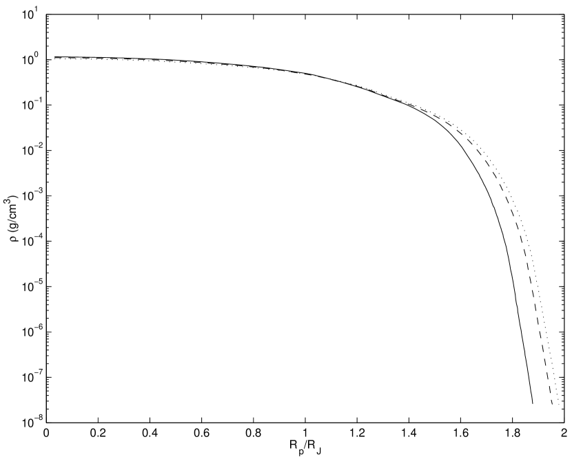
Figure 5: The density profiles of a giant planet in the cases of Model 1 & 6 (dotted curve), Model 2 (solid curve), and Model 5 (dashed curve). Model 1 is a case of uniform heating, while model 6 is a case with the same integrated heating rate but with the energy deposition concentrated in a shell at mass fraction $m_{0}/M_{p}=0.05$. Models 2 and 5 also have the same heating rate but the energy is deposited in shells of mass fraction $m_{0}/M_{p}=0.9999$ and 0.70, respectively.

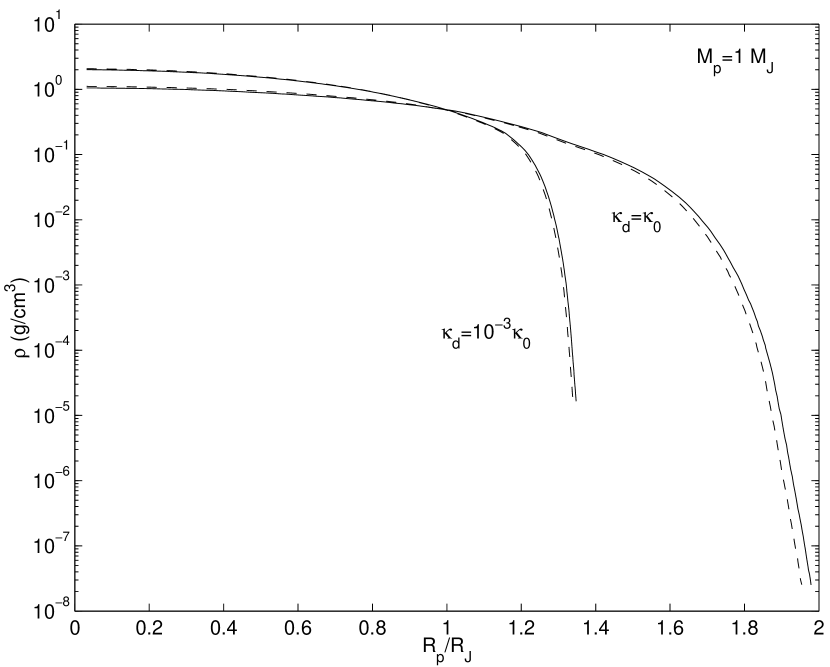
Figure 8: The comparison of the density profiles for the regular grain opacity $\kappa_{d}=\kappa_{0}$ (the solid curve for Model 1 and the dashed curve for Model 4) and for the reduced grain opacity $\kappa_{d}=10^{-3}\kappa_{0}$ (the solid curve for Model 13 and the dashed curve for Model 14). While the heating is deposited uniformly in mass in Models 1 and 13, Model 4 and 14 have the same integrated heating rate but with the energy deposition concentrated in a shell at mass fraction $m_{0}/M_{p}=0.9$.

References

- Alexander & Ferguson (1994) Alexander, D. R., & Ferguson, J. W. 1994, ApJ, 437, 879
- Bodenheimer et al. (2000) Bodenheimer, P. H., Hubickyj, O., & Lissauer, J. J. 2000, Icarus, 143, 2
- Bodenheimer, Laughlin, & Lin (2003) Bodenheimer, P. H., Laughlin, G., & Lin, D. N. C. 2003, ApJ, 592, 555