Strong Gravitational Lensing and Dynamical Dark Energy

Abstract

We study the strong gravitational lensing properties of galaxy clusters obtained from N-body simulations with different kind of Dark Energy (DE). We consider both dynamical DE, due to a scalar field self–interacting through Ratra–Peebles (RP) or SUGRA potentials, and DE with constant negative $w=p/\rho=-1$ (ΛCDM). We have 12 high resolution lensing systems for each cosmological model with a mass greater than $5.0\times 10^{14}$$h^{-1}$M_⊙. Using a Ray Shooting technique we make a detailed analysis of the lensing properties of these clusters with particular attention to the number of arcs and their properties (magnification, length and width). We found that the number of giant arcs produced by galaxy clusters changes in a considerable way from ΛCDM  models to Dynamical Dark Energy models with a RP or SUGRA potentials. These differences originate from the different epochs of cluster formation and from the non-linearity of the strong lensing effect. We suggest the Strong lensing is one of the best tool to discriminate among different kind of Dark Energy.

1 Introduction

The mounting observational evidence for the existence of Dark Energy (DE), which probably accounts for $\sim 70\%$ of the critical density of the Universe [Perlmutter et al. (1999), Riess et al. (1998), Tegmark, Zaldarriaga, & Hamilton(2001), Netterfield et al. (2002), Pogosian, Bond, & Contaldi (2003), Efstathiou et al.(2002), Percival et al. (2002), Spergel et al (2003)], rises a number of questions concerning galaxy formation. The nature of DE is suitably described by the parameter $w=p/\rho$, which characterizes its equation of state. The ΛCDM model ($w=-1$) was extensively studied during the last decade. Recently much more attention was given to physically motivated models with variable $w$ [Mainini, Macciò, & Bonometto (2003a)], for which a number of N–body simulations have been performed (Klypin et al 2003, KMMB03 hereafter, Dolag et al. 2003, Linder & Jenkins 2003, Macciò et al. 2004). One of the main results of KMMB03 was that dynamical DE halos are denser than those with the standard ΛCDM  one. In this work we want to analyze the impact of this higher concentration on the strong lensing properties of the cluster size halos.

Was first noted by Bartelmann et al. (1998) (for OCDM, SCDM and ΛCDM  cosmology) that the predicted number of giant arcs varies by orders of magnitude among different cosmological models. The agreement between data and ΛCDM  simulation was tested by many authors (see Meneghetti et al 2000, Dalal et al. 2003, Wambsganss et al. 2004) but the situation is still unclear. A direct comparison of arcs statistic with observational data is out of the scope of this work, what we want to point out is the capability of Strong Lensing to discriminate between different kinds of Dark Energy (a similar paper but for a different choice of the dynamical DE parameters was recently submitted by Meneghetti et al. (2004)).

Here, using a Ray Shooting technique, we make a lensing analysis of dark matter halos extracted from N-body simulations of cosmological models with varying $w$ arising from physically motivated potentials which admit tracker solutions. In particular, we focus on the two most popular variants of dynamical DE [Wetterich (1988), Ratra & Peebles (1988), Wetterich (1995)]. The first model was proposed by Ratra & Peebles (1984, RP hereafter) and it yields a rather slow evolution of $w$. The second model [Brax & Martin (1999), Brax, Martin, & Riazuelo (2000), Brax & Martin (2000)] is based on potentials found in supergravity (SUGRA) and it results in a much faster evolving $w$. Hence, RP and SUGRA potentials cover a large spectrum of evolving $w$. These potentials are written as

$$V(\phi) = \frac{\Lambda^{4+\alpha}}{\phi^{\alpha}}\qquad RP,$$ (1)

$$V(\phi) = \frac{\Lambda^{4+\alpha}}{\phi^{\alpha}}\exp(4\pi G\phi^{2})~{}~{}~{}SUGRA.$$ (2)

Here $\Lambda$ is an energy scale, currently set in the range $10^{2}$–$10^{10}\,$GeV, relevant for the physics of fundamental interactions. The potentials depend also on the exponent $\alpha$. The parameters $\Lambda$ and $\alpha$ define the DE density parameter $\Omega_{DE}$. However, we prefer to use $\Lambda$ and $\Omega_{DE}$ as independent parameters. Figure 10 in Mainini et al. (2003b) gives examples of $w$ evolution for RP and SUGRA models.

The SUGRA model considered in this paper has $\Lambda=10^{3}$ GeV this implies $w=-0.85$ at $z=0$, but $w$ drastically changes with redshift: $w\approx-0.4$ at $z=5$. The first RP model (RP₁) has the same value for $\Lambda$ of the SUGRA model. At redshift $z=0$ it has $w=-0.5$; then value of $w$ gradually changes with the redshift: at $z=5$ it is close to $-0.4$. Although the $w$ interval spanned by this RP model covers values significantly above -0.8 (not favored by observations), this case is still important both as a limiting reference case and to emphasize that models with constant $w$ and models with variable $w$ produce different results even if average values of $w$ are not so different. For the second RP model (RP₂) we have chosen $\Lambda=10^{-8}$ GeV, in this case the value of the state parameter at redshift $z=0$ is the same of SUGRA: $w(z=0,\Lambda=10^{-8}$ GeV$)=-0.85$. This model is certainly better in agreement with CMB constrains but it loses most of its interest from a theoretical point of view: such a small value of $\Lambda$ has not any clear connection with the physics of fundamental interactions and so it has exactly the same “fine tuning” problem of the ΛCDM  model.

We have normalized all the models in order to have today the same value of the $rms$ density fluctuation on a scale of 8 $h^{-1}$Mpc , that has been chosen as $\sigma_{8}=0.8$.

2 N-body Simulations

The Adaptive Refinement Tree code (ART; Kravtsov, Klypin & Khokhlov 1997) was used to run the simulations. The ART code starts with a uniform grid, which covers the whole computational box. This grid defines the lowest (zeroth) level of resolution of the simulation. The standard Particles-Mesh algorithms are used to compute density and gravitational potential on the zeroth-level mesh. The ART code reaches high force resolution by refining all high density regions using an automated refinement algorithm. The refinements are recursive: the refined regions can also be refined, each subsequent refinement having half of the previous level’s cell size. This creates a hierarchy of refinement meshes of different resolution, size, and geometry covering regions of interest. Because each individual cubic cell can be refined, the shape of the refinement mesh can be arbitrary and match effectively the geometry of the region of interest.

The criterion for refinement is the local density of particles: if the number of particles in a mesh cell (as estimated by the Cloud-In-Cell method) exceeds the level $n_{\rm thresh}$, the cell is split (“refined”) into 8 cells of the next refinement level. The refinement threshold depends on the refinement level. For the zero’s level it is $n_{\rm thresh}=2$. For the higher levels it is set to $n_{\rm thresh}=4$. The code uses the expansion parameter $a$ as the time variable. During the integration, spatial refinement is accompanied by temporal refinement. Namely, each level of refinement, $l$, is integrated with its own time step $\Delta a_{l}=\Delta a_{0}/2^{l}$, where $\Delta a_{0}=3\times 10^{-3}$ is the global time step of the zeroth refinement level. This variable time stepping is very important for accuracy of the results. As the force resolution increases, more steps are needed to integrate the trajectories accurately. Extensive tests of the code and comparisons with other numerical $N$-body codes can be found in Kravtsov (1999) and Knebe et al. (2000). The code was modified to handle DE of different types (Mainini et al 2003b & KMMB03).

We performed a low resolution simulation for each model with the following parameters: box size: 320 $h^{-1}$Mpc, number of particles: $128^{3}$, force resolution: 9.2 $h^{-1}$kpc, all the simulations have the same initial random seed so at $z=0$ the clusters are more or less in the same positions. Than we selected the four massive clusters in the ΛCDM  simulation and re-run them with a mass resolution 64 times higher. The same clusters are also re-run with the same resolution also in the RP and SUGRA models. At the end we have 12 lensing systems (each cluster can be seen by three different orthogonal directions) for each cosmological model, with a mass resolution of $2.03\times 10^{10}\mbox{$h^{-1}$M${}_{\odot}$}$ and a force resolution of 4.8 $h^{-1}$kpc. A complete list of simulation parameters is contained in table 1.

Model	$\Lambda$	Box	Np	Mres.	Fres.
	(GeV)	($h^{-1}$Mpc)		($h^{-1}$M⊙)	($h^{-1}$kpc)
RP1	103	320	5123	$2.03\times 10^{10}$	4.8
RP2	10-8	320	5123	$2.03\times 10^{10}$	4.8
SUGRA	103	320	5123	$2.03\times 10^{10}$	4.8
ΛCDM	0	320	5123	$2.03\times 10^{10}$	4.8

Table 1: Parameters of simulations

3 Lensing Simulations

In order to compute arc statistics for the models discussed above, we adopted a technique similar to the one originally proposed by Bartelmann & Weiss (1994). We center the cluster in a cube of 4 $h^{-1}$Mpc side length and study three lenses, obtained by projecting the particle positions along the coordinate axes. This grants us a total of 12 lens planes per model that we treat as though being due to independent clusters, for our present purposes.

We then divide the projected density field $\Sigma$ by the critical surface mass density for lensing

$$\Sigma_{cr}={c^{2}\over{4\pi G}}{D_{S}\over{D_{L}D_{LS}}}~{},$$ (3)

so obtaining the convergence $k$. Here $c$ is the speed of light, $G$ is the gravitational constant, while $D_{L}$, $D_{S}$, $D_{LS}$ are the angular-diameter distances between lens and observer, source and observer, lens and source, respectively. Once we set the lens and source redshift, the value of the angular diameter distance depends on the cosmological model. We detail this point in the next section. In Figure 1 we show the convergence map for one of the cluster, whose length scale size is 4 $h^{-1}$Mpc. The deflection angle due to this 2D particle distribution, on a given point $\vec{x}$ on the lens plane reads:

$$\vec{\alpha}(\vec{x})=\sum_{j=1}^{N}{{4G}\over{c^{2}}}{{m_{j}}\over{|\vec{x}-\vec{y}_{j}|}}~{}.$$ (4)

Here $\vec{y}_{j}$ is the position of the $j$-th particles and $N$ is the total number of particles.

As direct summation requires a long time, we sped up the code by using a P³M–like algorithm: the lens plane was divided into 128$\times$128 cells and direct summation was applied to particles belonging to the same cell of $\vec{x}$ and for its 8 neighbor cells. Particles in other cells were then seen as a single particle in the cell baricenter, given the total mass of the particles inside the cell.

The deflection angle diverges when the distance between a light ray and a particle is zero. To avoid this unwanted feature we introduce a softening parameter $\epsilon$ in eq:(4); the value $\epsilon$ is tuned on the resolution of the current simulation.

We start to compute $\vec{\alpha}(\vec{x})$ on a regular grid of 256$\times$256 test rays that covered the central quarter of the lens plane, then we propagate a bundle of 2048$\times$2048 light rays and determine the deflection angle on each light ray by bicubic interpolation amongst the four nearest test rays (see section 3.2 for further discussion on the effects of the adopted resolution in the lens mapping).

The relation between images and sources position is given by the lens equation:

$$\vec{y}=\vec{x}-\vec{\alpha}(\vec{x})$$ (5)

and the local properties of the lens mapping are then described by the Jacobian matrix of the lens equation,

$$A_{hk}(\vec{x})={{\partial y_{h}}\over{\partial x_{k}}}=\delta_{hk}-{{\partial\alpha_{h}\over\partial x_{k}}}$$ (6)

The shear components $\gamma_{1}$ and $\gamma_{2}$ are found from $A_{hk}$ through the standard relations:

$$\gamma_{1}(\vec{x})=-{1\over 2}[A_{11}(\vec{x})-A_{22}(\vec{x})],$$ (7)

$$\gamma_{2}(\vec{x})=-{1\over 2}[A_{12}(\vec{x})+A_{21}(\vec{x})],$$ (8)

and the magnifications factor $\mu$ is given by the Jacobian determinant,

$$\mu(\vec{x})={1\over{\det A}}=[A_{11}(\vec{x})A_{22}(\vec{x})-A_{12}(\vec{x})A_{21}(\vec{x})]^{-1}.$$ (9)

Finally, the Jacobian determines the location of the critical curves $\vec{x}_{c}$ on the lens plane, which are defined by $\det A(\vec{x}_{c})=0$. Because of the finite grid resolution, we can only approximately locate them by looking for pairs of adjacent cells with opposite signs of $\det A$. Then, the lens equations

$$\vec{y}_{c}=\vec{x}_{c}-\vec{\alpha}(\vec{x}_{c}),$$ (10)

yield the corresponding caustics $\vec{y}_{c}$, on the source plane.

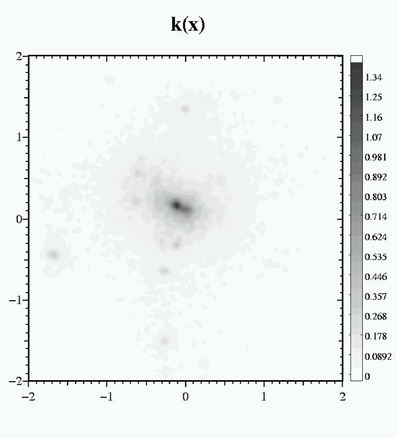
Figure 1: Convergence map for one of the ΛCDM  clusters. The side length is 4 $h^{-1}$Mpc.

3.1 Sources deformation

For statistical purposes one has to distribute and map a large number of sources. We are interested in arc properties and arcs form near caustics; so for numerical efficiency we have to distribute less sources in those part of the source plane that are far away from any caustics, and more sources close or inside the caustics. We follow the method introduced by Miralda-Escudè (1993) and later adapted to non-analytical models by Bartelmann & Weiss (1994). In the previous section we have obtained the deflection angles for the $\vec{x}_{ij}$ (with i,j=1,…,2048) positions on the lens (or image) plane, using the lens equation (10) we can obtain the corresponding positions on the source plane $\vec{y}_{ij}(\vec{x}_{ij})$, as usual we call this discrete transformation the mapping table.

We model elliptical sources with axial ratios randomly drawn from the interval $[0.5;1]$ and area equal to that of a circle with radius $r_{s}=0.5^{\prime\prime}$. We first distribute sources on a coarse grid of 32x32, defined in the central quarter of the source plane covered by the light rays traced (due to convergence only a restricted part of the source plane can be reached by the light rays traced from the observer through the lens plane). From the mapping table we have obtained the magnification ($\mu$), if it changes by more than one (absolute value) between two sources, we place an additional source between both, in this way we increase the resolution by a factor 2 in each dimension. For the n-th iteration of source positions the criterium to add additional sources is that magnification changes by $2^{n-1}$. We repeat this procedure four times to obtain the final list of source positions. To compensate for this artificial increase in the source number density we assign a statistical weight of $2^{1-n}$ to each image of a source placed during the $n$-th grid refinement. On average we have about 15000 sources for each lensing system.

3.2 Arcs Analysis

To find the images of an extended source, all images-plane positions $\vec{x}$ are checked if the corresponding entry in the map table $\vec{y}$ lies within the source: i.e. for an elliptical source with axes $a,b$ and centered in $(y^{c}_{1};y^{c}_{2})$ it is checked if:

$${{(y_{1}-y_{1}^{c})^{2}}\over a^{2}}+{{(y_{2}-y_{2}^{c})^{2}}\over b^{2}}\leq 1,$$ (11)

where $(y_{1},y_{2})$ are the components of the vector $\vec{y}$.

Those points fulfilling the previous equation are part of one of the source images and are called image points. We then use a standard friends-of-friends algorithm to group together image points within connected regions, since they belong to the same image (the number of images of one source ranges from 1 to 5 for our clusters).

We measure arc properties using a method based on Bartelmann & Weiss (1994). The arc area and magnification are found by summing the areas of the pixel falling into the image. Arc lengths are estimated by first finding the arc center, then finding the arc pixel farest from the centroid as well as the pixel farest from this pixel. The arc length is then given by the sum of the lengths of the two lines connecting these three points. The arc width is defined as the ratio between the arc area and the arc length.

In Figure 2 we plot the relation between length/width ratio and magnification; we found a good agreement with previous results obtained by Dalal et al. (2003). The scatter in this relation is due to local fluctuations in the surface mass density, highly distorted images are also highly magnified, but the converse is not always true.

Figure 2: Magnification vs. length/width ratio for ΛCDM  clusters. These two quantities are equal for an isothermal sphere lens.

Before proceeding with our analysis we have performed some tests on the resolution adopted in our ray shooting code; figure 3 shows the fraction of sources (number of sources divided by the total number) vs. their length/width for different values of the resolution of the lens mapping grid $N_{hr}^{2}$ (results are for the ΛCDM model with $z_{l}=0.3$ and $z_{s}=1.0$). If the resolution of the lens mapping is not high enough the critical curves are too small compared to the source size and a spurious cut off in the number of arcs with $L/W>10$ appears. This cut off is totally artificial and it vanishes for $N_{hr}\geq 2048$. As figure 3 shows the results are stable also for a higher value of $N_{hr}$ (4096), then in order to have a good compromise between resolution and computational time we have adopted $N_{hr}=2048$ in the following.

Figure 3: Fraction of sources mapped in an arc vs length/width ratio of the arc for different values of the resolution of the lensing mapping. All curves are for the ΛCDM  model with $z_{l}=1.0$ and $z_{s}=0.3$.

4 Arcs Statistics

In this paper we aim to compare the lensing properties of a given cluster as it appears in different cosmological models. There are three main features that affect the number of giant arcs: the concentration of the halo, the total number of lensing systems at a given redshift and the value of the critical surface mass density ($\Sigma_{cr}$).

As predicted analytically by Bartelmann et al (2002) (for constant $w$ models) and first noted in numerical Nbody simulations by KMMB03, and then confirmed by Dolag et al (2003) and Linder & Jenkins (2003), the concentration of dynamical DE halos is greater than the concentration of ΛCDM  ones. Here we use the same definition of concentration of KMMB03: the ratio of the radius at the overdensity of the ΛCDM  model (103 times the critical density) to the characteristic (“core”) radius of the NFW profile. (see however KMMB03 for more details). A greater concentration increases the probability of forming giant arcs. In Figure 4 we report the density profile of the same halo simulated in different cosmological models. The RP₁ halo is clearly denser and more concentrated than the ΛCDM  halo with the SUGRA halo laying in between; the RP₂ halo (which is not shown in this plot) has a concentration parameter close to the one of the ΛCDM  model.

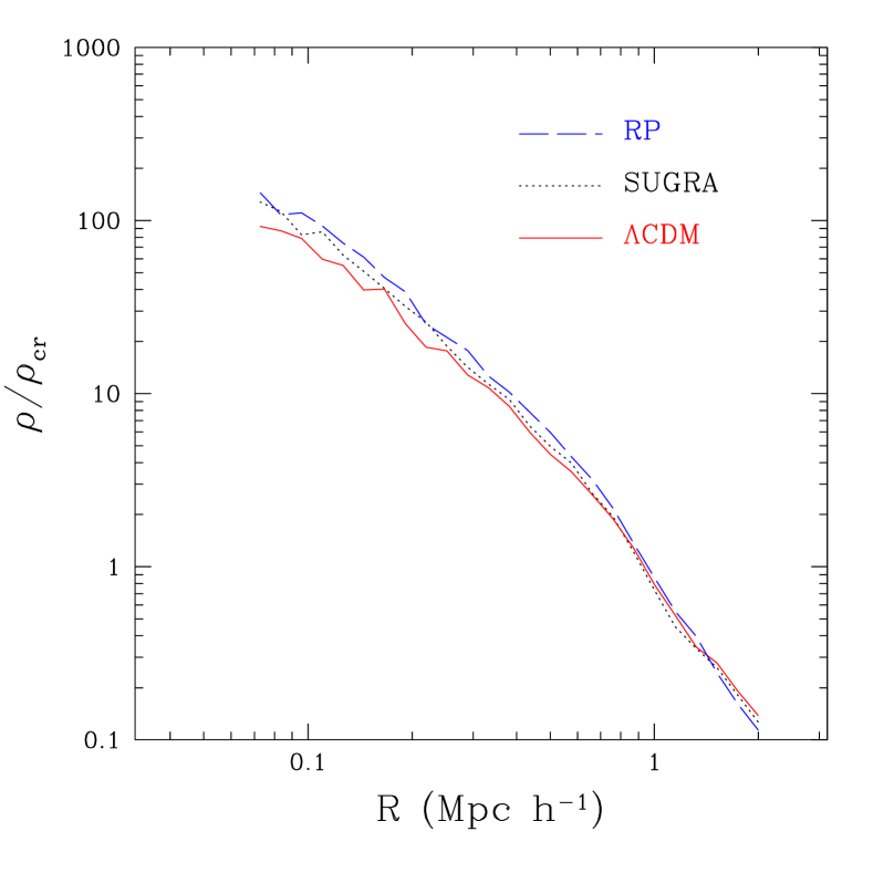
Figure 4: Density profile of the same halo simulated in different model. The red curve is for ΛCDM , the black one for SUGRA and the blue for RP₁. The halo has a virial mass of $6\times 10^{14}\mbox{$h^{-1}$M${}_{\odot}$}~{}$.

The expected number of objects with a mass exceeding $4\times 10^{14}\mbox{$h^{-1}$M${}_{\odot}$}$ (in order to produce multiple images) at a given redshift (in this case $z=0.4$) can be estimated using a Press & Schechter formalism (see Mainini et al 2003a). In dynamical DE, objects form earlier than in ΛCDM, so we have more lensing systems per Mpc³ at $z=0.3$. This can be taken into account by multiplying the number of arcs by 1.3, 1.21 and 1.12 in RP₁, SUGRA and RP₂ respectively. (In Figure 5 we report the evolution with redshift of the mass function for a mass threshold of $4.0\times 10^{14}\mbox{$h^{-1}$M${}_{\odot}$}$).

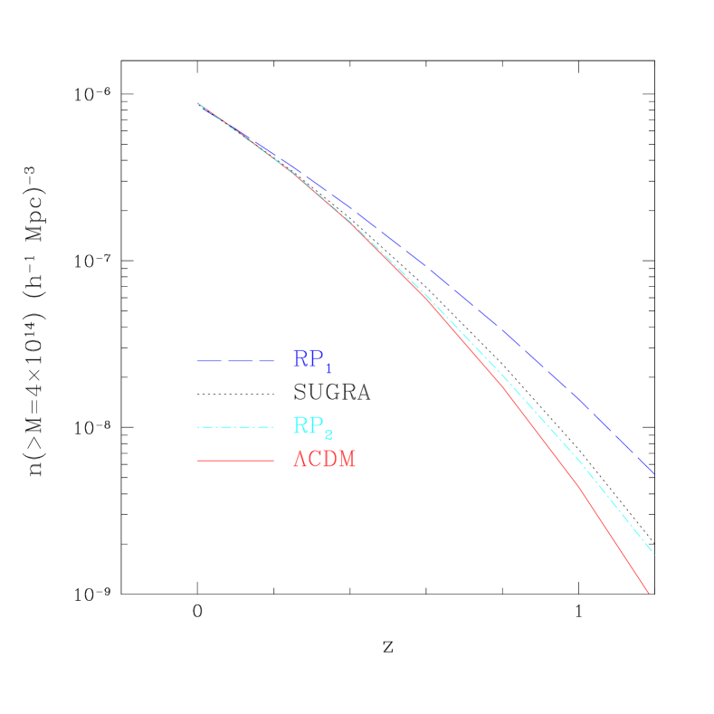
Figure 5: Number density of halos with a mass greater than $4.0\times 10^{14}\mbox{$h^{-1}$M${}_{\odot}$}$ for ΛCDM  (low solid curve), SUGRA (dotted curve) and the two RP models. The value of $\Lambda$ is $10^{3}$ GeV for both RP₁ and SUGRA and $10^{-8}$ GeV for RP₂.

The evolution of the scale factor $a$ with time also depends on the model. This implies that, at a given redshift $z=1/a-1$, the angular diameter distance $D_{ad}$ is model dependent; in fact its value is given by:

$$D_{ad}(a)={ac\over{H_{0}}}\int_{a}^{1}\sqrt{{a(1-\Omega_{DE}(a))}\over{\Omega_{m,0}}}~{}~{}\rm{d}a~{}.$$ (12)

Here $c$ is the speed of light, $H_{0}$ and $\Omega_{m,0}$ are the present value of the Hubble constant and the matter density parameter and $\Omega_{DE}(a)$ gives the evolution of the DE density parameter with the expansion factor. To compute $\Omega_{DE}(a)$ for RP and SUGRA models we have used the analytical expression of Mainini et al (2003b). In Figure 6 we show the value of the critical surface mass density for the adopted cosmological models. The different values for $\Sigma_{cr}$ mean that a ΛCDM  halo yields more arcs than a dynamical DE halo, if they have the same surface mass density. The effect of the different values of the angular diameter distance tends therefore to reduce the number of arcs in dynamical DE models.

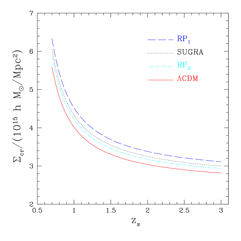
Figure 6: Value of the critical surface mass density $\Sigma_{cr}$ in different cosmological models, for all the curves we choose a lens redshift $z_{L}=0.4$

The first result of our analysis is shown in Figure 7, where we plot the fraction of sources (number of sources divided by the total number) vs. their length/width ratio for a cluster (lens) redshift $z_{l}=0.3$, where lensing is most efficient for a source redshift of 1.0 (as shown later in figure 11). As expected, the RP₁ model produces more distorted images, due to its more concentrated halos. The SUGRA and RP₂ models are quite similar for $L/W>10$ and they lay in between RP₁ and ΛCDM  which, as expected, produces less highly distorted images than the dynamical DE models. We want to underline that part of the higher lensing signal due to the higher concentration of dark matter halos in such models is canceled by the increased $\Sigma_{cr}$ value. This effect is clearly illustrated in figure 8 where we have computed the arc statistics in a SUGRA model using the ΛCDM  critical surface density. As expected, we have obtained a result for SUGRA that is closer to the RP₁ one.

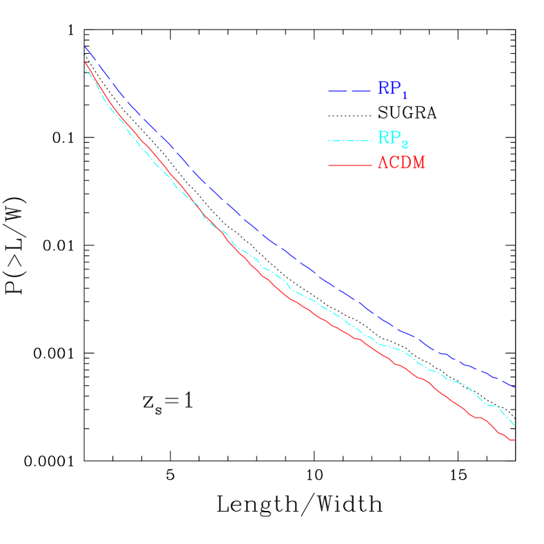
Figure 7: Fraction of sources mapped in an arc vs length/width ratio of the arc. Upper curve is RP₁ (blue) than from top to bottom we have SUGRA (red), RP₂ (cyan) and ΛCDM  (black) results.

Figure 8: Same plot of Figure 7 for the SUGRA model where the arc properties are computed using $\Sigma_{cr}({\char 3\relax CDM}~{})$ (solid line) and $\Sigma_{cr}(SUGRA)$ (dashed line).

As pointed out by many authors (Wambsganss et al. 2003, Dalal et al. 2003) the number of arcs that a cluster is able to produce is strongly related to the redshift of the sources (although the strength of this effect is not yet completely understood, different authors found different results). In Figure 9 we plot the arc number counts for the ΛCDM  model for $z_{s}=1$ (dashed line) and $z_{s}=2$ (solid line). As in previous work we found that the number of arcs increases if we increase the source redshifts. Figure 10 shows the same results of Figure 7 but for $z_{s}=2$.

As expected, the total number of arcs increases in all cosmological models. Again we have a sort of hierarchy of results according to what is expected from the dynamical evolution of dark matter halos in the corresponding cosmological model.

Moreover, due to the lower difference in the value of $\Sigma_{cr}$ for this sources redshift, the four models are better separated, expecially the SUGRA and RP₂ ones. A difference between these two models is somewhat expected even if they have the same value of state parameter today ($w=-0.84$), this arises from the different evolution of $w$: in SUGRA it drastically changes with redshift ($w=-0.4$ at $z=5$) when it is more constant in RP₂ ($w=-0.72$ at $z=5$).

Figure 9: Arcs counts for two different values of the sources redshift in the ΛCDM  model.

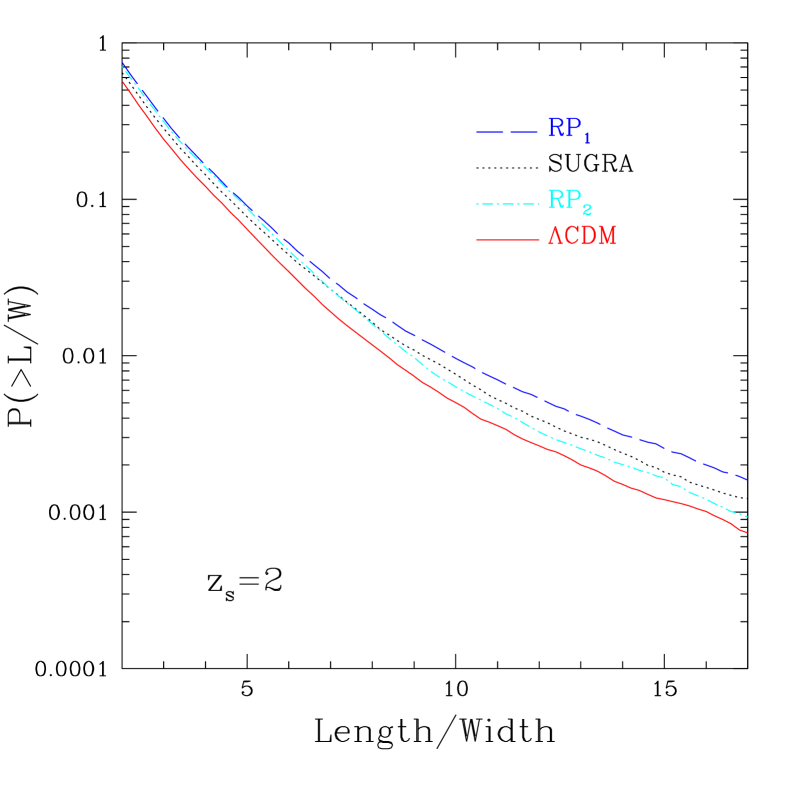
Figure 10: The same of Figure 7 for $z_{s}=2$. With this value for the source redshift the number of arcs increases in all the models.

As final result in figure 11 we show the evolution with the lens redshift of the number of arcs for two different choices of the length/width ration: 10 and 7.5 (the redshift of the sources is $z_{s}=1.0$). On average the the RP₁ model is always above the others, instead the different between SUGRA and ΛCDM  is more or less constant at all redshift and the lensing signal decreases rapidly for $z>0.45$.

The RP₂ model has a sort of double behavior: it is close to ΛCDM  for $z>0.35$ but it is more similar to SUGRA for $z<0.35$, we think that this bimodality is due again to the evolution of the state parameter in this model expecially if compared to the SUGRA one: the ration $w_{RP_{2}}/w_{SU}$ decreases with redshift towards unity at $z=0$, so it is less different from ΛCDM  at high redshift in respect to SUGRA.

The peaks in the lensing signal have slightly different positions in the different models. As argued by other authors (Torri et al 2004, Meneghetti et al. 2005) this could be due to time offset between merger events in different dark energy cosmologies.

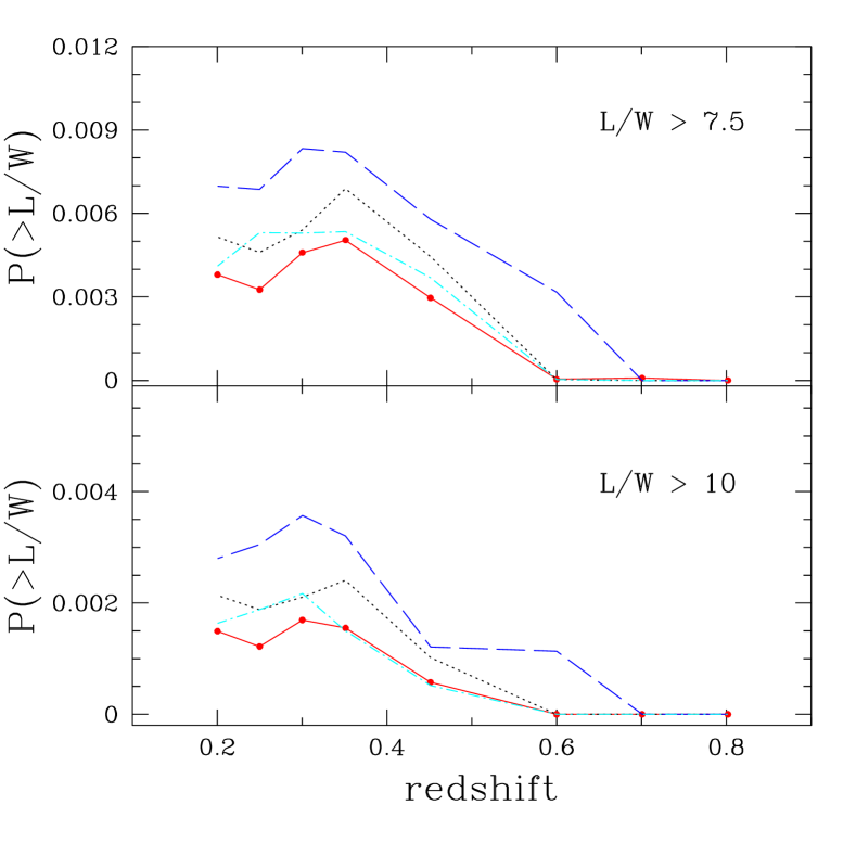
Figure 11: Number of arcs vs the lens redshift for two different thresholds of the $L/W$ ratio: 10 and 7.5. Solid line is for ΛCDM , dashed for RP₁, dot-dashed for RP₂ and dotted for SUGRA ($z_{s}=1.0$).

5 Discussion and conclusions

Models with dynamical DE are in an infant state. We do not know the nature of DE. Thus, the state parameter $w(t)$ is still uncertain. In view of this functional indetermination, at first sight, it could seem that the situation is hopeless.

In spite of that, we can outline some general trends that result from our analysis: in dynamical DE models, halos tend to collapse earlier than in a ΛCDM  model with the same normalization at $z=0$. As the result, halos are more concentrated and denser in their inner parts (KMMB03). Starting from this finding we have explored the consequences of this higher concentration, on strong lensing properties of dark matter halos, in SUGRA and RP cosmologies.

We found that RP₁ halos (obtained assuming the cluster abundance of the power spectrum and a value for the energy scale $\Lambda$ in the range suggested by the physics of fundamental interactions) produce a higher number of arcs with a $L/W>10$ if compared to the standard ΛCDM  model. This model (RP₁) is marginal consistent with observations and its purpose is mainly to illustrate the principal effect of a dynamical dark energy component on arcs statistic.

The second model we analyzed based on RP potential (RP₂) is more realistic from an observational point of view but less motivated by theoretical arguments. This model produce about 50% more arcs with $L/W>10$ than the ΛCDM  one for $z_{l}=0.3$ and $z_{s}=1$ but it is marginally distinguishable from ΛCDM  for lensing system at moderate high redshift ($z_{l}>0.35$, fig 11) or for high redshift sources/arcs ($z_{l}=0.3$ and $z_{s}=2$).

The SUGRA model is always in between the ΛCDM  and the RP₁ models and it produces about 70-80% more arcs than ΛCDM . This difference is almost constant both changing the sources and the lens redshift and it tends to disappear for $z_{l}>0.6$ (for $z_{s}=1.0$) where all the lensing systems considered in this paper ($M_{l}\approx 5\times 10^{14}$ ) are unable to produce highly distorted images (except in the test model RP₁). We also noted that part of the stronger lensing signal due to the higher concentration of halos in dynamical DE models is partially canceled by geometrical effects that increase the critical surface density in such models (fig. 6 and fig. 8).

As final remark we would like to stress that arc statistic is a powerful tool to investigate the nature of the Dark Energy. The forthcoming observational surveys(i.e. CFHT Legacy Survey, SDSS and others) will improve the statistic of giant arcs on the sky (for example the RCS-2 Survey (Gladders et al. 2003) will cover an area of 830 deg² and is expected to produce 50-100 new arcs). Such an observational material will provide a discrimination between DE cosmologies possibly allowing to constrain the $\Lambda$ scale of the SUGRA and RP potentials.

References

- [Bartelmann et al (1998)] Bartelmann M., Huss A., Carlberg J., Jenkins A. & Pearce F. 1998, A&A 330, 1
- [Bartelmann & Weiss (1994)] Bartelmann M. & Weiss, A. 1994, A&A 287, 1
- [Bartelmann et al (2002)] Bartelmann M., Perrotta F. & Baccigalupi C. 2002, A&A 396, 21
- [Bartelmann et al (2003)] Bartelmann M., Meneghetti, M., Perrotta F., Baccigalupi C. & Moschardini, L. 2003, A&A 409, 449B
- [Brax & Martin (1999)] Brax, P. & Martin, J., 1999, Phys.Lett., B468, 40
- [Brax & Martin (2000)] Brax, P. & Martin, J., 2000, Phys.Rev. D, 61, 103502
- [Brax, Martin, & Riazuelo (2000)] Brax P., Martin J. & Riazuelo A., 2000, Phys.Rev. D, 62, 103505
- [Dalal et al.(2003)] Dalal, N., Holder, G. & Hennawi, J.F. 2003, astro-ph/0310306
- [Dolag et al. 2003] Dolag, K, Bartelmann M., Perrotta F., Baccigalupi C., Moschardini, L., Meneghetti, M. & Tormen, G. 2003, astro-ph/0309771
- [Efstathiou et al.(2002)] Efstathiou, G. et al., 2002, MNRAS, 330, 29
- [Flores et al.(2000)] Flores, R.A., Maller, A.H. & Primack, J.R. 2000, ApJ, 535, 555
- [Gladders et al (2003)] Gladders, M.D., Hoekstra, H., Yee, H.K.C., Hall, P.B. & Barrientos, L.F. 2003, ApJ, 593, 48
- [Klypin et al. (2003b)] Klypin, A., Macciò A.V., Mainini R. & Bonometto S.A., 2003, ApJ, 599, 31
- [Knebe et al. (2000)] Knebe, A., Kravtsov A., Gottlober, S. & Klypin A. 2000, MNRAS, 317, 630
- [Kravtsov, Klypin, & Khokhlov (1997)] Kravtsov A., Klypin A. & Khokhlov A., 1997 ApJ, 111, 73 K
- [Le Fevre et al. (1994)] Le Fevre et al. 1994, ApJ, 422, L5
- [Linder, & Jenkins (2003)] Linder E., & Jenkins A., 2003, MNRAS, 346, 573
- [Luppino et al. (1999)] Luppino, G.A., Gioia, I.M., Hammer, F., Le Fevre, O. & Annis, J.A. 1999, A&AS,136, 117
- [Macciò et al (2004)] Macciò A.V., Quercellini, C., Mainini R., Amendola, L. & Bonometto S.A., 2004, Phys.Rev. D, 69, 123516
- [Mainini, Macciò, & Bonometto (2003a)] Mainini R., Macciò A.V. & Bonometto S.A., 2003a, NewA 8, 172
- [Mainini et al. (2003b)] Mainini R., Macciò A.V., Bonometto S.A., & Klypin, A., 2003b, ApJ, 599, 24
- [Meneghetti et al (2003)] Meneghetti M., Bartelmann M. & Moscardini L. 2003, MNRAS 346, 67
- [Meneghetti et al (2000)] Meneghetti M., Bolzonella M., Bartelmann M., Moscardini L. & Tormen G. 2000, MNRAS 314, 338M
- [Meneghetti et al. 2004] Meneghetti, M., Bartelmann M., Dolag, K., Moschardini, L., Perrotta F., Baccigalupi C., & Tormen, G. 2003, astro-ph/0405070
- [Miralda-Escudè] Miralda-Escudè J. 1993, ApJ, 403, 497
- [Netterfield et al. (2002)] Netterfield, C. B. et al. 2002, ApJ, 571, 604
- [Percival et al. (2002)] Percival W.J. et al., 2002, MNRAS, 337, 1068
- [Perlmutter et al. (1999)] Perlmutter S. et al., 1999, ApJ, 517, 565
- [Pogosian, Bond, & Contaldi (2003)] Pogosian, D., Bond, J.R., & Contaldi, C. 2003, astro-ph/0301310
- [Ratra & Peebles (1988)] Ratra B., Peebles P.J.E., 1988, Phys.Rev.D, 37, 3406
- [Riess et al. (1998)] Riess, A.G. et al., 1998, AJ, 116, 1009
- [Spergel et al (2003)] Spergel et al. 2003, astro–ph/0302209
- [Tegmark, Zaldarriaga, & Hamilton(2001)] Tegmark, M., Zaldarriaga, M., & Hamilton, A. J. 2001, Phys. Rev. D, 63, 43007
- [Torri et al. (2004)] Torri, E., Meneghetti, M., Bartelamann, M., Moscardini, L., Rasia, E. & Tormen, G., 2004, MNRAS 349, 476
- [Wambsganss et al (2003)] Wambsganss, J., Bode, P. & Ostriker, J. P. 2003, astro-ph/0306088
- [Wetterich (1988)] Wetterich C., 1988, Nucl.Phys.B, 302, 668
- [Wetterich (1995)] Wetterich C., 1995 A&A 301, 32