The Temperature of the CMB at 10 GHz

Abstract

We report the results of an effort to measure the low frequency portion of the spectrum of the Cosmic Microwave Background Radiation (CMB), using a balloon-borne instrument called ARCADE (Absolute Radiometer for Cosmology, Astrophysics, and Diffuse Emission). These measurements are to search for deviations from a thermal spectrum that are expected to exist in the CMB due to various processes in the early universe.

The radiometric temperature was measured at 10 and 30 GHz using a cryogenic open-aperture instrument with no emissive windows. An external blackbody calibrator provides an in situ reference. A linear model is used to compare the radiometer output to a set of thermometers on the instrument. The unmodeled residuals are less than 50 mK peak-to-peak with a weighted RMS of 6 mK. Small corrections are made for the residual emission from the flight train, atmosphere, and foreground Galactic emission. The measured radiometric temperature of the CMB is 2.721$\pm.010$ K at 10 GHz and 2.694$\pm 0.032$ K at 30 GHz.

1. INTRODUCTION

Since the discovery of the CMB a key question has been: How does it deviate from a perfect uniform black body spectrum? The FIRAS (Far InfraRed Absolute Spectrophotometer) instrument (Fixsen & Mather 2002, Brodd et al. 1997) has shown the spectrum is nearly an ideal black body spectrum from $\sim 60$ GHz to $\sim 600$ GHz with temperature 2.725$\pm$.001 K. At lower frequencies the spectrum is not so tightly constrained; plausible physical processes (reionization, particle decay) could generate detectable distortions below 10 GHz while remaining undetectable by the FIRAS instrument. The ARCADE (Absolute Radiometer for Cosmology, Astrophysics and Diffuse Emission) experiment observes the CMB spectrum at frequencies a decade below FIRAS to search for potential distortions from a blackbody spectrum.

The frequency spectrum of the cosmic microwave background (CMB) carries a history of energy transfer between the evolving matter and radiation fields in the early universe. Energetic events in the early universe (particle decay, star formation) heat the diffuse matter which then cools via interactions with the background radiation, distorting the radiation spectrum away from a blackbody. The amplitude and shape of the resulting distortion depend on the magnitude and redshift of the energy transfer (Burigana et al. 1991, Burigana et al. 1995).

The primary cooling mechanism is Compton scattering of hot electrons against a colder background of CMB photons, characterized by the dimensionless integral

$$y=\int^{z}_{0}~{}\frac{k[T_{e}(z)-T_{\gamma}(z)]}{m_{e}c^{2}}\sigma_{T}n_{e}(z)c\frac{dt}{dz^{\prime}}dz^{\prime},$$ (1)

of the electron pressure $n_{e}kT_{e}$ along the line of sight, where $m_{e}$, $n_{e}$ and $T_{e}$ are the electron mass, spatial density, and temperature, $T_{\gamma}$ is the photon temperature, $k$ is Boltzmann’s constant, $z$ is redshift, and $\sigma_{T}$ denotes the Thomson cross section (Sunyaev & Zeldovich 1970). For recent energy releases $z<10^{4}$, the gas is optically thin, resulting in a uniform decrement $\Delta T_{\rm RJ}=T_{\gamma}(1-2y)$ in the Rayleigh-Jeans part of the spectrum where there are too few photons, and an exponential rise in temperature in the Wien region with too many photons. The magnitude of the distortion is related to the total energy transfer

$$\frac{\Delta{\rm E}}{\rm E}={\rm e}^{4y}-1\approx 4y$$ (2)

Energy transfer at higher redshift $10^{4}<z<10^{7}$ approaches the equilibrium Bose-Einstein distribution, characterized by the dimensionless chemical potential $\mu_{0}=1.4\frac{\Delta{\rm E}}{\rm E}.$ Free-free emission thermalizes the spectrum at long wavelengths. Including this effect, the chemical potential becomes frequency-dependent,

$$\mu(x)=\mu_{0}\exp(-\frac{2x_{b}}{x}),$$ (3)

where $x_{b}$ is the transition frequency at which Compton scattering of photons to higher frequencies is balanced by free-free creation of new photons. The resulting spectrum has a sharp drop in brightness temperature at centimeter wavelengths (Burigana et al. 1991). A chemical potential distortion would arise, for instance, from the late decay of heavy particles produced at much higher redshifts.

Free-free emission can also be an important cooling mechanism. The distortion to the present-day CMB spectrum is given by

$$\Delta T_{\rm ff}=T_{\gamma}\frac{Y_{\rm ff}}{x^{2}}$$ (4)

where $x$ is the dimensionless frequency $h\nu/kT_{\gamma}$, $Y_{\rm ff}$ is the optical depth to free-free emission

$$Y_{\rm ff}=\int^{z}_{0}~{}\frac{k[T_{e}(z)-T_{\gamma}(z)]}{T_{e}(z)}\frac{8\pi e^{6}h^{2}n_{e}^{2}g}{3m_{e}(kT_{\gamma})^{3}\sqrt{6\pi m_{e}kT_{e}}}\frac{dt}{dz^{\prime}}dz^{\prime},$$ (5)

and g is the Gaunt factor (Bartlett & Stebbins 1991). The distorted CMB spectrum is characterized by a quadratic rise in temperature at long wavelengths. Such a distortion is an expected signal of the reionization of the intergalactic medium by the first collapsed structures.

Figure 1.— Current 95% confidence upper limits to distorted CMB spectra. Measurements at short wavelengths (Fixsen et al. 1996) do not preclude detectable signals at wavelengths longer than 1 cm.

Figure 1 shows current upper limits to CMB spectral distortions. Measurements at wavelengths shorter than 1 cm are consistent with a blackbody spectrum, limiting $y<14\times 10^{-6}$ and $\mu<9\times 10^{-5}$ at 95% confidence (Fixsen et al. 1996, Gush et al. 1990). Direct observational limits at longer wavelengths are weak. Reionization is expected to produce a cosmological free-free background with amplitude of a few mK at frequency 3 GHz (Haiman & Loeb 1997, Oh 1999). The most precise observations (Table 1) have uncertainties much larger than the predicted signal from reionization. Existing data only constrain $|Y_{\rm ff}|~{}<~{}1.9\times 10^{-5}$, corresponding to temperature distortions $\Delta T<19$ mK at 3 GHz (Bersanelli et al. 1994).

Uncertainties in previous measurements have been dominated by systematic uncertainties in the correction for emission from the atmosphere, Galactic foregrounds, or warm parts of the instrument. ARCADE represents a long-term effort to improve measurements at cm wavelengths using a cryogenic balloon-borne instrument designed to minimize these systematic errors. This paper presents the first results from the ARCADE program.

2. THE INSTRUMENT

The ARCADE is a balloon-borne instrument with two radiometers at 10 and 30 GHz mounted in a liquid helium dewar. Each radiometer consists of cryogenic and room temperature components. A corrugated horn antenna, a Dicke switch consisting of a waveguide ferrite latching switch, an internal reference load constructed from a waveguide termination, and GaAs HEMT amplifier comprise the cryogenic components. The signal then passes to a 270 K section consisting of additional amplification and separation into two sub-bands followed by diode detectors, making four channels in all (Kogut et al. 2004a). In addition there is an external calibrator which can be positioned to fully cover the aperture of either the 10 or 30 GHz horn (Kogut et al. 2004b). Helium pumps and heaters allow thermal control of the cryogenic components which are kept at 2-8 K during the critical observations.

To minimize instrumental systematic effects the horns are cooled to approximately the temperature of the CMB (2.7 K). The horns have a $16^{\circ}$ full-width-half-maximum beam and are pointed $30^{\circ}$ from the zenith to minimize acceptance of balloon and flight train emission. A helium cooled flare reduces contamination from ground emission. No windows are used. Air is kept from the instrument by the efflux of helium gas.

Table 1 Previous low frequency CMB measurements and their uncertainties from the literature.

Temperature	uncertainty	frequency	source
K	mK	GHz
2.783	25	25	Johnson & Wilkinson, 1987
2.730	14	10.7	Staggs et al., 1996b
2.64	60	7.5	Levin et al., 1992
2.55	140	2	Bersanelli et al., 1994
2.26	200	1.47	Bersanelli et al., 1995
2.66	320	1.4	Staggs et al., 1996a
3.45	780	1.28	Raghunathan & Subrahmanyan

The Dicke switch chops between the reference and the horn antenna at 100 Hz. Following the HEMT amplifier, outside the dewar, each radiometer has a warm amplifier followed by narrow and wide filters terminated by two detectors. The detectors are followed by lockin amplifiers running synchronously with the Dicke switch. The bandwidths of the 10 GHz narrow and wide and the 30 GHz narrow and wide radiometers are: 0.1, 1.1, 1.0, and 2.9 GHz respectively. The raw sensitivities of these 4 radiometer channels are: 2.3, 0.7, 4.8, and 2.8 mK$\sqrt{{\rm Hz}}$ respectively. The instrument details are discussed by Kogut et al. (2004a).

Other instrumentation on the ARCADE includes a magnetometer and tilt meter to determine the pointing of the radiometers. A GPS receiver collects position and altitude information. Thermometers, voltage and current sensors collect information on the condition of the instrument. A commandable rotator allows rotation of the entire ARCADE gondola at $\sim 0.5$ RPM. A commandable tilt actuator allows tipping of the dewar with the radiometers to measure residual beam and atmospheric effects. A camera provides in flight video pictures of the aperture plane. The camera transmitter interferes with the radiometers so the data taken while the camera is on are not used for science.

The sky temperature estimate depends critically on the measurement of the calibrator temperature. The other components (horn, switch, cold reference, and amplifier) become merely a transfer standard to compare the measurements when looking at the sky to the measurements when looking at the calibrator. The calibrator is addressed by Kogut et al. (2004b) in a companion paper. There are 7 thermometers embedded in the calibrator and its thermal buffer plate: 3 at the tips of the calibrator (T1, T2, T3), 2 at the base of the calibrator (T4, T5) and 2 on the control plate (B1, B2). These ruthenium oxide thermometers (Fixsen et al. 2002) are read out at approximately 1 Hz with .15 mK precision and 2 mK accuracy (both are poorer at temperatuers above 2.7 K). The thermometers have been calibrated on four separate occasions over 5 years with absolute calibrations stable to 2 mK. In addition to the NIST standard thermometer, the lambda transition to superfluid helium at 2.18 K is clearly seen in the calibration data providing an absolute in situ reference.

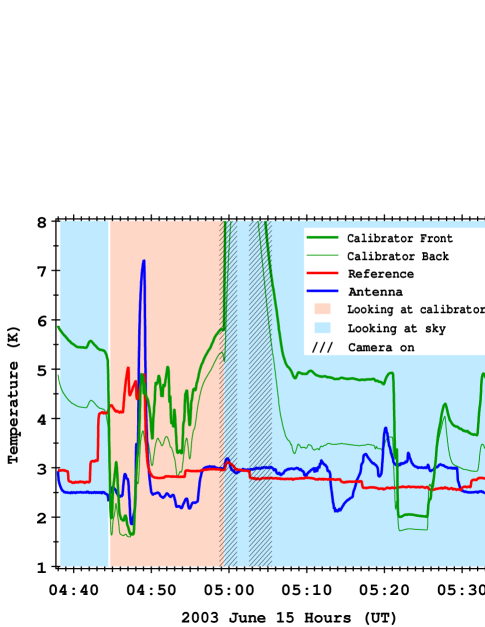
Figure 2.— The temperatures of critical components for the 10 GHz radiometer during the flight. Solid lines indicate component temperatures. Vertical bands indicate whether the 10 GHz antenna viewed the sky or the external calibrator. Cross-hatching shows times when the camera was turned on; data from these times are not used for science analysis.

3. THE OBSERVATIONS

The ARCADE instrument was launched from Palestine TX on a SF3-11.82 balloon 2003 Jun 15 at 1:00 UT after an engineering launch the previous year. At approximately 2:20 UT the instrument reached 21 km so the helium became superfluid. At 2:50 UT the superfluid fountain effect pumps were engaged to cool the upper components of the radiometer and the external calibrator.

The ARCADE reached a float altitude of 35 km at 4:00 UT. The cover protecting the cryogenic components was opened at 4:04 UT. Radiometer gains were adjusted as the external calibrator cooled and were set at their final values at 4:27 UT. The calibrator was moved to the 30 GHz radiometer at 4:32 UT. After some calibration of the 30 GHz radiometer the calibrator was moved to the 10 GHz radiometer at 4:44 UT. The next 10 minutes provide the key 10 GHz calibration data. At 4:54 UT the calibrator was moved to the 30 GHz radiometer. The camera was turned on to verify this move and turned off at 5:00 UT.

A command was sent to move the calibrator back to the 10 GHz radiometer at 5:07 UT and the camera was turned on to verify the move. However, the calibrator motor failed and no further moves of the calibrator were possible. At 5:11 UT the camera was again turned off. At 5:20 UT tipping maneuvers commenced and continued until 5:36 UT.

The helium was exhausted by 7:20 and the ARCADE continued to operate until 8:30 UT but without the ability to move the calibrator only engineering data were collected after 5:36. The most useful observations were from 4:36 UT to 5:36 UT and all of the following derivations will use various subsets of this data. Some of the temperatures for this time are shown in Figure 2.

4. ANTENNA TEMPERATURE ESTIMATION

Conceptually the calibration process is straightforward. The calibrator is placed over the aperture of a radiometer, and the four cryogenic components of the radiometer (horn, Dicke switch, reference, and amplifier) are each warmed and cooled to allow the measurement of the coupling or emission from each component into the radiometer. The calibrator temperature is also changed to measure the responsivity of the radiometer. The calibrator is then moved away so the radiometer observes the sky; the parameters measured while observing the calibrator are used to deduce the antenna temperature of the sky.

The most efficient use of the data uses all of the component temperature variations to obtain the best emissivity estimations, so a general least squares fit is used to solve for all of the emissivities simultaneously. By adding the assumption that the sky is a stable but unknown temperature, the fit can take advantage of the component temperature changes during the sky observations as well. The corrections for instrument and Galactic foreground are included in the least squares solution.

Ideally the temperature of the cryogenic components is near that of the CMB. A linear model can then be used to predict the radiometer output:

$$R=gE\cdot T$$ (6)

where $g$ is the responsivity of the radiometer, $T$ is the matrix of temperatures (each row is a component, each column a time), $E$ is the vector of emissivities and $R$ is a vector of radiometer readings. Since neither $g$ nor $E$ is known a priori, they are combined; $A=gE$. A least squares fit:

$$A=(T\cdot W\cdot T^{T})^{-1}\cdot T^{T}\cdot W\cdot R$$ (7)

produces the weighted solution to the optimum parameterization $A$, where $W$ is a weight matrix.

The list of temperatures in $T$ in the full fit includes: Five RuO thermometers embedded in the absorber of the external calibrator, two thermometers in the external calibrator thermal control plate, a thermometer on the horn antenna, a thermometer in the reference load, a thermometer on the Dicke switch, and a thermometer on the cryogenic HEMT amplifier. These 11 thermometers are augmented by an offset and a derivative of the radiometer reading to allow a fit for the precise phase between the radiometer and thermometer sampling. Thus the full T matrix is 13$\times N$, where $N$ is the number of observations.

Since the HEMT amplifier follows the Dicke switch it cannot affect the offset of the radiometer, but its gain can affect the output. To correct for any temperature dependence in the gain, the row for the amplifier in the temperature matrix contains $R*\delta T_{amp}$ where $\delta T_{amp}=T_{amp}-\left<T_{amp}\right>$ The mean of the temperature is removed to improve the condition of the matrix which would otherwise have a row nearly identical to the data being fit.

Data analysis revealed a cross coupling from the 30 GHz narrow channel to the 10 GHz wide channel which followed it in the digitization multiplexor. The coupling was 1.745%, it is statistically significant and was removed before proceeding with the rest of the data analysis. The other data were checked for anomalous couplings and no others were found at the 0.003% level, although couplings between the 10 GHz channels or between the 30 GHz channels would not appear in this analysis since they share the same front end. The lockin and following electronics were retested after the flight but the coupling was not reproduced, suggesting a ground loop in the original electrical configuration. The gondola was substantially disassembled to facilitate recovery so recreating the full original electrical configuration is not possible.

Table 2 Normalized Coefficients

Thermometer	10 GHz	Radiometer	30 GHz	Radiometer
Component	Wide	Narrow	Wide	Narrow
Calibrator T1	.556	.545	.720	.854
Calibrator T2	.365	.371	.442	.458
Calibrator T3	.059	.069	.062	.041
Calibrator T4	-.052	-.064	1.306	-.736
Calibrator T5	-.033	-.034	-1.475	.374
Buffer B1	.190	.180	.405	.217
Buffer B2	-.084	-.067	-.460	-.208
Horn Antenna	.004	.010	-.021	-.001
Dicke Switch	.002	.007	.355	.169
Reference	-1.045	-1.041	-1.008	-.857
HEMT Amplifier	.009	.007	-.007	.016
Time shift	.127	.093	-.599	-.600
Offset	.141	.007	-.670	-.941

The weight matrix $W$ must be chosen with some care. The weight matrix is assumed to be diagonal. Some data are excised by making the weight zero. Data are excised while the lockin amplifier was driven out of range (8% of 10 GHz and 25% of 30 GHz data). Data were excised while the camera transmitter was on since the camera transmitter was shown to interfere with the warm amplifiers before launch (10% of the data). An additional 4% of the 10 GHz and 15% of the 30 GHz data were excised as outliers. These points are all at sharp transitions where the temperature change was rapid and the second derivative was also high. The remaining data were weighted by $W=1/[T_{x}^{\prime 2}+T_{r}^{\prime 2}+.008T_{x}+.002T_{r}]$, where $T_{x}$ and $T_{r}$ are the temperatures of the external calibrator and the reference respectively. The higher temperature data are deweighted because the thermometer readout noise and absolute accuracy both degrade at higher temperature (Kogut et al. 2004b, Fixsen et al. 2002).

The time derivatives of the temperatures are included in estimating the weight because the thermometer readout and the lockin readout used separate clocks, leading to phase jitter of approximately one second in the final data stream. In addition the thermal time constants are not negligible and the thermometers may lead or lag the emissive parts of the components. The time constants of the components vary from a fraction of a second for the amplifier, which is mostly copper, to about 5 seconds for the external calibrator which has most of its thermal mass in the form of Eccosorb. The time constants are also functions of temperature, generally becoming faster at lower temperature.

After the solution $A$ is found the responsivity can be taken out by renormalizing so that the net response to the external calibrator is unity. The emissivities $E$ for the four radiometers are shown in Table 2. The “emissivity” for the internal reference should be near -1 since the reference is observed during the negative phase of the lockin. The calibrator temperatures T4 and T5 are highly correlated as the thermal resistance and the heat flow between them is small. The value of the sum of their emissivities is thus much more stable than the value of the difference. Part of this results from mathematical instability in the inversion of the matrix and part from using the data to extrapolate along a gradient rather than interpolate. The same is true for the buffer temperatures.

Table 3 Mean Component Temperatures

Component	10 GHz Radiometer		30 GHz Radiometer
Temperature	mean	variation	mean	variation
Calibrator	3.94 K	.88 K	4.16 K	1.05 K
Horn Antenna	2.79 K	.32 K	6.93 K	2.67 K
Dicke Switch	2.62 K	.31 K	2.89 K	0.61 K
Reference	2.75 K	.24 K	2.97 K	1.34 K
HEMT Amplifier	2.73 K	.17 K	2.84 K	0.59 K

Table 2 shows that most of the components have a small coupling to the radiometer output. The critical components are the reference, and two of the external calibration thermometers near the tips of the external calibrators eccosorb load and near the center of the beam (T1 and T2), where most of the emission is expected to originate. The horn emissivity is 0.8% or about what is expected from an aluminum antenna of this type at this frequency. The reference load emissivity is near its ideal of -1 for the 10 GHz radiometers, giving confidence in the fit.

As can be seen from Table 3, the mean temperatures of the major components of the 10 GHz radiometer are near the CMB temperature. This minimizes the effects of reflections, unmodeled emission and responsivity variations. The cold reference has as much impact on the radiometer signal as the sky or external calibrator. But the sky temperature estimation does not depend on the absolute accuracy of the reference thermometer. Nevertheless the reference thermometer (like all of the thermometers) is read out to a precision of .15 mK and has been calibrated to 2 mK, at the lambda point, against an absolute NIST standard.

Figure 3.— The residuals of the fit to the calibration data for the 30 GHz channel (top) and the 10 GHz channel (bottom). The dots are sky observations and the stars are external calibrator observations.

Figure 3 shows the residuals in the data after the model has been removed. Comparing Fig. 2 with Fig. 3 it can be seen that while the radiometer component temperatures vary by several kelvins, the residuals of the fit vary by only tens of millikelvins. The sky data is even better with only 5 mK RMS residuals. While this may be surprising for a linear model which has only 13 parameters and no explicit information about the radiometer, it demonstrates that the system is close to linear and all of the major components are measured. The higher residuals during the calibration are mainly due to the high rates of temperature change in the calibrator.

The 30 GHz data has higher residuals than the 10 GHz data (Fig 3b). There are four contributing reasons. First the 30 GHz radiometers have higher intrinsic noise which is amplified by the fitting process. Second, most of the data is calibration data which has additional noise from the calibrator and does not constrain some of the parameters of the fit as well. Third, the temperatures of the calibrator and the antenna are higher than for the 10 GHz data providing a poorer match to the CMB. Fourth, the antenna observes a smaller section of the calibrator so gradient and changes in time are not smoothed as well as in the 10 GHz radiometer.

To estimate the sky temperature, the temperature of all of the calibrator thermometers in the fit is replaced with a test sky temperature plus foreground models for times that the radiometer observes the sky. The test sky temperature is then varied to find a minimum in

$$\chi^{2}=(A\cdot T-R)\cdot W\cdot(A\cdot T-R)$$ (8)

which is interpreted as the best fit sky temperature. The variation in the $\chi^{2}$ is then used to determine the statistical uncertainty of the sky temperature. The $\chi^{2}$ is renormalized at the best fit solution, so this procedure includes some, but not all, of the systematic effects.

In the long wavelength limit the antenna temperature and the thermodynamic temperature are identical. For some of the lower temperatures in this experiment, this approximation is marginal, so the thermodynamic temperature is translated to an antenna temperature for each of the measurements and the entire fit is done with antenna temperatures. This makes a 1 mK correction to the 10 GHz result and lowers the total $\chi^{2}$ by 2.6 and 1.7, for the two channels. The effect is larger (8 mK) for the 30 GHz result with $\chi^{2}$ changes of 18 and 24 for the two channels. The results of this fit is shown in Fig. 4.

The final thermodynamic temperatures for the four channels are: 10 GHz narrow: $2.730\pm.005$ K, 10 GHz wide: $2.712\pm.005$ K, 30 GHz narrow: $2.680\pm.016$ K, and 30 GHz wide: $2.697\pm.008$ K, where the $1\sigma$ uncertainties are calculated from the change in $\chi^{2}$.

5. FOREGROUND ESTIMATION

One of the principal advantages of a balloon flight is that it puts the instrument above about 99.5% of the atmosphere and a larger fraction of the water vapor. The residual atmosphere is less than 1 mK in the 10 GHz channel (Staggs, 1996a). This is too small to be seen in our tipping scans; no correction is made but 1 mK uncertainty is included in the final uncertainty estimate.

5.1. Estimation of the Instrument foreground

Most of the instrument was in the far sidelobes of the horns so its thermal emission to the radiometer is negligible. However the flight train, consisting of the parachute, ladder, FAA transmitter and balloon is directly above the radiometer only 30^∘ from the center of the beam. Its emission could not be ignored. Since this system is complicated and moves with the balloon rather than the gondola, a reflector attached to the gondola was constructed of aluminized foam board to hide these components and instead reflect the sky into the radiometers.

The 4$\pi$  steradian antenna pattern was carefully measured in the Goddard test range in the flight configuration in the flight Dewar including the external calibrator. This measured pattern was convolved with the positions and emissivity estimates of the flight train and balloon to estimate the radiation from the balloon and flight train. The total expected emission does not change much because of the reflector, but it is much easier to compute and more stable. The details of this calculation are provided by Kogut et al. (2004a).

Tip scans in flight provide a direct emission measurement from the instrument. After the external calibrator and sky were observed, the radiometer was tipped up to $6^{\circ}$ leading to predictable changes in the antenna temperature as the angle to the reflector changed. The predicted model was fit to the tip scan data with a single overall scale factor, with the best fit $1.5\pm 0.3$ of the predicted signal for the 10 GHz channels. This is within the uncertainty of the emissivity assumed by the model.

Because of the failure in the external calibrator moving mechanism the measurement could not be repeated for the 30 GHz channel. But the rough agreement between the model and the measurement gives confidence to the estimate of 10 mK radiation from the reflector. We correct the data for 1.5$\times 10$ mK$=15$ mK and assign a $0.3\times 10$ mK$=3$ mK uncertainty to the correction.

Figure 4.— The $\chi^{2}$ as a function of the test sky temperature for the 10 GHz channels. The parabola on the left is for the wide channel and the parabola on the right is for the narrow channel. Both have been renormalized to a $\chi^{2}$/DOF of 1 at the minimum. 1 and 2 $\sigma$ cutoffs are shown as dotted lines.

5.2. Estimation of the Galactic foreground

The antennas viewed the sky at Galactic latitude $13\arcdeg<b<83\arcdeg$ with a majority of observations at $b>35\arcdeg$. The Galactic foreground is estimated using models of the synchrotron, free-free, and dust emission derived from the Wilkinson Microwave Anisotropy Probe (WMAP) and other data (Bennett et al. 2003). The WMAP maximum entropy foreground models for each component are scaled to the center frequency of each ARCADE band using the spectral index derived from the WMAP 23 and 33 GHz data. Then the components are combined and convolved with the symmetrized ARCADE beam pattern to produce a smoothed map at each ARCADE band. The data are corrected to the mean sky temperature by including the CMB dipole as an additional “foreground”. Higher order anisotropies in the CMB are insignificant at this level and have been ignored.

Spatial structure in the foreground model is dominated by the Galactic plane and the CMB dipole. This spatial variation is used as a rough check of the model and the instrument pointing. A magnetometer and redundant clinometers mounted on the Dewar allow reconstruction of the pointing within 3°. The calibrated data are compared to the foreground model as the gondola rotation sweeps the beams across the sky. The calibrated data at 10 GHz is fit to a sky model that includes a scaled version of the predicted foreground plus a pointing offset. The best-fit amplitude is $1.07\pm 0.20$ times the predicted foreground with pointing offset less than 5°.

Absolutely calibrated single frequency maps are unable to distinguish between the CMB and the spatially homogenous part of foreground emission. The homogenous part of each Galactic foreground is estimated using template maps dominated by each component. Synchrotron emission dominates the 408 MHz survey (Haslam et al. 1981). A fit to $csc(|b|)$ for $|b|>40\arcdeg$ yields a zero level $20\pm 3$ K at the Galactic poles at 408 MHz. The spectral index $\beta$ between 408 MHz and the ARCADE frequency bands varies across the sky and is not precisely known; estimates typically range from -2.7 to -3.2 (Platania et al. 1998, Bennett et al. 2003, Finkbeiner 2003b). Uncertainty in the synchrotron spectral index dominates the uncertainty in the foreground zero level for ARCADE. Simply scaling the synchrotron zero level as $T~{}(\nu/{\rm 408~{}MHz})^{\beta}$ with $-3.2<\beta<-2.7$ yields values between 0.7 and 3.5 mK at 10 GHz. Bennett et al. present a synchrotron model which explicitly takes into account the spatial variation of the spectral index. Extrapolating this model using the WMAP data at 33 and 23 GHz yields a zero level of 1.4 mK at 10.1 GHz. Since WMAP provides high quality data at frequencies at or near the ARCADE data, we adopt the WMAP model for the zero level and assign uncertainty 2 mK at 10 GHz to account for the uncertainty in the spectral index.

Microwave free-free emission from ionized gas can be traced using H$\alpha$ emission from the same gas (Finkbeiner 2003a). H$\alpha$ emission at $|b|>75{{}^{\circ}\ }$ has intensity 0.5 Rayleighs, corresponding to 0.04 mK at 10 GHz (Bennett et al. 2003). Thermal dust emission is similarly faint, with 10 GHz antenna temperature below 1 $\mu$K at $|b|>75{{}^{\circ}\ }$ (Finkbeiner, Davis, & Schlegel 1999). All Galactic foregrounds are negligible (less than 0.5 mK) at 30 GHz.

6. UNCERTAINTY ESTIMATION

The overall uncertainty in the radiometric temperature is a combination of the uncertainties of the parts of the model that go into the radiometric temperature estimate. Each of the uncertainties listed in Table 4 will be discussed in turn.

6.1. Statistical uncertainty

The statistical uncertainty is derived directly from the data. After the residuals are computed the $\chi^{2}$ is renormalized so that the $\chi^{2}$/DOF is one. This is larger than the radiometer noise because the residuals are still contaminated by some residual systematic effects. The difference between the 10 GHz wide and 10 GHz narrow results is somewhat larger than one would expect, but the probability of getting a difference this large is 10%. We note this is not so improbable, so the two results are combined into a single average. The 30 GHz data have larger uncertainties because of the larger noise and shorter sky observation. They too are averaged.

6.2. Absolute thermometer calibration uncertainty

The sky temperature can not be determined to better accuracy than the absolute calibration of the thermometersin the external target. The thermometer calibration was tested several times before the flight and retested after the flight. Each test reproduces the calibration to about 2 mK accuracy verified against a NISTstandard and cross-checked at the $\lambda$ transition. The accuracy is degraded at higher temperatures, but the calibration has been shown to be stable over long periods. The uncertainty is larger for the 30 GHz because the calibrator has a higher mean temperature in the 30 GHz calibration.

Figure 5.— Scatter plot of the residuals vs the front to back thermal gradient in the calibrator. The residuals are uncorrelated with the temperature gradients.

6.3. Temperature gradient uncertainty

The uncertainty in the sky temperature is dominated by thermal gradients in the external calibrator. If the calibrator were isothermal, its only contribution to the sky temperature uncertainty would be the absolute calibration uncertainty of the embedded thermometers. Spatial gradients are observed within the Eccosorb absorber. The largest gradient averages 720 mK front-to-back, with the absorber tips warmer than the back. Transverse gradients are smaller, with a mean gradient of 213 mK between thermometers T1 and T2 and 65 mK between T2 and T3. These gradients are not stable in time, but vary with scatter comparable to the mean amplitude.

The radiometric temperature of the external calibrator depends on the integral of the temperature distribution within the absorber, weighted by the electric field at the antenna aperture. This integral is approximated as a linear combination of the 5 thermometers imbedded in the absorber. The time variation in the temperatures and radiometer output is used to derive a single time-averaged weight for each thermometer. The procedure is insensitive to thermal gradients in directions not sampled by the thermometers, or on spatial scales smaller than the spacing between thermometers. The flight data are used to estimate these residual effects.

Differences between the calibrator radiometric temperature and the linearized model will appear as residuals in the calibrated data. Figure 3a shows the time-ordered residuals as the 10 GHz radiometer observes both the calibrator and the sky. The residuals have standard deviation of 20 mK during calibration, compared to 5 mK during observations of the sky (the weighted average is 6 mK). Figure 5 shows the calibration residuals sorted with respect to the main front-to-back gradient in the calibrator. There is no correlation between the residuals and the measured temperature gradients. The uncertainty in the measured radiometric temperature of the calibrator is thus

$$\delta T=\sigma_{\rm cal}/\sqrt{N}_{\rm eff}$$ (9)

where $\sigma_{\rm cal}$ is the standard deviation of the calibration residuals and $N_{\rm eff}$ is the number of independent observations. The calibration residuals are highly correlated in time, so $N_{\rm eff}$ is smaller than the number of data points during calibration. We estimate the uncertainty by noting that the 10 GHz calibration data shows 16 zero crossings, so that $\delta T~{}\approx$ 20 mK / $\sqrt{16}$ = 5 mK at 10 GHz and $\delta T~{}\approx$ 30 mK / $\sqrt{36}$ = 5 mK at 30 GHz.

The linear model assumes a sufficient density of thermometers to adequately sample gradients within the absorber. This assumption is tested by dropping each thermometer in turn from the fit and repeating the analysis. Additional fits derive the sky temperature after dropping two thermometers. While the $\chi^{2}$ increases for these fits (sometimes dramatically), the sky temperature remains in a narrow range provided at least one of (T1,T2) and at least one of (T4,T5) are included in the fit. These are the thermometers needed to sense the main front-to-back temperature gradient in the calibrator. Any additional thermometer is sufficient to sample the remaining (small) transverse gradients, demonstrating that the 5 imbedded thermometers provide adequate spatial sampling of any thermal gradients within the calibrator. The scatter in the set of solutions without one or two thermometers serves as a conservative estimate for the uncertainty from finite sampling of the temperature within the calibrator. The standard deviation of the sky temperature for these solutions is 8 mK for the 10 GHz radiometer and 30 mK for the 30 GHz radiometer (which has a much smaller “footprint” of the antenna aperture on the calibrator). This is comparable to the uncertainty derived from the time-ordered data using a radically different approach. We conservatively adopt the larger value as our estimate for the uncertainty resulting from temperature gradients within the calibrator.

6.4. Instrument emission uncertainty

The emission from the reflector and the flight train was modeled and measured and the two agree within the measurement uncertainties. The careful measurement of the beam from the mouth of the antenna allows a very complete model. The tipping tests demonstrate that model is basically correct. The major uncertainty in the model is the emissivity of the aluminum foil on the foam. By calibrating against the measurement this uncertainty is reduced.

Table 4 Uncertainty Summary

	10 GHz	30 GHz
Source	Radiometer	Radiometer	Notes
Statistical Uncertainty	4 mK	7 mK	from $\chi^{2}$
Thermometer Calibration	3 mK	4 mK	from lab tests
Calibrator Gradients	8 mK	30 mK	fits with thermometers omitted
Instrument Emission	3 mK	5 mK	30% of model
Atmosphere Emission	$<1$ mK	$<1$ mK	signal is smaller than this
Galactic Emission	2 mK	$<1$ mK	Synchrotron zero point uncertainty
Total Uncertainty	10 mK	32 mK
Uncertainty estimates are discussed in §6. Uncertainties are added in quadrature.

6.5. Atmosphere and Galactic emission uncertainty

The atmosphere has minimal contribution at 35 km, and Galactic emission at the radiometer frequencies is small out of the Galactic plane. Even large fractional uncertainties in these estimations are unimportant to the final measurement.

7. DISCUSSION

Since the sky data are compared directly to the external calibrator, systematic effects from the instrument are all eliminated to first order. Instead the burden falls on the external calibrator. The key issues are the emissivity (or blackness) of the calibrator, the accuracy of the thermometers and the relationship between the temperature of the thermometers and the temperature of the emitting surfaces.

The ARCADE external calibrator has been measured to be $>99.97$% emissive at 10 GHz using the flight horn antenna. The emissivity measurement was done at 295 K but the change from 295 K to 3 K should be small because the resistance changes less than 50% from 300 K to 1 K (Hemmati et al.1985). But the reflected radiation is almost entirely radiation from the horn which was at $\sim 2.8$ K. The residual uncertainty from this effect is 0.1 mK.

The remaining issue is the relationship between the temperature of the thermometers and the temperature of the emitting surface of the external calibrator. If there were no gradients the issue would vanish, but typically the gradient is 700 mK during the time of the observations. Some of these gradients are measured showing that the main gradient is from the front to the back of the external calibrator. The mean temperature of the emitting surface is modeled by a linear combination of the seven thermometers on the external calibrator. The changing temperature gradients themselves determine the fit to the combination of thermometers that best models the data. As long as the variations reflect the actual mean temperatures this is a good model. Tests fitting the sky temperature after dropping individual thermometers demonstrate that the calibrator has enough thermometers to adequately sense the thermal gradients.

The engineering tests done during this flight provide a base for the design and operation of the next ARCADE mission which will have 6 frequencies extending from 3 GHz to 90 GHz.

The ARCADE instrument has measured the radiometric temperature of the CMB to be  2.721 K $\pm~{}10$ mK at 10 GHz, and 2.994 K$\pm 32$ mK at 30 GHz.

References

- (1) Bartlett J.G. & Stebbins A., 1991, ApJ, 371, 8
- (2)
- (3) Bennett C et al. 2003, ApJS, 148, 97
- (4)
- (5) Bersanelli M et al., 1994, ApJ, 424, 517
- (6)
- (7) Bersanelli M et al., 1995, Astro Lett & Com, 32:7
- (8)
- (9) COBE Far Infrared Absolute Spectrophotometer (FIRAS) Explanatory Supplement, 1997, ed. S Brodd, D J Fixsen, K A Jensen J C Mather and R A Shafer, COBE Ref. Pub. No. 97-C (Greenbelt, MD: NASA/GSFC), available in electronic form from the NSSDC.
- (10)
- (11) Burigana C, Danese L, & De Zotti G.F., 1991, å, 246, 49
- (12)
- (13) Burigana C, De Zotti G.F., & Danese L, 1995, å, 303, 323
- (14)
- (15) Finkbeiner, D.P., Davis, M., & Schlegel, D.J. 1999, ApJ, 524, 867
- (16)
- (17) Finkbeiner, D.P. 2003a, ApJS, 146, 407
- (18)
- (19) Finkbeiner, D.P. 2003b, ApJ, submitted (preprint astro-ph/0311547)
- (20)
- (21) Fixsen D J et al., 1996, ApJ, 473, 576
- (22)
- (23) Fixsen D J & Mather J C, 2002, ApJ, 581,
- (24)
- (25) Fixsen D J Mirel, P G A, Kogut A, & Seiffert M, 2002, RSI, 73, 3659
- (26)
- (27) Gush H P, Halpern M, & Wishnow E H, 1990, Phys. Rev. Lett., 65, 537
- (28)
- (29) Haiman Z, & Loeb A, 1997, ApJ, 483, 21
- (30)
- (31) Haslam, C.G.T., et al. 1981, A&A, 100, 209
- (32)
- (33) Hemmati H, Mather J, & Eichhorn A, 1985, RSI, 24, 4489
- (34)
- (35) Johnson D & Wilkinson D, 1987, ApJ, 313, L1
- (36)
- (37) Kogut A et al., 2004a, ApJ, In preparation
- (38)
- (39) Kogut A et al., 2004b, RSI, In preparation
- (40)
- (41) Levin S et al., 1992, ApJ, 396, 3
- (42)
- (43) Oh S P, 1999, ApJ, 527, 16
- (44)
- (45) Platania, P., et al. 1998, APJ, 505, 473
- (46)
- (47) Raghunathan A & Subrahmanyan R, 2000, J Astrophys Astr, 21, 1
- (48)
- (49) Staggs S et al., 1996a, ApJ, 458, 407
- (50)
- (51) Staggs S et al., 1996b, ApJ, 473, L1
- (52)
- (53) Sunyaev R A, & Zeld́ovich Ya B, 1970, Ap. Space Sci., 7, 20
- (54)