???1
11email: lportina@tac.dk
The role of the Initial Mass Function in modelling the Intra–Cluster Medium
Abstract
The expected metal enrichment of the intra–cluster medium (ICM) and the partition of metals between cluster galaxies and the hot ICM depends on the stellar Initial Mass Function (IMF). The choice of the IMF in simulations of clusters has also important consequences on the “cold fraction”, which is a fundamental constraint on cluster physics.
We discuss the chemical enrichment and the cold fraction in clusters as predicted with different IMFs, by means of a straightforward approach that is largely independent of the details of chemical evolution models or simulations. We suggest this simple approach as a guideline to select the input parameters and interpret the results of more complex models and hydrodynamical simulations.
keywords:
Stellar Initial Mass Function - Chemical evolution - Clusters of galaxies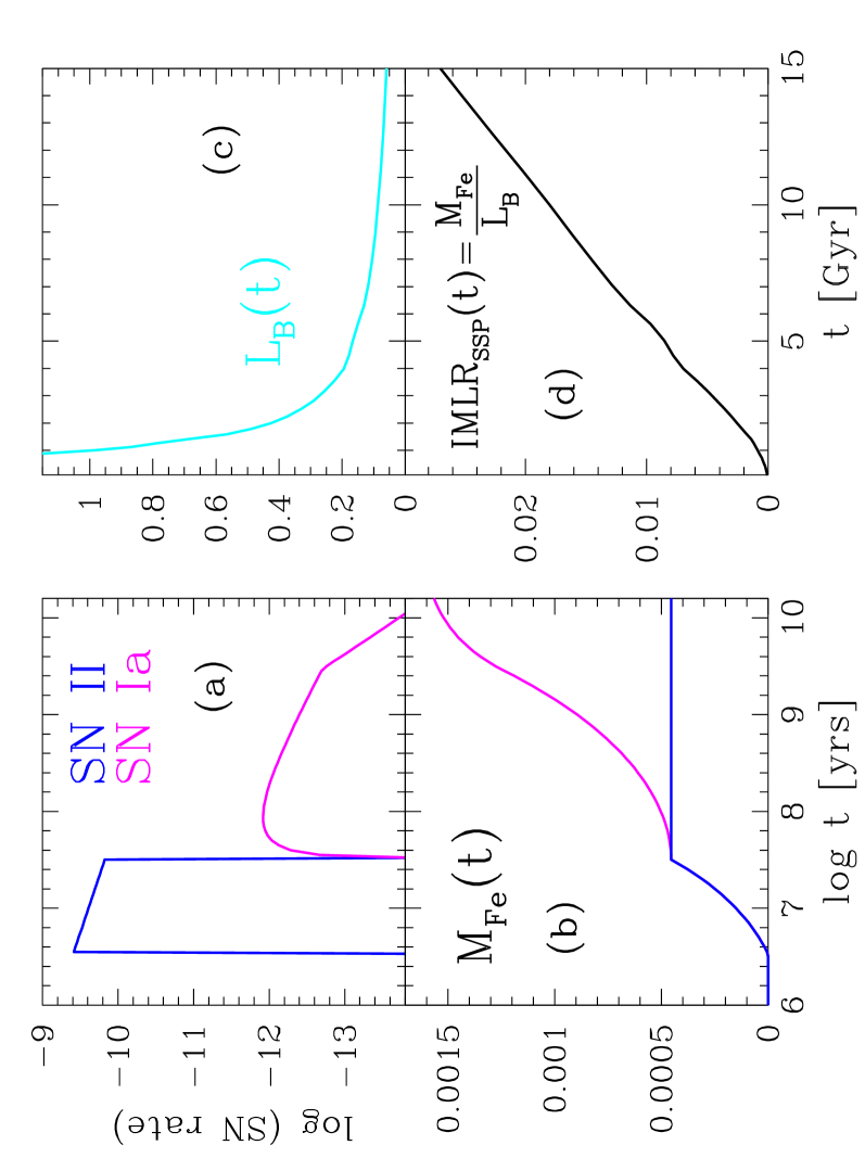
1 Introduction
The chemical enrichment of the intra–cluster medium (ICM) has been extensively discussed in literature by means of chemical evolution models of elliptical galaxies with galactic winds, and a variety of scenarios has been advanced (see the review by Matteucci, these proceedings). Very recently, cosmological hydro–dynamical simulations of cluster formation have been developed, that can follow self–consistently the star formation and chemical enrichment history of cluster galaxies and of the ICM (Valdarnini 2003; Tornatore et al. 2004; Romeo et al. 2004). Star formation has important effects on the hydro–dynamical evolution of the cluster, via energy feedback from supernovæ and metal enrichment of the ICM: the first effect contrasts, the second one boosts the cool-out of the hot gas. The chemical evolution of the ICM is not only an interesting issue per se, but an important ingredient of the global physical evolution of clusters. As a consequence, the choice of input parameters and “recipes” related to star formation (notably, the stellar Initial Mass Function and the implementation of sub–grid feedback effects) is crucial for the results of the simulations.
In this paper we outline a simple procedure to estimate the chemical enrichment of the ICM, the partition of the metals between stars and ICM, and the cold fraction expected after an assumed Initial Mass Function (IMF). This provides a guideline to select the optimal input parameters of the simulation; and to distinguish, in the results of a complex and fully self–consistent simulation, what is merely a consequence of the adopted IMF, and what is an effect of the interplay between hydrodynamical evolution and star formation.
2 IMF, metal production and partition between stars and ICM
Let’s choose an IMF and consider a burst of star formation (a Single Stellar Population, SSP) with stellar masses distributed accordingly; we can compute the expected rates of SN II and SN Ia, the corresponding rate of production of metals (for example, iron: ), and the luminosity evolution of the SSP . We can then define the Iron Mass–to–Light ratio typical of that IMF as IMLR. Fig. 1 illustrates this procedure for the Salpeter (1955) IMF with mass limits [0.1–100] M⊙; the detailed calculations can be found in Portinari et al. (2004, hereafter PMCS).
Part of the iron produced will be “eaten up” by subsequent star formation episodes, to build up the stellar metallicities observed in cluster galaxies; only the remaining fraction is available to enrich the ICM. We need to estimate how the total iron produced gets partitioned between the stellar populations and the ICM (Renzini et al. 1993).
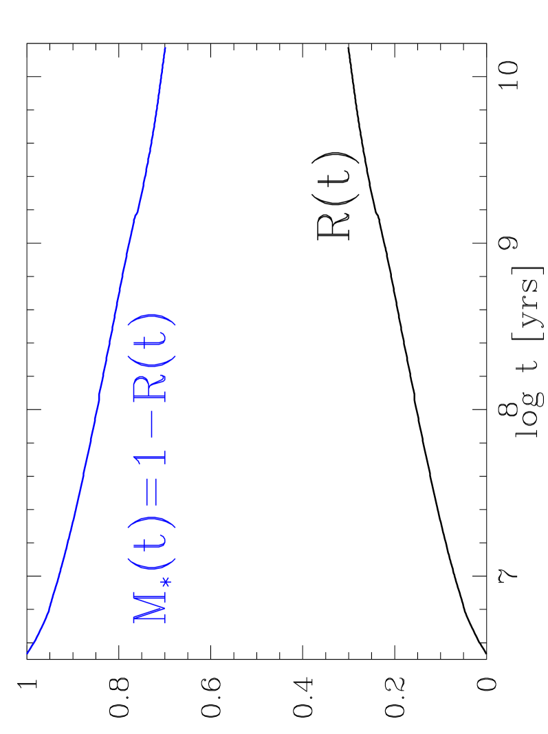
We can estimate the amount of iron locked in the stars as . As to the stellar metallicity , the star mass in clusters is dominated by massive ellipticals, with global metallicities between 0 (solar) and +0.2 dex, and [/Fe] ratios around +0.2 dex (PMCS and references therein). The mass in stars is not directly observable; it is usually inferred from the global luminosity of cluster galaxies, but the conversion factor, the stellar Mass–to–Light ratio (), depends on the IMF. Thus, the mass locked in stars is best computed self–consistently from the assumed IMF (Fig. 2); drives the actual amount of iron required to reproduce the observed metallicity .
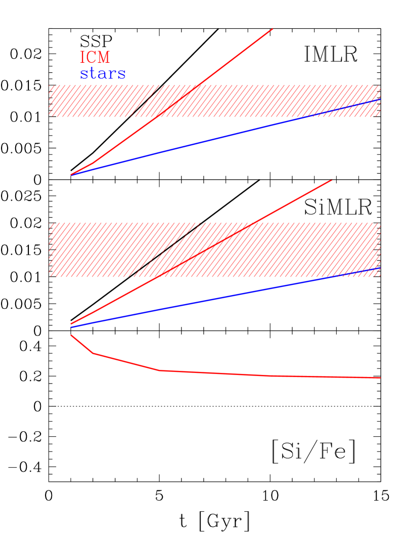
We are now able to split the characteristic IMLRSSP of the assumed IMF into the fraction IMLR locked in the stellar populations, and the remaining fraction IMLRICM that can be compared to ICM observations (Fig. 3a, red line vs. red shaded area). Notice that IMLRICM as computed here is an upper limit to the expected enrichment of the ICM, since all the iron not locked in the stars is assumed to be expelled from the galaxies. Whether this actually occurs, depends on the efficiency of extraction/ejection mechanisms (feedback, ram pressure, etc.).
The same exercise, described above for iron, can be repeated for any other element; in particular for the –elements that directly trace SN II enrichment and star formation. Among these, silicon is the best measured one in the ICM (Fig. 3b).
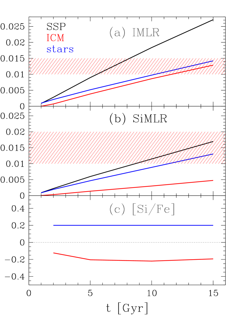
From Fig. 3, our simple argument shows that with the Salpeter IMF one expects:
-
1.
equipartition of iron between stars and ICM (Fig. 3a; Renzini et al. 1993);
-
2.
an IMLR in the ICM compatible with observations, provided the bulk of the stellar population in clusters is old (say, older than 10 Gyr; Fig. 3a);
-
3.
an uneven distribution (i.e. no equipartition) of –elements, that are mostly contained in the stars (Fig. 3b);
-
4.
a “chemical asymmetry” between stars and ICM (Fig. 3c; Matteucci & Vettolani 1988; Renzini et al. 1993; Pipino et al. 2002): the stars have supersolar [/Fe] abundance ratios — as we assumed a priori after observational results — while the ICM has undersolar [/Fe]; the latter result is at odds with observations (Finoguenov et al. 2000, 2001; Baumgartner et al. 2004);
-
5.
a SiMLR lower than observed (Fig. 3b).
In a hydro–dynamical simulation adopting the Salpeter IMF, these basic predictions can be used to check and interpret the results. For instance, if more iron is contained in the stars than in the ICM, it means that the simulated stellar iron abundances are in excess of the observed ones and a more efficient ejection of iron into the ICM needs to be implemented. If the IMLR in the simulated ICM is lower than observed, either not enough iron has been ejected into the ICM, or the stellar populations are too young (high luminosity); while a low SiMLR and an undersolar [Si/Fe] ratio in the ICM are expected with the Salpeter IMF and are not a fault of the simulations.
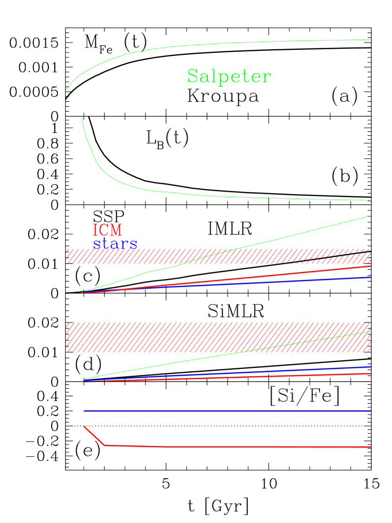
The results listed above refer to the Salpeter IMF, but the procedure can be applied to any other IMF; the expected metal production and partition between stars and ICM will be different. Fig. 4 shows the case for a typical Solar Neighbourhood IMF, the Kroupa (1998) IMF. With a steep Scalo slope at the high–mass end, the Kroupa IMF has a lower iron production than Salpeter (Fig. 4a). Being also “bottom–light” with respect to Salpeter (namely, with less mass locked in low–mass stars) it has a higher luminosity as well (Fig. 4b). All in all, its characteristic IMLRSSP is a factor of 2 lower than that of Salpeter, and it cannot possibly match the observed iron enrichment in the ICM (Fig. 4c; see PMCS for details). Even worse is the outcome for the –elements (Fig. 4d). Henceforth, one can predict beforehand that adopting a “standard” Solar Neighbourhood IMF in cluster simulations can never lead to a satisfactory ICM enrichment. Notice also that with the Kroupa IMF there is no equipartition of iron between stars and ICM (Fig. 4c); iron equipartition holds specifically for the Salpeter IMF.
Fig. 5 shows the expected production and partition of elements between stars and ICM, for the top–heavy Arimoto & Yoshii (1987) IMF (power–law exponent –1.0 vs. –1.35 for Salpeter; same mass limits [0.1–100] ). For this IMF, more metals are available to enrich the ICM than locked in the stars, and the IMLR and SiMLR in the ICM can match the observed levels for stellar populations of 5–10 Gyrs of age. The expected [/Fe] ratios in the ICM are supersolar, in agreement with observations. Therefore, a top–heavy IMF like this can potentially lead to satisfactory results; whether this is achieved in an actual simulation, depends on the simulated star formation history and ejection mechanisms of metals from the galaxies.
3 IMF, M∗/L ratio and cold fraction
In the previous section we showed that a self-consistent account of the mass and metals locked in the stars, related to the corresponding to the adopted IMF, is fundamental to predict the chemical enrichment of the ICM. The has also important consequences on the cold fraction, defined as the ratio between stellar mass and hot ICM gas mass (the cold gas component has a negligible mass contribution). The cold fraction is crucial to distinguish, for instance, the mechanisms responsible for the “entropy floor” in low temperature clusters. The larger the cold fraction, the larger the role played by galaxy formation that removes low entropy gas; with a small cold fraction, instead, strong supernova (pre)heating or other feedback sources are needed to set the entropy floor (Bryan 2000; Balogh et al. 2001; Valdarnini 2003; Tornatore et al. 2003). Consequently, a correct estimate of the cold fraction is a major constraint for scenarios of cluster evolution.
While can be inferred directly from the observed X-ray emission, the stellar mass can be estimated only indirectly from the observed luminosity, typically in the B–band, via an assumed . In literature, very discrepant values can be found for the cold fraction — or its reciprocal:
This discrepancy is mostly due to the assumed ; the determinations of the directly observed quantity (listed below as compiled by Moretti et al. 2003) are in much better agreement, within 30% around:
| 30 | David et al. (1990), Hydra A |
|---|---|
| 30 ( 13) | Arnaud et al. (1992) |
| 30 | White et al. (1993), Coma |
| 19 | Cirimele et al. (1997) |
| 31–44 | Roussel et al. (2000) |
| 21 | Finoguenov et al. (2003) |
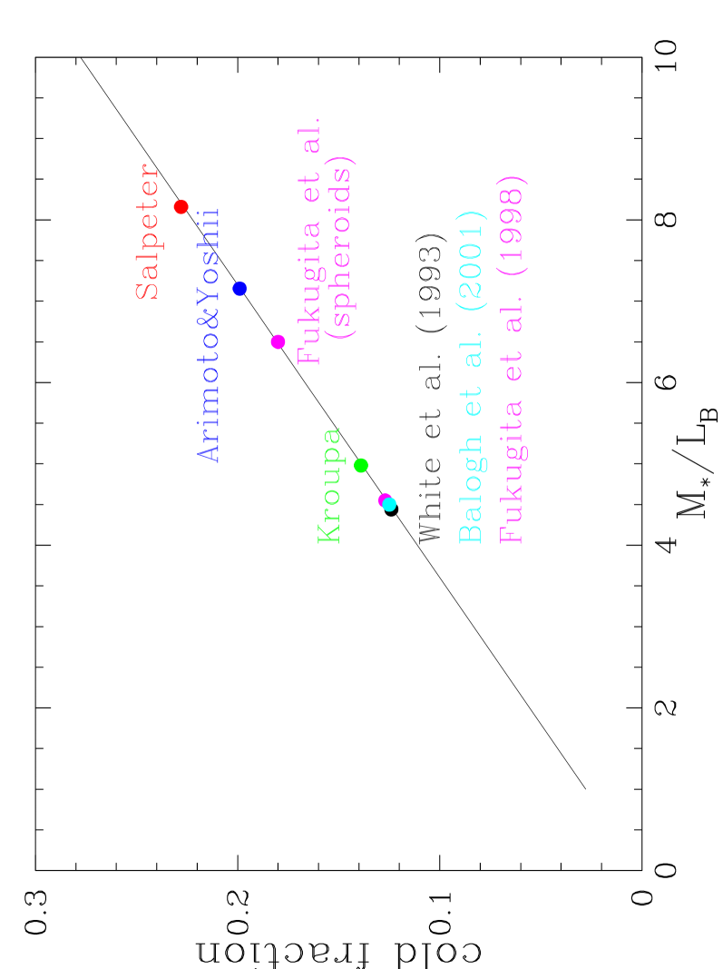
With this typical value of , the cold fraction depends on the assumed as shown in Fig. 6. Displayed are the values of assumed by White et al. (1993) and Balogh et al. (2001), by Fukugita et al. (1998; averaged over the typical morphological mixture of cluster galaxies out to the Abell radius, or for spheroids only); and the values corresponding to the Salpeter, Kroupa and Arimoto & Yoshii IMF, assuming an age of 10 Gyr for the stellar populations. The estimated cold fraction ranges between 10 and 20%; while such factor of 2 is of little relevance for the “baryon budget” addressed by White et al. and Fukugita et al., since the baryonic mass in clusters is anyways largely dominated by the hot ICM, it has a drastic impact on chemical enrichment, cold fraction and cluster modelling. Fig. 6 shows that, if one assumes a Salpeter (or Arimoto & Yoshii) IMF, the observed corresponds to a cold fraction around 20% for suitable ages of the stars in cluster galaxies (10 Gyr, suited to reproduce the IMLR: Fig. 3a). The widely quoted cold fraction of 10% can be reached only by simulations that assume an IMF corresponding to values as low as assumed by e.g. White et al. (1993).
The correct constraint for a simulation is the cold fraction corresponding to the assumed IMF, based on the observed . Equivalently, for the simulated cluster one can compute self–consistently the luminosity relevant to the assumed IMF and compare directly to the observed .
Alternatively, if simulations aim at reaching a cold fraction of 10%, one should select beforehand an IMF (quite “bottom light”) able to reach as low values of as assumed by White et al., for the old ages typical of elliptical galaxies.
4 Conclusions
We remark the following crucial points for modelling the cosmological evolution and chemical enrichment of clusters of galaxies self–consistently.
-
•
The amount of mass and metals locked in the stellar component is not necessarily negligible, depending on the assumed IMF and corresponding .
-
•
The observed metal content in stars can be used as a constraint for the efficiency of feed–back and of metal dispersion in the simulations: the wind efficiency cannot be indefinitively enhanced, because the amount of metals in the stars should also be accounted for, and a sizable fraction of the metals produced may thus not be available to enrich the ICM. (Though the problem of present–day simulations is rather the opposite, namely to lock too much metals in the stars; Tornatore et al. 2004; Romeo et al. 2004).
-
•
Once an IMF is chosen for the simulations (preferably a bottom–light IMF with high-mass slope shallower than Scalo, see PMCS), we suggest to compute the corresponding partition of metals between stars and ICM with the simple procedure outlined in this paper. Such expected partition can then be used to test the numerical results.
-
•
The crucial constraint of the cold fraction should be consistent with the relevant to the assumed IMF. As the observational quantity is luminosity, we suggest to compute the luminosity of the simulated cluster consistently with the adopted IMF, and compare it directly to the observed . Red or IR luminosities are preferred, since they probe the stellar mass with a lower sensitivity to the age of the stellar populations and to recent star formation activity; estimates are becoming available (Lin et al. 2003).
References
- (1) Arimoto N., Yoshii Y., 1987, A&A 173, 23
- (2) Arnaud M., Rothenflug R., Boulade O., Vigroux L. & Vangioni-Flam E., 1992, A&A 254, 49
- (3) Balogh M.L., Pearce F.R., Bower R.G. & Kay S.T., 2001, MNRAS 326, 1228
- (4) Baumgartner W.H., Loewenstein M., Horner D.J. & Mushotzky R.F., 2004, ApJ submitted (astro-ph/0309166)
- (5) Bryan G., 2000, ApJ 544, L1
- (6) Cirimele G., Nesci R. & Trevese D., 1997, ApJ 475, 11
- (7) David L.P., Arnaud K.A., Forman W. & Jones C., 1990, ApJ 356, 32
- (8) Finoguenov A., David L.P. & Ponman T.J., 2000, ApJ 544, 188
- (9) Finoguenov A., Arnaud M. & David L.P., 2001, ApJ 555, 191
- (10) Finoguenov A., Burkert A. & Böhringer H., 2003, ApJ 594, 136
- (11) Fukugita M., Hogan C.J. & Peebles P.J.E., 1998, ApJ 503, 518
- (12) Kroupa P., 1998, ASP Conf. Series 134, 483
- (13) Lin Y.-T., Mohr J.J. & Stanford S.A., 2003, ApJ 591, 749
- (14) Matteucci F. & Vettolani G., 1988, A&A 202, 21
- (15) Moretti A., Portinari L. & Chiosi C., 2003, A&A 408, 431
- (16) Pipino A., Matteucci F., Borgani S. & Biviano A., 2002, NewA 7, 227
- (17) Portinari L., Moretti A., Chiosi C. & Sommer–Larsen J., 2004, ApJ in press (astro-ph/0312360) (PMCS)
- (18) Salpeter E.E., 1955, ApJ 121, 161
- (19) Renzini A., Ciotti L., D’Ercole A. & Pellegrini S., 1993, ApJ 419, 52
- (20) Romeo A.D., Sommer-Larsen J., Portinari L. & Antonuccio V., 2004, in preparation
- (21) Roussel H., Sadat R. & Blanchard A., 2000, A&A 361, 429
- (22) Tornatore L., Borgani S., Springel V., Matteucci F., Menci N. & Murante G., 2003, MNRAS 342, 1025
- (23) Tornatore L., Borgani S., Matteucci F., Recchi S. & Tozzi P., 2004, MNRAS in press (astro-ph/0401576)
- (24) Valdarnini R., 2003, MNRAS 339, 1117
- (25) White S.D.M., Navarro J.F., Evrard A.E. & Frenk C.S., 1993, Nature 366, 429