The highest-energy cosmic rays

Talk presented at TAUP 2003, Seattle, USA

Abstract

This is a review of the experimental data concerning the spectrum, arrival distribution and composition of cosmic rays with energies $\geq$ 10¹⁹ eV. Before the experimental review I briefly discuss the conditions for the production followed by a review of the propagation of cosmic rays. Then follows a discussion of the properties of the showers produced by the primary cosmic ray particles and a description of the techniques used to detect the showers and extract the energy, direction and nature of the primary. The main conclusion of the experimental review is that there is still insufficient data to answer all the questions concerning the particles which strike the earth with such enormous energies. There has been significent progress which I will discuss and there are good prospects that in the next five years we will come much closer to the answers. Much more can be learned from existing data but a more sophisticated and disciplined analysis will be required.

1 Introduction

Over the past ten years the interest in the nature and origin of the highest-energy cosmic rays, those with energy $\geq 10^{19}$ eV, has grown enormously. Of particular interest are cosmic rays with energy $\geq 10^{20}$ eV. At these energies the cosmic ray particles, be they protons, nuclei, or photons, interact strongly with the cosmic microwave background and should be severely attenuated, except for those whose sources are in our cosmological neighborhood ($\leq$ 100 Mpc). Also protons of these energies may not be significantly deflected so that some of the cosmic rays may point back to their source. A recent authoritative review by Nagano and Watson [1] presents the experimental and theoretical background. For all but the most recent references I refer the reader this article.

I dedicate this article to the memory of John Linsley (b. March 12, 1925; d. September 15, 2002). He discovered the first cosmic ray with an energy of $10^{20}$ eV [2] 42 years ago. John Linsley has contributed so much to our understanding of cosmic ray showers. Many of his contributions are tucked away in old proceedings of cosmic ray conferences. His original development of the concept of elongation rate is to be found in the Proceedings of the 15th ICRC held in Plovdev, Bulgaria [3]. (The elongation rate is referred to in section 3 and section 5.3 of this paper.) Up until his death he was active in all aspects of cosmic ray physics. He was the founder of the idea for a satellite-borne fluorescence telescope, which is being realized in the EUSO detector to be placed on the Space Station.

He considered me an upstart when I began with colleagues to argue for a really large surface detector’ one which ultimately became the Auger Observatory. However with the passage of time I believe I gained his respect. I only wish that he could witness the progress that is going to be made. I cannot avoid the fantasy that he is now in a position to know all the answers!

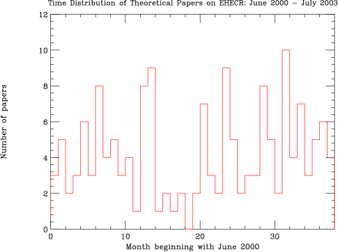
Figure 1: Number of theoretical and speculative papers on the subject of the highest-energy cosmic rays.

Figure 2: Some titles of paper concerning the highest-energy cosmic rays.

Much more data will be required to understand the mystery behind the existence of cosmic rays with such extraordinary energies. An article by Michael Hillas [4], published nearly twenty years ago, presented the basic requirements for the acceleration of particles to energies $\geq 10^{19}$ eV by astrophysical objects. The requirements are not easily met, which has stimulated the production of a large number of creative papers.

In Figure 1 I plot the number of theoretical papers, mostly speculative, written on the subject of the highest-energy cosmic rays as a function of time, as found on the Los Alamos server as astro-ph papers. Over the last three years the average has been one paper per week. In Figure 2 I list a random sample of the titles. The authors of these papers deserve a strong response from the experimental community.

Figure 3: Panorama of the interactions of possible cosmic primaries with the CMB. Curves marked by “p+$\gamma_{CMB}$ $\rightarrow$ e⁺e^-+p” and “Fe+$\gamma_{CMB}$ $\rightarrow$ e⁺e^-+p” are energy loss lengths (the distance for which the proton or Fe nucleus loses 1/e of its energy due to pair production). The curve marked by “p+$\gamma_{CMB}$ $\rightarrow$ $\pi^{+}$n or $\pi^{\circ}$p” is the mean free path for photo-pion production of a proton on the CMB. The curve marked “Fe+$\gamma_{CMB}$ $\rightarrow$ nucleus + n or 2n” is the mean free path for a photo-nuclear reaction where one or two nucleons are chipped off the nucleus. The curve marked “$\gamma$ +$\gamma_{CMB}$ $\rightarrow$ e⁺e^-” is the mean free path for the interaction of a high-energy photon with the CMB. Added for reference is the mean decay length for a neutron indicated by “n $\rightarrow$ pe$\nu$”.

2 Propagation of the highest-energy cosmic rays

The interaction of the particles with the cosmic microwave background (CMB) and magnetic fields plays an important role in their propagation. All possible species of cosmic rays with the exception of neutrinos interact with the CMB. A panorama of the various interactions is given in Figure 3.

Figure 4: Mean energy of protons as a function of propagation distance through the CMB. Curves are for energy at the source of 10²² eV, 10²¹ eV, and 10²⁰ eV.

Figure 5: Fluctuation of the energy of a proton propagating through the CMB.

The most discussed is the Greisen-Zatsepin-Kuzmin (GZK) effect [5], where a cosmic ray proton interacts with a CMB photon. The collision of a $10^{20}$ eV proton with a $10^{-3}$ eV photon produces about 200 MeV in the center of mass, which is the peak for photo-pion production. These collisions produce a neutron and charged pion or a proton and neutral pion with significant loss of energy for the nucleon. The neutron mean decay length is 1 Mpc at 10²⁰ eV so on the Mpc scale it quickly becomes a proton again. The mean energy of a nucleon as a function of propagation distance through the CMB is shown in Figure 4. The interaction of a nucleon with the CMB is a stochastic one where a significant amount of energy can be lost in a single collision. As a consequence the fluctuation of the energy of a nucleon about the mean as a function of distance is large. The fluctuation about the mean is shown in Figure 5.

Figure 6: Probability that an observed event at a given energy has its source at a distance greater than the indicated distance. A source spectrum proportional to E^-2.5 is assumed. Figure provided Paul Sommers, University of Utah.

While these two figures present the physics of propagation of protons in the CMB, the observer has to answer the inverse question. If a cosmic ray is observed with a particular energy, what is the probability that it came from a distance greater than a specified amount? To compute this probability requires an assumption about the spectrum at the source. With an assumed source spectrum of E^-2.5 the probability is plotted in Figure 6. The GZK interaction begins to have a significant effect at an energy of 8 x 10¹⁹ eV where there is only a 10$\%$ probability that the cosmic ray traveled a distance greater than 100 Mpc. Cosmic rays at lower energies can traverse much greater distances with little energy loss, but it is also possible that such a cosmic ray was produced at a higher energy and encountered a CMB photon at a great distance.

Since the energy loss in the collisions with the CMB has such large fluctuations, a set of data with a small number of events above 10²⁰ eV will have fluctuations far in excess of simple Poisson statistics. The importance of these fluctuations has been discussed in a recent paper [6], which demonstrates that none of the experiments done up to the present have the statistical power to address the existence of a GZK cutoff. But I must stress that a single event observed with energy 3 x 10²⁰ eV has about a 0.1$\%$ chance of having traveled more than 50 Mpc.

The expectation of the number and spectrum of post-GZK events is not a simple calculation, since the distribution of possible sources within 100 Mpc may not be treatable as a continuum. The distribution of nearby sources is certainly not identical as one looks in different directions of the sky. For this reason, a comprehensive study of these highest-energy cosmic rays requires the observation of the entire sky. One cannot assume that the spectrum at its upper end is independent of the direction of observation.

A major portion of the cosmic rays is charged particles. There is evidence, not yet conclusive, that protons are the predominant species above 10¹⁹ eV. The Larmor radius of a charged particle with atomic number Z is:

$\rho$(Mpc)=1.08x10²$\cdot$(E/10²⁰eV)$\cdot$(1/B_ng)$\cdot$(1/Z).

A proton of 10¹⁹ eV in the galactic magnetic field of about 1 $\mu$-gauss has a Larmor radius of 10 kpc, large compared to the thickness of the galaxy. Thus, if a proton of such an energy is born in the galactic disk, it will immediately escape. Iron nuclei of that energy will linger in the galaxy but will show an anisotropy if they are born in the galactic disk. As there is no correlation of the arrival directions of $\geq$ 10¹⁹ eV cosmic rays with the galactic disk it appears that their sources are either extragalactic or originate in an extended halo of the galaxy.

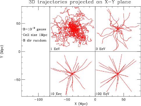
Figure 7: Projected view of 20 trajectories of proton primaries emanating from a point source for several energies. Trajectories are plotted until they reach a physical distance from the source of 40Mpc. See text for details.

Not a great deal is known about magnetic fields outside of galaxies. In clusters of galaxies such as the Virgo cluster the fields can be of the order of a $\mu$-gauss [7]. With exaggerated symplicity these fields are often described by cells of size $\lambda$ = 1Mpc with mean value B oriented randomly in each cell. This is the model taken for the measurement of the magnetic fields by Faraday rotation [8]. In the voids or near voids of extragalactic space an estimate of the magnitude of the randomly oriented magnetic field is $\leq$ 1 nanogauss.

I have made some simple calculations to give a feeling of the very important effects that even such a small field can have on the propagation of charged cosmic rays [9]. In Figure 7 I have plotted in plane projection twenty 3-dimensional trajectories for cosmic ray protons emitted from a point source. The trajectories are followed until they reach a spatial distance of 40 Mpc from the source. The actual traversed distance which is relevant for the various energy loss processes can be much longer. No energy loss was applied in these calculations. One can see that for the assumed magnetic conditions the propagation of the cosmic rays passes from diffusive propagation to rectilinear propagation in passing from 1 EeV to 100 EeV. (I hope the reader will excuse the shift in energy units here, 1 EeV = 10¹⁸ eV) These graphs can be easily scaled for other magnetic conditions. For example, if the magnetic field were 100 nanogauss, propagation at 100 EeV would be completely diffusive, as shown in the upper left panel of Figure 7. Propagation at 1000 EeV however would be quite distinct from the lower left panel as energy loss by the GZK effect would be significant. Less than 1$\%$ of the particles would escape interaction with the CMB and propagate rectilinearly. The remainder would quickly pass to diffusive propagation, drop below 100 EeV, and travel much more slowly from the source. For iron primaries, the panel on the upper right of Figure 7 would correspond to 80 EeV. This regime is not fully diffusive and the primaries would have some memory of their source which would be revealed by a broad anisotropy. These examples reveal the complexity introduced in propagation of cosmic rays due to magnetic fields. In some cases the galactic magnetic field will also be important.

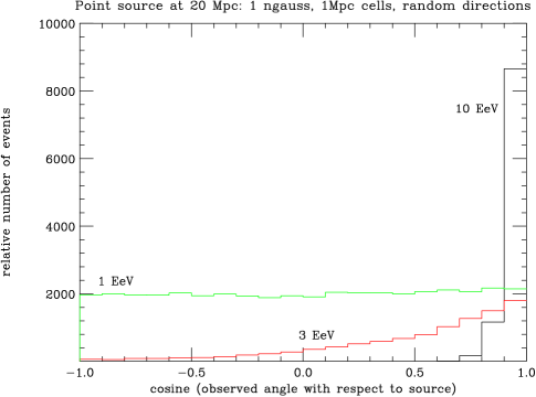
Figure 8: Distribution at 20 Mpc distance of the observed cosmic ray angle with respect to the source direction for proton primaries at the indicated energies.

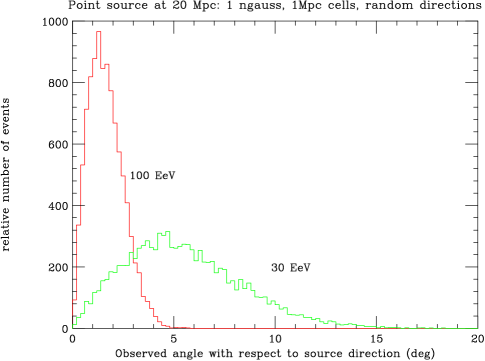
Figure 9: Distribution at 20 Mpc distance of the observed cosmic ray angle with respect to the source direction for proton primaries for the cases of small deflection.

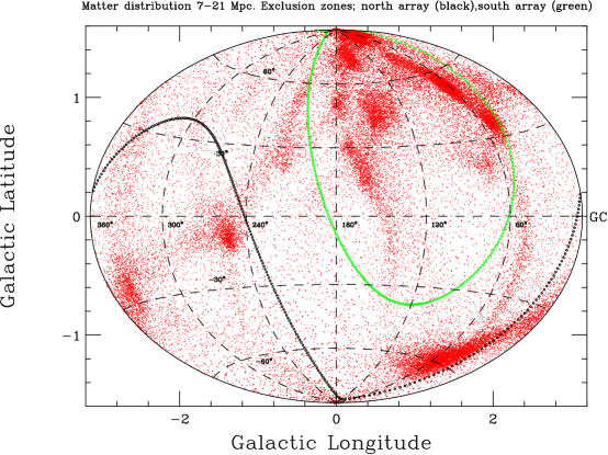
Figure 10: Distribution in galactic coordinates of gravitating matter at distance between 7 and 21 Mpc. The density of dots in the figure is proportional to the column density of the matter in the interval. The exclusion zones are plotted for a zenith angle $\leq$ 60$\deg$. On the left is the exclusion zone for a northern observatory, on the right for a southern observatory. An observatory in the southern hemisphere will not see directly the Virgo cluster. (The data were provided by Andrey Kravtsov, Center for Cosmological Physics, University of Chicago).

In Figure 8 I have plotted the distribution of observed directions of the cosmic rays with respect to the source direction. For 1 EeV proton primaries the directions are completely isotropic; no memory of the source direction remains. In Figure 9 I plot the dispersion of angles for 100 EeV and 30 EeV proton primaries. Here the angular spread is 1.5^∘ and 5^∘ respectively.

If the sources of cosmic rays with energy $\geq$10 EeV are extragalactic and are associated with the distribution of nearby matter, then one would expect that the flux and energy spectrum of the cosmic rays will depend on the hemisphere in which the observations are made. Most of the nearby matter is found in the Virgo cluster at a distance of $\sim$ 18 Mpc. In Figure 10 I plot the column density of gravitating matter between 7 and 21 Mpc. Also plotted in the figure are the exclusion zones for observatories at 35^∘ north and south latitude. The bulk of the Virgo cluster is not seen by an observatory in the southern hemisphere.

3 Properties of showers

When a cosmic ray strikes the earth’s atmosphere a shower of particles is produced. In this section I describe the properties of these showers with emphasis on the features that are important for the detection, and measurement of the energy, direction, and nature (proton, nucleus, or photon) of the primary cosmic ray. These properties are derived from both simulations [10] and data from the Engineering Array of the Pierre Auger Observatory [11]. This discussion concerns showers with zenith angles of less than 60^∘. Steeper showers, often referred to as horizontal showers, begin to be dominated by muons as the electromagnetic component quickly dies out. The method to analyse horizontal showers is discussed in an Auger Observatory paper [12], and is beyond the scope of this paper.

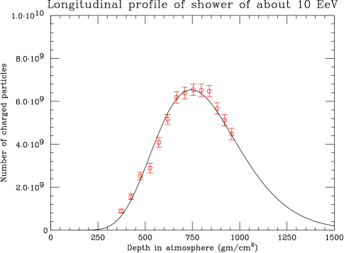
Figure 11: Longitudinal development of a 9 EeV shower in the atmosphere. The solid line is an empirical fit to the shower development. The red points are the measurements of the shower development by detection of its nitrogen fluorescence.

In Figure 11 we show the longitudinal development of a shower of energy about 10 EeV. The solid curve is an empirical shape proposed by Gaisser and Hillas [13]. The points are a measurement by one of the fluorescence telescopes of the Pierre Auger Observatory. As will be discussed below the longitudinal development in the atmosphere can be directly measured by observation of nitrogen fluorescence. A 10¹⁹ eV shower produces about 7 x 10⁹ charged particles at its maximum development. Most of the shower particles are very close to an axis defined as the direction of the primary particle. Roughly 80$\%$ of the particles are within one Molière radius of the shower axis. This radius, measured in radiation lengths, is the ratio of the multiple scattering constant, 21.2 MeV to the critical energy in air, 80 Mev. Typically this distance is about 100 meters.

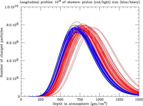
Figure 12: Simulated shower profiles for proton (light profiles) and iron (heavy profiles).

The energy of the shower can be obtained by integration of the ionization loss in the atmosphere, given, approximately, by 2.2$\int$$N_{e}$(x)dx MeV, where 2.2 MeV/gm/cm² is dE/dx for electrons at the critical energy, $N_{e}$(x) is the number of shower particles at the atmospheric depth x gm/cm². Implicit in this formula is the presumed knowledge of the shape of the longitudinal development outside the range of measurement. Also some energy is not observed in the form of neutrinos and penetrating muons. Accounting for this energy adds about 7$\%$ to the ionization energy for a 10¹⁹ eV shower.

The position of the shower maximum, X_max, fluctuates principally because the depth of the first interaction fluctuates. For a proton induced shower the fluctuation is the largest. For a heavy nucleus like iron, X_max is less and the fluctuations are less. This is best understood by considering an iron shower being produced by 56 nucleons of 1/56th the energy. As discussed in the following paragraph, X_max grows with energy. Thus, for an iron shower, X_max is less and the fluctuations are less because one has the averages over 56 showers. Simulations show that conclusions derived from this superposition model are remarkably accurate. The model permits one to make simple semi-quantitative arguments for the comparison of shower properties. Reading the cosmic ray literature might suggest that the only hadronic components of cosmic rays are protons and iron nuclei. Of course this is not the case as many nuclear species between proton and iron are found in the cosmic rays. Protons and iron represent the extremes. A number of simulated proton and iron shower profiles is shown in Figure 12. The X_max for the iron showers is less deep and the fluctuations for the iron showers are smaller. The mean X_max and its standard deviation for protons is 780 and 53 gm/cm², for iron nuclei 700 and 22 gm/cm².

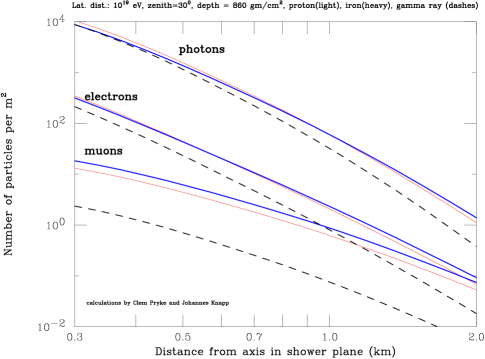
Figure 13: Simulations of the lateral distribution of shower particles. The curves are averages over many showers. These are the densities in the plane perpendicular to the axis of 10¹⁹ eV proton, iron, or gamma ray initiated showers.

An important quantity obtained from the longitudinal shower development is the elongation rate dX_max/dlogE, the increase in X_max per decade. This concept was first introduced by John Linsley [3]. For pure electromagnetic showers, X_max = X₀ln(E/E_c) so that dX_max/dlogE = 2.3X₀ = 84 gm/cm²/decade. Here E_c = 80 MeV is the critical energy in air and X₀ = 36 gm/cm² is the radiation length in air. For hadron primaries with a multiplicity that grows with energy, the elongation rate is much less. To illustrate the point consider a model in which the first interaction produces N(E) neutral pions. This is like 2N electromagnetic showers of energy E/2N. Then X_max = X₀ln(E/2NE_c) and dX_max/dlogE = 2.3X₀(1-dlnN/dlogE). The rate of increase in the depth of X_max is decreased. Elongation rates around 10¹⁹ eV are about 60 gm/cm²/decade. The superposition model would predict difference in X_max between iron and proton to be log(56) x 60 = 100 gm/cm² compared to 80 in the simulations. Both the mean value of X_max and its fluctuation potentially carry information about the primary composition.

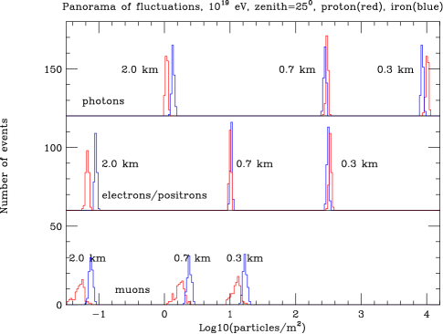
Figure 14: Density fluctuations of shower particles for selected distances from the shower axis. The light histograms are for protons and the heavy histograms iron.

An array of particle detectors spread out on the ground is sensitive to the lateral distribution of the shower particles. The lateral distributions for showers initiated by protons and iron nuclei are shown in Figure 13. These curves are the result of simulations. While the quantitative results depend somewhat on models the qualitative result is unchanged. Plotted are the average distributions of 100 showers. The principal components are photons, electrons and muons. There are hadrons near the shower core but their contribution is negligible at more than a few 100 meters. One should note that the density of photons and electrons is almost identical for proton and iron initiated showers in the range from 500 to 1000 meters from the core. The iron initiated showers develop higher in the atmosphere so the particles are spread more broadly than in a proton initiated shower. However as the iron initiated shower particles have a greater distance to travel than the proton initiated ones there is more attenuation. The two effects compensate one another. The gamma ray initiated showers are distinctly different. These showers have a much steeper lateral distribution because they develop much deeper in the atmosphere and they have many fewer muons. These characteristics make the identification of a gamma ray initiated shower easier. The gamma ray showers have muon densities about a factor five lower than protons of the same energy. The exact factor depends on the strength of the gamma ray production of hadrons. This strength has to be extrapolated from lower-energy data. Nevertheless, one expects many fewer muons in gamma ray initiated showers.

The muon densities are different for protons and iron, but not by a large amount. Iron initiated showers produce about 1.45 times more muons than proton initiated showers [14]. This ratio can be understood qualitatively through the superposition model. Empirically it is known that the ratio of muons to electromagnetic particles increases more slowly than the energy. Typically this ratio goes as E^.92. Taking iron showers to be 56 proton showers each of 1/56th the energy, one finds the ratio to be $\sim$ 56^1-.92 = 1.38, a reasonable agreement. Simulations using different interaction models predict electromagnetic densities that vary at most by perhaps 20$\%$. However different models can predict muon densities which can vary by as much as a factor 2. The qualitative conclusion however remains that the muon to electromagnetic ratio increases with atomic number.

At large distances from the core the intrinsic density variations due to fluctuation in the shower maximum are rather small. Examples of these fluctuations are plotted in Figure 14. The fluctuation of the electromagnetic component is about 4$\%$ RMS. The fluctuation of the muon component is larger being about 20$\%$ RMS for proton induced showers and 10$\%$ RMS for iron induced showers. These intrinsic fluctuations are generally not the limiting factor which determines the precision of the air shower detectors.

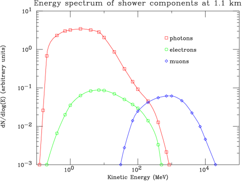
Figure 15: Energy spectrum of the shower components at 1.1 km. The spectrum of the electromagnetic components does not vary much beyond 1 km. At 2 km the peak of the muon spectrum is shifted from 1 GeV to 600 MeV.

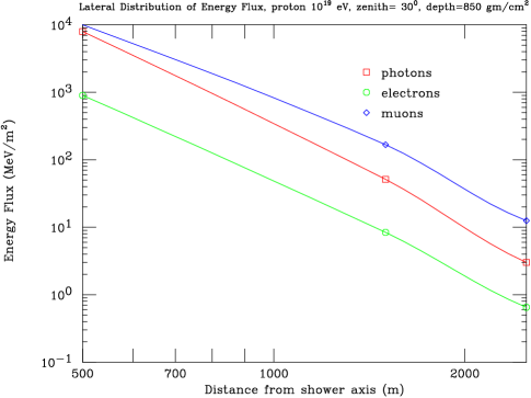
Figure 16: The lateral distribution of the integrated energy flux for each shower component.

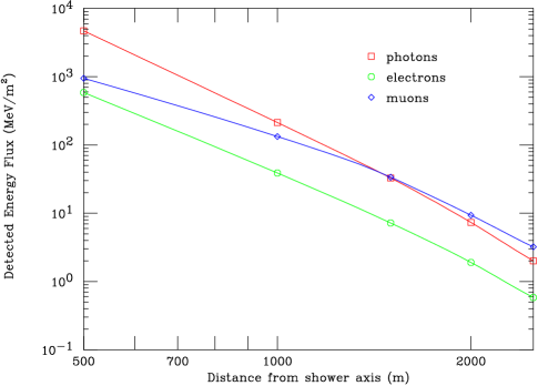
Figure 17: The lateral distribution of the detected energy flux for each shower component.

A scintillator detector responds to the number of ionizing particles that pass through it. If there is little material above, the scintillator records only the electrons and muons. The density of particles at 600 meters is related to the primary energy and, following Figures 13 and 14, this density is relatively insensitive to the nuclear composition.

Tanks of water have also been used as particle detectors using the Cherenkov radiation produced by the charged particles [15]. They are also very efficient in detecting the photon component of the shower. A deep water detector responds more directly to the energy flux of the shower particles. The energy distribution of the shower particles is shown in Figure 15. The integrated energy flux as a function of distance from the shower axis is shown in Figure 16. The energy flux far from the core is carried principally by the muons. The energy flux actually detected in 1.2 meters of water is shown in Figure 17. Water tanks of 10 m² in area and 1.2 m deep will be used as surface detectors in the Auger Observatory. This shape has the property that the average energy deposit of each shower component is nearly independent of the zenith angle out to 60^∘.

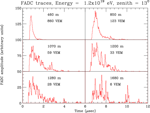
Figure 18: FADC traces for a $\sim$10¹⁹ eV shower. The zenith angle of the shower is 13^∘ indicating a young shower. Each panel shows the trace measured in an Auger water tank at the indicated distance. The strength of the signal is also indicated. The start time of each trace is arbitrary. The trace at 1680 m shows evidence of individual muons.

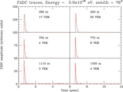
Figure 19: FADC traces for a $\sim$5x10¹⁸ shower. The zenith angle of the shower is 76^∘ indicating an old shower. Each panel shows the trace measured in an Auger water tank at the indicated distance. The strength of the signal is also indicated. The start time of each trace is arbitrary.

There is an additional property of showers that has yet to be fully exploited [16]. This is the fact that the shower particles arrive spread out in time as they are detected away from the shower axis. The spread in time of the particles beyond 1.0 km is measured in $\mu$-sec and is approximately proportional to the the distance to the shower axis. The energy deposited by the shower particles in the Auger water detectors is recorded in individual time slots of 25 ns width. Fast analog to digital convertors (FADCs) are used for this purpose. This energy deposit is measured in units of VEM, (vertical equivalent muons, the signal produced by a single muon traversing the center of the tank). The distribution of arrival times for a shower with zenith angle of 13^∘ is shown in Figure 18. This shower of about 10¹⁹ eV is called “young” as its maximum occurs at about 750 gm/cm² close to the ground level of 850 gm/cm². By contrast large zenith angle showers present a strikingly different pattern as shown in Figure 19. Here the particles arrive within a fraction of a $\mu$-sec for a shower with zenith angle 76^∘. This shower is called “old” as it is observed after having passed through 3500 gm/cm² before reaching the ground. These old showers consist entirely of muons (with $\sim$ 20$\%$ electromagnetic fuzz clinging to them) and have a very sharp shower front. The electromagnetic part of the shower has died out. One can note as well that the young shower has a much steeper lateral distribution, a signal ratio of 140 for a distance ratio of 3.6. For the old shower the signal ratio is only 4 for a distance ratio of 3.5.

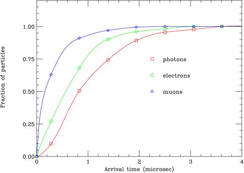
Figure 20: Integral arrival time for the components of a young shower of 10¹⁹ eV. The distance to the shower axis is 1 km.

The shape of the trace for young showers contains information about the relative amount of muons and electromagnetic particles in the shower. Figure 20 shows a simulation of the integrated arrival times for muons, electrons and photons for a typical young shower initiated by a proton of 10¹⁹ eV. Geometrical arguments lead to the conclusion that the more distant the shower maximum is from the ground, the tighter the spread of particles. Iron primaries have a more distant shower maximum and more muons, which will result in a sharper pulse. Analysis of the shapes of FADC traces can help reveal statistically the nature of the primary particle.

4 The two large experiments

There are two cosmic ray experiments that now dominate the experimental scene. The most mature of the two in its analysis and the best documented is AGASA (Akeno Giant Air Shower Array) [17]. AGASA operated for 12 years and ceased operation January 4, 2004. The High Resolution Fly’s Eye (HiRes) has been operating for a few years and will continue through 2005. It is a stereo fluorescence detector and the analysis is at present less mature than AGASA.

4.1 AGASA

The design of the AGASA was made in the late 1980’s before the availability inexpensive FADCs. The particle densities were measured logarithmically. The calibration was based on measurements of single muons in the cosmic rays. A number of technical criticisms accumulated over the years concerning the response of the electronics and the sensitivity of scintillators to delayed slow neutrons associated with the shower. The reference [17] addresses in a satisfactory way these criticisms, and the reader is encouraged to consult this paper.

AGASA was a surface array consisting of 111 scintillator detectors spread over an area of 100 km². The scintillators are 2.2 m² in area and 5 cm thick. In addition there are 27 muon detectors in the southern part of the array. These are shielded particle detectors ranging in area from 2.8 to 10 m². The mean atmospheric depth is 920 gm/cm². The most recent report was based on an exposure of 5.3 x 10¹⁶ meter²-sec-sr for showers with zenith angles less than 45^∘ [18].

The shower energy is proportional to the density of particles recorded at 600 meters. The scintillator measures almost exclusively the electron component of the shower. The sensitivity to the photon component is less than 10$\%$. The contribution of muons to the signal at 600 meters is about 10-14$\%$, referring to Figure 13. The signal at 600 meters is insensitive to the primary composition and on average independent of the position of shower maximum. It was Hillas [19] who first pointed out that the density at 600 meters is a good energy parameter. The distribution of shower particles is at any depth cylindrically symmetric in a plane perpendicular to the shower axis. However the plane of the ground is only concident with a shower plane for vertical showers. The signals are placed in an effective shower plane by plotting their perpendicular distances to the shower axis. For inclined showers an azimuthal asymmetry is generated about the shower axis. For a shower of inclination of 30^∘ the atmospheric depth at 600 meters from the shower axis is modulated by $\pm$40 gm/cm² and at 45^∘ by $\pm$70 gm/cm². These azimuthal variations are ignored. As the showers are near maximum development and as in most events a number of azimuths are sampled, the modulation usually averages out.

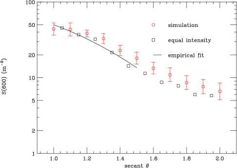
Figure 21: Dependence of the particle density at 600 meters for the AGASA array on zenith angle for showers of 10¹⁹ eV. Shown are the experimentally measured points using the equal intensity method. The solid line is the empirical fit used to obtain S₀(600), the equivalent value for a vertical shower. Also shown are the points produced by simulation. The absolute values are normalized by the simulation.

What is important however is the general attenuation of the entire shower, since the atmospheric depth increases with inclination. This attenuation, at energies where there are many showers, can be directly measured. For a given energy the true flux of cosmic rays should be independent of the zenith angle. By selecting showers in bins of zenith angle and demanding equal rates, one can relate the density of particles at 600 m with that for vertical showers, and thus determine for a given energy the density as a function of zenith angle. This “equal intensity” method can be checked by simulations. The measured relative response and the results of simulations for the AGASA array are shown in Figure 21. Also plotted is the empirical relation used to convert the observed density to what its value would be for a vertical shower. That density corrected to vertical is proportional to the energy.

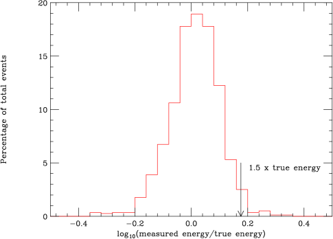
Figure 22: The AGASA energy resolution for showers of 10²⁰ eV.

The errors in energy reconstruction are calculated by simulation, where all the input is based on extensive experimental measurements. The resolution is presented in logarithmic units which is natural for the typical scale of errors in cosmic ray experiments. The natural unit here is 0.1. In Figure 22 we reproduce the plot of the expected energy fluctuation for showers of 10²⁰ eV for the AGASA experiment. The curve is asymmetric with a tail on the low energy side. The full width at half maximum (FWHM) is 0.2 corresponding to an RMS error of $\pm$ 21$\%$. More important is that probability of an upward fluctuation to $\geq$ 1.5 times the true energy is 2.8$\%$. Figures for showers of 3 x 10¹⁹ eV are 0.25 FWHM and 2.3$\%$ for an upward fluctuation beyond 1.5. With this resolution a GZK cutoff cannot be transformed into an excess of post-GZK events.

4.2 HiRes

The HiRes experiment is an extension of the original pioneering Fly’s Eye experiment [20]. The technique is to observe the yield of 300-400 nanometer photons produced by the fluorescence of charged particles passing through the nitrogen of the atmosphere. The fluorescence yield per unit track length is isotropic and roughly independent of the atmospheric pressure. One would expect the fluorescence emission to be proportional to dE/dx which would produce more photons per unit track length at higher pressure. The competition between deexcitation by collisions which increases with pressure and radiation deexcitation produces a fluorescence yield per unit track length that is nearly independent of pressure. The technique measures most directly the number of charged particles as the shower develops longitudinally. To get the corresponding energy deposit, one needs to know the density of the atmosphere corresponding the point in the sky where the fluorescence light is emitted. Thus, it is crucial to know independently the density of the atmosphere as a function of altitude. It is said that the fluorescence technique is “calorimetric”, but a purist might disagree.

The HiRes experiment presently operating consists of two stations separated by 12.6 km. One station (HiRes I) has 21 mirrors with a view of the sky of 360^∘ in azimuth and 3^∘ to 17^∘ in elevation. The second station (HiRes II) has a view of 360^∘ in azimuth and 3^∘ to 31^∘ in elevation. The sky is divided into pixels of 1^∘ by 1^∘ by clusters of photomultipliers at the focus of each 3.8 m² mirror.

Figure 23: Sketch for the purpose of calculating the fluorescence yield. The indicated coordinates are proportional to distance

Figure 24: The spectrum of nitrogen fluorescence light. The abcissa is the wavelength in nanometers. The ordinate is the relative intensity.

In Figure 23 we present the geometry for the calculation of the fluorescence light produced by a shower. The axis of the shower and the position of the detector define the shower-detector plane. To a good approximation the light can be assumed to be emitted from a line source. In an element of length $\Delta$$s$, $N_{e}$ charged particles will emit $\eta$$N_{e}$ photons in the range 300-400 nm, where $\eta$ is the fluorescence yield per charged particle per meter. The fluorescence spectrum is shown in Figure 24. This is the spectrum measured by Bunner [21]. The distance from the line element to the fluorescence detector is $r$. The perpendicular distance from the shower axis to the detector is $r_{p}$. The number of photoelectrons received at the detector is given by:

$$p_{e}=\left[(\Delta s\eta)\epsilon\left(\frac{A}{4\pi r^{2}}\right)\delta\right]N_{e}.$$

Here $A$ is the area of the light collecting mirror in m², $\epsilon$ is the product of the reflectivity of the mirror, the transmission coefficient of the near UV filter normally used and the photocathode efficiency, $\eta$ is the fluorescence yield in photons/meter, and $\delta$ is the transmission of the fluorescence light over the distance r. With the auxiliary relations $\Delta$$s$ = $r$$\Delta$$\theta$/cos($\theta$) and $r$ = $r_{p}$/cos($\theta$) one finds yield of photoelectrons to be:

$$\frac{p_{e}}{A}=\frac{\eta\epsilon\Delta\theta}{4\pi}\frac{\delta}{r_{p}}N_{e}.$$

It is instructive to put in some numbers. Roughly $\eta$ $\sim$ 4.5 UV photons/meter and $\epsilon$ $\sim$ 0.16. Taking $\Delta$ $\theta$ = 0.0174 (1^∘) one finds:

$$\frac{p_{e}}{m^{2}deg}\sim 10^{-6}\frac{\delta}{r_{p}}N_{e},$$

where $r_{p}$ is expressed in kilometers.

Typically at the shower maximum there are about 7 x 10⁹ charged particles for a shower of 10¹⁹ eV. Typical attenuation lengths are about 10 km. Thus one expects for r_p = 20 km a fluorescence signal of about 50 p_e/m² for a pixel of 1 degree². Note that $\delta$ is not a constant but depends on the atmospheric transmission between the shower axis and the detector for each pixel.

The number of photoelectrons per square meter of mirror area and per degree of trajectory in the sky, recorded at the entrance of the detector, is a good place to match the sensitivity of the fluorescence detector to the external quantities, which are the geometry of the shower and the attenuation of the atmosphere. The absolute calibration of the fluorescence detector is a delicate matter and we will not go into the details here [22].

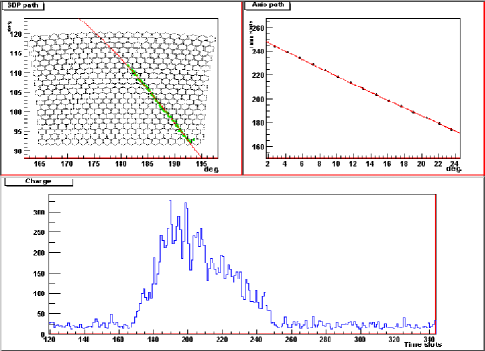
Figure 25: Example of the measurements made on a shower by a fluorescence detector.

As the shower develops Cherenkov light is produced. The number of Cherenkov photons is much greater than the number of fluorescence photons, but the former are very closely collimated along the shower axis. Nevertheless significant Cherenkov light can accompany the fluorescence signal. If the shower axis is directed at angles less than 30^∘ to the the fluorescence telescope axis, direct Cherenkov light will be detected. As the shower develops, the Cherenkov light accumulates along the shower axis, and this light is scattered into the field of view of the fluorescence telescope. There is also the night sky background which is ever-present. The night sky background is typically 40 photons per m² per $\mu$sec per deg² of sky. With a mirror area of 3.8 m² the mean night sky rate is roughly 23 p_e per $\mu$sec for each pixel. The Poisson fluctuations of this background rate modulate the fluorescence signal.

The measurements made by a fluorescence detector are shown in Figure 25. These are data from one of the Auger detectors, but are typical of the HiRes detector as well. In the upper left panel is the trace of the shower trajectory on the focal plane of the mirror. This information combined with the pointing direction of each pixel is used to construct the shower detector plane (SDP). The normal to this plane can be determined to an accuracy of a few tenths of a degree. In general the SDP can be strongly tilted with respect to the ground. In these cases the angular sweep of the fluorescence light can be much larger than the elevation aperture of the telescope. In the upper right panel is a plot of the time of arrival of the light in each pixel vs its angle $\chi_{i}$. These are the data needed to determine the location of the shower axis within the SDP. The lower panel is a plot of the light observed as a function of time in bins of 100 nsec (a FADC at 10 MHz). The night sky noise and the pedestals are evident before and after the fluorescence signal.

Figure 26: Plot of a true shower axis and two other shower axes that can also fit the angle-time data. The ambiguity is resolved by measurement of the time of arrival of the shower front on the ground (see discussion of hybrid method in text). If the axis were closer to the eye, the shower front would need to be delayed (not yet at ground level) since the light takes less time to get from the axis to the eye. Supposing the axis to be further from the eye would require the shower front to arrive ahead of the true front.

The angular velocity of the image of a vertical shower across the fluorescence camera is roughly about 1^∘/$\mu$sec at a distance of 20 km. It can be much faster if the shower is aimed towards the fluoresence telescope and much slower if it is aimed away from the telescope. HiRes I collects the signal from each pixel with sample-and-hold electronics with $\sim$ 5$\mu$sec integration time. HiRes II collects the signal with a 10 MHz FADC.

The location of the shower axis within the SDP is much less well determined and depends on the relative time of arrival of the fluorescence signals as a function of pixel angle. An individual skilled in trigonometry can show from Figure 23 that:

$$t_{i}-t_{0}=\frac{r_{p}}{c}tan\left(\frac{\pi-\psi-\chi_{i}}{2}\right),$$

where $t_{i}$ is the arrival time of the fluorescence light at the $i$th pixel at the angle $\chi_{i}$, $t_{0}$ is the time of emission of light at the point defined by r_p, and $c$, the velocity of light. The quantities $\psi$ and $r_{p}$ define the position and angle of the shower axis in the SDP and hence the shower geometry is completely determined. The angle $\pi-\psi-\chi$ is the angle between the shower axis and the trajectory of the light ray to the detector. For short segments and/or segments roughly perpendicular to the direction of observation, many combinations of $r_{p}$ and $\psi$ can satisfy the angle-time relation. An example of this for a SDP perpendicular to the ground is shown in Figure 26. The true shower axis is the solid one, but axes at $\pm$ 10^∘ to the true one produce only a slightly different angle time relation. Information that breaks the degeneracy of many possible sets of $\psi$ and $r_{p}$ depends on a measurable curvature in the angle time relation. For the example shown in Figure 26 the sagittas (a measure of curvature) deviate by only $\pm 0.4\mu$sec for the dashed trajectories. Consequently a single fluorescence detector (monocular) has a very asymmetric angular resolution.

Figure 27: Ratio of energy by monocular reconstruction to energy by hybrid reconstruction for showers observed in the hybrid mode by the Auger Observatory. The energy of the showers is between 10¹⁸ and 10¹⁹ eV.

The conversion of the observed light pattern in the FADC to number of particles as a function of atmospheric depth in gm/cm² depends on the zenith angle of the shower axis and a knowledge of the density of the atmosphere as a function of height. A poor measurement of the angle $\psi$ and $r_{p}$ will result in a poor energy measurement. To avoid this problem the original Fly’s Eye experiment [23] and the HiRes experiment chose to view the showers in stereo. Then the intersection of the two SDPs gives an accurate measure of the shower axis.

A second method which requires only a single fluorescence telescope uses the measurement of the relative time of arrival of the fluorescence light with the time of arrival of shower particles in one or more surface detectors. As shown in Figure 26, a measurement of the arrival time of the shower particles selects the true trajectory. This hybrid technique [24] is employed by the Auger Observatory. The precision is as good or better than a stereo arrangement.

The Auger Observatory with a small number of surface detectors was operated for a few months in a hybrid mode. A coincidence between a fluorescence detector and even a single surface detector gives a precision for the intersection of the shower axis with the ground of better than 100 meters. In Figure 27 we show the ratio of the energy by mono reconstruction to hybrid reconstruction which is a measure of the accuracy of the mono reconstruction. While the circumstances are not exactly the same as with HiRes, one gains some appreciation for the accuracy of a mono analysis which is not so bad ($\pm$ 25$\%$).

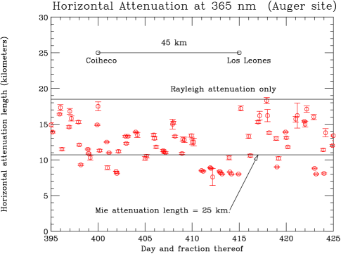
Figure 28: The horizontal attenuation length at the Auger Observatory site, 1400 meters elevation.

The FADC light trace in Figure 25 must be converted to the number of charged particles as a function of atmospheric depth. This conversion involves correction for the attenuation in the atmosphere. There are two components to this correction, the Rayleigh scattering in the air, and the scattering of by aerosols in the air (Mie scattering). The latter can be highly variable and must be measured. If the vertical structure of the atmosphere is known, the effects of Rayleigh scattering can be evaluated. A discussion of these most important corrections are beyond the scope of this article. A very clear discussion of the atmospheric corrections can be found in the reference [25]. While this paper refers to the atmospheric monitoring program of the Auger Observatory, it shares many of the features of the HiRes program and has greatly benefited from collaboration with the HiRes group. The Rayleigh attenuation length at the elevation of the HiRes site is $\sim$18 km. It lengthens with altitude as the density of the atmosphere decreases as e^-(h/7.5) where h is the altitude in km. Typical values of the aerosol absorption length are about 25 km, but are highly variable. The scale height for the aerosols is usually much smaller than the atmosphere being, $\sim$ 1.2 km. For proper correction extensive atmospheric monitoring is employed using LIDAR and horizontal attenuation monitors. The horizontal attenuation length of the atmosphere at the detector level shows in dramatic fashion the variation of the atmosphere. The horizontal attenuation length at the Auger site is plotted for a month period in Figure 28. There are occasions where the attenuation length shows the complete absence of aerosols.

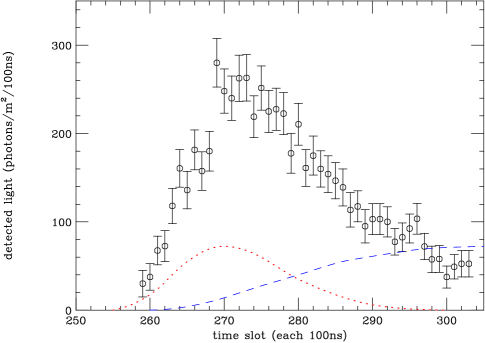
Figure 29: A typical light curve vs time measured by one of the Auger fluorescence telescopes. The points with errors are the observed photons/m²/100ns entering the telescope. Shown is the total signal and the contributions to it by Cherenkov light. The direction of this shower was chosen to show both direct Cherenkov light (dots) and scattered Cherenkov light (dashes).

The current analysis of the HiRes data has been made with average values for the aerosol scattering and the aerosol scale height. This procedure is sufficient for analysis at no better than a 25$\%$ level. The ultimate analysis will certainly take into account the variability of the atmosphere. Typical attenuation lengths are about 15 km. At 20 km this corresponds to a correction of a factor 4 and at 30 km a factor 7. As the highest-energy events require the largest aperture, they will be the most distant and will require the largest correction. The attenuation correction is of course not a single number, but depends on the geometrical path of the light to each pixel. The depth of shower maximum of the light curve depends on the attenuation correction. Finer details can be imagined. The fluorescence yield consists of discrete bands ranging from 310 to 390 nm. The Rayleigh attenuation length, which varies as $\lambda^{4}$, changes by nearly a factor of 5 over this range. Thus, it is important to know not only the overall fluorescence yield but, also its individual components very accurately.

A typical light curve observed by an Auger fluorescence telescope is shown in Figure 29. The light curve is a mixture of fluorescence light and Cherenkov light. In this particular case there are contributions for both direct Cherenkov light which contaminates the early part of the light curve and scattered Cherenkov light which is important near the tail of the signal. An iterative technique is used as the strength of the Cherenkov signal depends on the $N_{e}$ which is derived from the fluorescence signal itself. The geometry of the shower axis with respect to the telescope must be reconstructed to determine the Cherenkov subtraction. The energy is determined from the ionization loss of the charged particles. In addition some 5 to 10$\%$ of energy is not visible due to muons and neutrinos.

The fluorescence technique is a very beautiful one. However it needs enormous attention to details to exploit its ultimate precision. These details include absolute calibration of the optical system, gain monitoring, atmospheric monitoring, absolute knowledge of the nitrogen fluorescence efficiency, and the vertical profile of the atmosphere which varies between summer and winter. The detector can only operate on dark moonless nights which limits its duty cycle to $\sim 10\%$. The viewing time is longer in the winter. Many years are required to achieve uniform exposure in right ascension. The surface array is robust and can operate in all weather with $\sim 100\%$ duty cycle. Nature provides a constant calibration in the form of an abundance of single cosmic ray muons. However without an independent means of calibration simulations are required to establish the energy scale.

In metaphorical terms the fluorescence technique resembles a beautiful prima donna who needs constant pampering. Then she will sing with such beauty that shivers run up and down your spine. By contrast the surface array technique reminds one of a chanteuse in a smoky bar who sings with the same passion, no matter how she feels or how she is treated.

5 Experimental results

5.1 Energy spectrum

The HiRes and AGASA detectors are located at approximately the same latitude, 40.3^∘N and 35.5^∘N respectively. Thus they look at the same region of sky and are expected to observe the same spectrum of cosmic rays. This would not necessarily be the case for a comparison with a spectrum from the southern hemisphere. The data presented by the AGASA array has been accumulated over 12 years [18]. Their analysis is very mature and they have responded in detail to to a number of thoughtful criticisms [17]. In this paper the AGASA group estimates the systematic error of their energy measurement to be $\pm$ 18$\%$. The aperture of AGASA is flat above 10¹⁹ eV as its calculation is insensitive to the exact details of the trigger since many detectors are hit. The aperture decreases as the energy drops below 10¹⁹ eV. The efficiency to record a shower then depends on the position of the shower on the array and the criteria for a scintillator to trigger. The calculation of the aperture is critical in the conversion of the number of events per energy bin to a flux. When the array is not fully efficient this calculation is sensitive to precise understanding of the individual detector and the details of the lateral distribution.

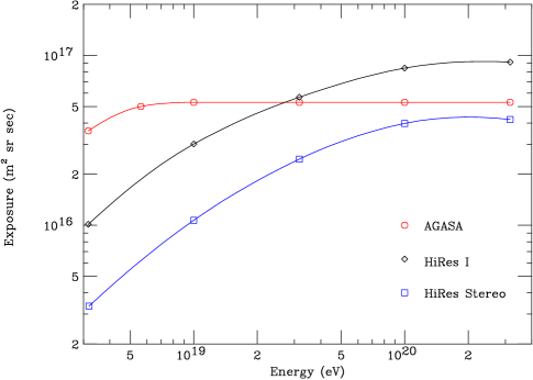
Figure 30: The exposure of the AGASA experiment, the HiRes I monocular experiment, and the HiRes stereo experiment as reported at the 2003 ICRC.

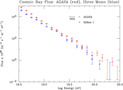
Figure 31: Plot of the AGASA spectrum (circles) and the HiRes I monocular spectrum (squares) for energies $\geq 10^{18.5}$.

Recently the HiRes group has reported on 5.7 years of monocular operation from HiRes I [26] with 2820 hours of data. (Periods of lack access to the Dugway site certainly reduced the amount of data that potentially was available.) The group has also reported 1006 hours of stereo data which is intrinsically more reliable [27].

As HiRes I has an elevation coverage from only 3^∘ to 17^∘ an extra constraint was required to reconstruct these mono events. They constrained the traces to fit a Gaisser-Hillas profile with an X_max between 680 and 900 gm/cm² to supplement the angle-time reconstruction of the shower axis in the SDP. They estimate the RMS energy resolution to be better than 20$\%$ above 3x10¹⁹ eV. The data are analysed with average values for the atmospheric conditions. It is intrinsic to the fluorescence technique that the aperture grows with energy. A higher-energy shower can be seen further away. So at all energies the calculation of the aperture depends on many details. The authors estimate that the total systematic error in their energy measurement is 21$\%$. A separate estimate of the systematic error in the aperture is not clearly given. The interest in this spectrum is that at 10²⁰ eV its exposure exceeds that of AGASA. The exposures for the three measurements are plotted as a function of energy in Figure 30. The spectra for HiRes I and AGASA are plotted in Figure 31. The two spectra in the energy range from 10¹⁹eV to 10²⁰ eV show remarkable agreement considering an estimated systematic error of about 20$\%$ for each experiment. A shift in energy of one or the other experiment by $25\%$ will produce good agreement. Much has been made of the absence of events beyond 10²⁰ eV in the HiRes I data, notably by authors whose theories on the origins of the highest-energy cosmic rays predict a GZK cutoff [28]. I have a few comments to offer. First, the more reliable HiRes stereo data will give a far more convincing case if the absence of events beyond 10²⁰ eV is to be confirmed. In addition to significantly more stereo exposure, one expects many improvements in the analysis. Also one cannot easily make the 11 AGASA events above 10²⁰ eV go away, and they are too many to be explained as resolution spillover. Further, as explained in the propagation part of this paper, the fluctuations in the events found above the GZK cutoff can be very large.

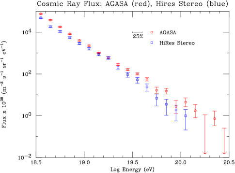
Figure 32: The HiRes stereo spectrum as presented at the 2003 ICRC.

The HiRes stereo spectrum has been eagerly anticipated. Its exposure does not yet match that of AGASA. And the analysis has not yet reached a maturity that one can ultimately expect. The average atmosphere must be replaced by the nightly measurements and improvements must be made in the energy calibration and the aperture calculation. The experiment continues to run and ultimately it can provide the best measurements in the northern hemisphere for some time to come. The stereo spectrum as reported at the 2003 ICRC is shown in Figure 32. For comparison the AGASA spectrum is replotted. The amount of HiRes stereo data in this plot is $\sim$ 25$\%$ of what will eventually be available.

5.2 Anisotropy and cluster analysis

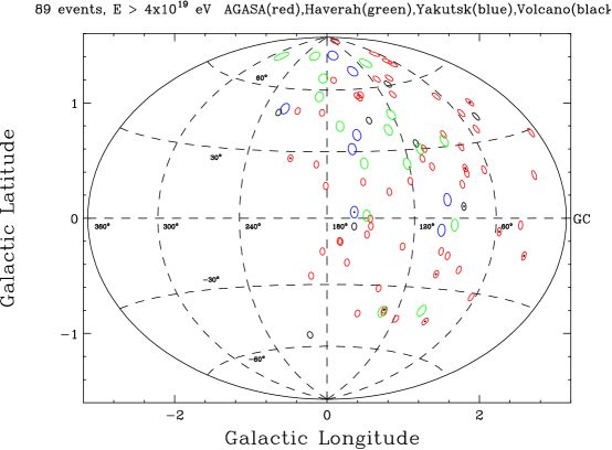
Figure 33: Arrival directions of cosmic rays with energy $\geq$ 4 x 10¹⁹ eV observed by AGASA, Haverah Park, Yakutsk, and Volcano Ranch. The size of the oval boundary represents the angular resolution. A dot within the oval indicates that the cosmic ray had an energy $\geq$ 10²⁰eV. The small ovals come from AGASA or Volcano Ranch. The larger ovals come from Yakutsk or Haverah Park.

The distribution of directions for cosmic rays in the northern hemisphere is plotted in galactic coordinates in Figure 33. The choice of minimum energy is 4 x 10¹⁹ eV. This energy was chosen by the AGASA group to make their cluster analysis. The rationale for this choice is not clear, perhaps a balance between a sufficiently high energy so that the selected events have some chance to point to a source and the desire to have a reasonable number of events. There are a total of 89 events plotted, 57 events from AGASA [29], 16 from Haverah Park [30], 8 from Yakutsk [31], and 8 from Volcano Ranch [32]. I regret that the $\sim$ 20 events from the HiRes stereo experiment were not available.

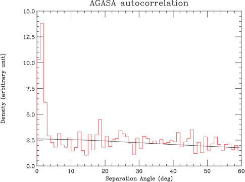
Figure 34: Distribution of angular distances between pairs of 59 AGASA events with energy $\geq$ 4 x 10¹⁹ eV weighted by the inverse of the solid angle of the angular bin. The solid line is the distribution expected for random arrival directions.

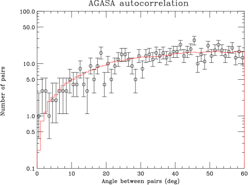
Figure 35: Distribution of angular distances between pairs of 57 AGASA events with energy $\geq$ 4 x 10¹⁹ eV. The histogram is the distribution expected for random arrival directions. The errors represent 68$\%$ confidence limits.

The distribution of the cosmic ray directions in the northern sky shows no gross anisotropy. There are 4 pairs and one triplet in the sample of AGASA events with energy $\geq$ 4 x 10¹⁹ eV. The pairs or triplet are defined as two or three events whose angular separation is less than 2.5^∘ This analysis is based on data collected through May 2000 when the AGASA exposure was 4.0 x 10¹⁶ m² sr sec. No public catalog of directions has been published for more recent data although the AGASA spectrum discused above is based on data accumulated through December 2002 [18]. The AGASA experiment was terminated on Jan 4, 2004 and will have accumulated a total exposure of $\sim$ 6.0 x 10¹⁶ m² sr sec. So we can expect at least 50$\%$ more events when the cluster analysis is complete. Figure 34, which appears in [29], is a plot of the separation angles between all pairs of cosmic rays in angular bins of 1^∘. Each bin is weighted by the inverse of the solid angle of that bin. There were eight pairs contributing to the plot, three of which are part of a triplet. However to make the eighth pair the limit of 4 x 10¹⁹ eV was lowered to 3.89 x 10¹⁹ eV to pick up an additional pair. The distribution of angles for random directions in the sky was generated from the data itself by choosing the right ascension of each event randomly between 0 and 360^∘. This procedure was repeated for the data set many times and the resulting average distribution of angles between pairs is plotted as the solid line. An impressive peak results at small angles but one has no sense of its significance as no errors are indicated.

I have made a plot of the pair angle distribution not weighted by the inverse of the solid angle which is shown in Figure 35. This plot includes the 57 events from the AGASA catalog, not pulling in the eighth pair. Here the observed number of events is plotted along with a histogram of the distribution expected for a random right ascension. For each point the 68$\%$ confidence limits are plotted [33]. The information to assess the significance is now revealed. For the first three bins 7 pairs are observed where 2.2 are expected. The Poisson probability to observe 7 or more pairs is .0075. I will leave it to experts to evaluate the true significance, but as experience shows, this evidence for pairs is not yet convincing. I have made a similar analysis for pairs using the 89 events in the skymap of Figure 33. Here for the first three bins there are 12 pairs with an expected 6.0 for the randomized distribution. For this case the probability to observe 12 or more pairs is .02.

The most striking aspect of the Figure 33 is the appearance of a second triplet. I have made an analysis similar to the pair analysis described above. The equivalent of the angle between pairs was the average of the three angles between the members of a triplet. Plotting this average angle for all possible triplets yielded two triplets within the first three angular bins just as seen by eye. Expected from the random distribution were 0.7 triplets. The Poisson probability for this case is 0.10.

There is no sense to try to squeeze more significance out of these data, but it is instructive to play a bit. It happens that, if the threshold is increased to 5 x 10¹⁹ eV, the triplets remain and all pairs except those contained in the triplets disappear. The number of events decreases from 89 to 53. If one repeats the triplet calculation, the Poisson probability to observe two or more triplets is 0.003.

One of the lessons is the obvious one that one needs more data. The other lesson is that one might raise the lower energy cut to enhance the likelihood that the events come from a distance of less than 100 Mpc. Reference to Figure 6 shows that 90$\%$ of the events with energy 8 x 10¹⁹ eV travel a distance of $\leq$ 100 Mpc. Thus, in searching for pairs, a lower limit of 8 x 10¹⁹eV might be a cut with some physical motivation behind it. Such a selection is beyond the reach of the presently operating experiments but may be within the reach of the Auger Observatory. However Auger in the southern hemisphere looks away from the Virgo cluster where there are significant concentrations of extragalactic matter which might serve as sources.

5.3 Composition

To measure the composition of the primary cosmic rays is the most difficult challenge of all, far more so than the energies and directions. One seeks to infer the nature of the primary particle from the 10¹⁰ secondaries produced. The two principal observables that can be traced to the nature of the primary are the depth of maximum of the shower (X_max) and the ratio of the muonic to to electromagnetic components of the shower. There are secondary observables related to these primary observables. For a given energy the showers are successively more penetrating (larger X_max) as one passes from a heavy primary to a proton to a photon. A deeper shower has a sharper lateral distribution (the shower has less distance to spread). The spread in time of shower particles that arrive at a detector far from the axis is larger for a deeply penetrating shower. In addition, the muon to electromagnetic ratio decreases as the shower is more penetrating. This ratio is roughly 40$\%$ lower for protons than for the heaviest nucleus expected in the cosmic rays. Photons at the highest energy $\geq$ 10¹⁹ eV have a muon to electromagnetic ratio more than a factor three less than protons.

In all the literature concerning composition one speaks of protons and iron as if these are the only possibilities. This is because these two primaries represent the extremes. There is barely the means to even separate iron and protons, so that any mixture of protons and nuclei can be fit in this two component model. A measurement of X_max is a quantity most directly related to composition. A measurement of this quantity as a function of energy is Linsley’s elongation rate. The bounds of the elongation rate must be calculated by simulation, and these can vary by 10’s of gm/cm² so the absolute position of X_max as a function if primary is quite uncertain. The slopes of the boundaries are less sensitive to the interaction models. A steepening or a flattening of the elongation rate indicates a change in composition towards a lighter or heavier mix of nuclei.

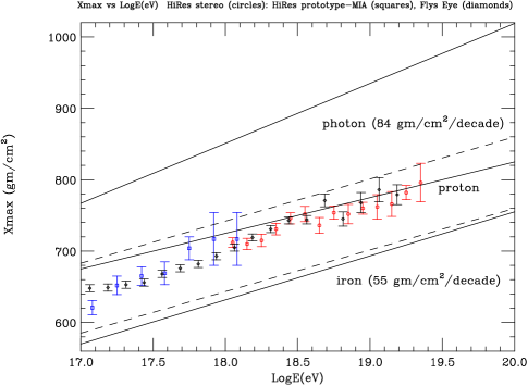
Figure 36: Plot of X_max vs energy measured by measurements of the Fly’s Eye and HiRes experiments. The boundaries indicated for iron and proton are based on the QGSJET interaction model (solid) and the Sibyll model (dashed). The elongation rate for photons is also plotted.

Additional composition information is contained in the fluctuation of X_max. In the section on shower properties we saw that the fluctuation for X_max for protons was 53 gm/cm², while for iron it was 22 gm/cm². The magnitude of these fluctuations is weakly dependent on the choice of interaction model.

The fluorescence detectors can measure X_max with a statistical error of $\leq$ 30 gm/cm². Recently the HiRes group presented a measurement of X_max in the range from 10¹⁸ eV to 2 x 10¹⁹ eV [34]. These results and prior measurements made with the HiRes prototype [35] and the original Fly’s Eye experiment [36] are plotted in Figure 36. Two different interaction models for the proton and iron boundaries are indicated. While the boundary differences are significant, it is amazing that the data do lie within the boundaries and the elongation rate for the different cases are about the same, 55 gm/cm² per decade.

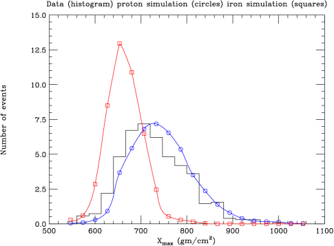
Figure 37: Distribution of values of X_max measured with the HiRes stereo detector. The data are represented by the histogram. The expected distribution for pure proton and pure iron are shown by the circles and squares respectively.

In Figure 36 the elongation rate for photon showers is also plotted. Above 10¹⁹ eV the curve strongly deviates from the indicated one because of interaction in the Earth’s geomagnetic field and the LPM effect. In either case the photon showers are much more deeply penetrating [37].

The interpretation of the data of Figure 36 is that the composition is moving towards a lighter mixture. However the conclusion of an extremely light mixture at 10¹⁹ eV or a heavier mixture depends on the choice of the interaction model. If the boundary comes from the Sibyll model, the composition is less proton rich than for the case of QGSJET.

Complementary information can be obtained from the fluctuations of X_max. The fluctuation of the HiRes stereo X_max measurements for all of the energies lumped together is plotted in Figure 37. It would have made more sense to divide the fluctuation distributions into separate energy bins so that the evolution from a heavier composition to a lighter composition could have been observed through the broadening of the fluctuation distribution. With the limited amount of data the HiRes group probably chose to combine all the data and any situation can be simulated. The data are compared with the QGSJET simulation for pure iron and pure proton. The shape of the X_max fluctuation is very suggestive of a proton rich composition. The danger is that, if the distribution is broadened by errors unaccounted for, there will be a bias towards a lighter composition. Nevertheless the relation between the width of the fluctuation distribution and the nuclear species is almost independent of the interaction model, and it represents the most promising measure of composition in the case where the errors in the X_max measurement have a negligible effect on the fluctuations.

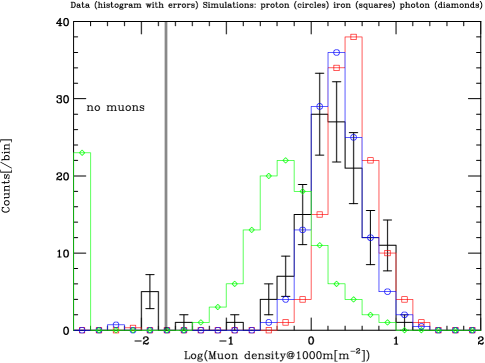
Figure 38: Plot of muon density at 1000m for showers with energy $\geq$10¹⁹ eV measured by the AGASA group. Black histogram with errors is the data, histograms marked with squares, circles, and diamonds are respectively the simulated distribution for iron, proton, and photon primaries respectively.

An alternative method for the measurement of composition depends on the muon content of the showers. All simulations show that showers produced by iron nuclei contain more muons than proton initiated showers. A typical ratio is 1.4. The AGASA array is outfitted with a number of muon detectors in the southern part of their array. In a fraction of the events above 10¹⁹ eV the density of muons at 1000m from the shower axis, $\rho_{\mu}$(1000), can be measured. The distribution for this quantity for iron, proton, and photon can be simulated. These results are shown in Figure 38. The individual measurements which each have a fractional RMS error of 40$\%$ scatter a great deal but their average is consistent with a proton rich mixture. Although this conclusion agrees with the HiRes stereo measurement it is much more model dependent. There is no evidence for a photon component and the upper limit for the photon fraction at 95$\%$ confidence is quoted as 34$\%$.

Analysis of the past Haverah Park data using modern simulation techniques has contributed significantly to the question of the composition [38]. Using the steepness of the lateral distribution, which is related to X_max, the Haverah Park group finds a proton fraction of $\sim$ 40$\%$ in the range of energy 3 x 10¹⁷ to 10¹⁸ eV. This result is consistent with the view that the composition becomes lighter as the energy increases from 10¹⁷ to 10¹⁹ eV. By comparing the rates of vertical and horizontal showers the Haverah Park group has shown that the photon fraction at 10¹⁹eV is less than 40$\%$ [39].

There is an unsubstantiated feeling by many that at the extreme energies the composition is proton rich. But at present the evidence is not very strong. As more HiRes stereo data become available with a well controled absolute energy calibration and with atmospheric attenuation corrections based on nightly measurements and not averages, the fluorescence method for composition determination can become the most reliable. In addition if in passing from 10¹⁷ eV to 10¹⁹ eV the composition moves from heavy to light, one must observe a narrow fluctuation distribution evolving into a broader one as theenergy increases.

6 Conclusions

I have attempted in this survey to explain without excessive complication the important aspects for the measurement of the properties of cosmic rays at the very highest energies ($\geq$ $10^{19}$ eV). There remain major uncertainties in all areas, spectrum, anisotropy, and composition. The AGASA experiment is now complete and one awaits the final catalog of events. It should be possible for the AGASA group to extend their published measurements to larger zenith angles. I eagerly await the additional data and improved analysis from the HiRes group.

I am also looking forward to see the new data which will come from the Pierre Auger Observatory, now under construction in the southern hemisphere. It is a hybrid detector which consists of both surface detectors and fluorescence telescopes. About 10$\%$ of showers will be observed simultaneously by both techniques. I will not list the advantages of the hybrid detector here; the reader can surely appreciate them. The curious reader is encouraged to visit the many web sites devoted to the Auger Observatory which can all be reached through www.auger.org. As I write these conclusions (February 2004) the Auger Observatory is operating with 220 surface detectors and 6 30^∘ x 30^∘ fluorescence telescopes. By the end of 2004 there will be 700-800 surface detectors and 12-14 fluorescence telescopes. By the end of 2005 it should be complete with 1600 surface detectors covering 3000 km² and 24 fluorescence telescopes overlooking the array.

The reader can surely appreciate the enormous gain in statistics and the detailed information that will be obtained for each event. However, from long experience in physics I succumb to caution and will refrain from making too many claims of what the Observatory will accomplish. Certainly we will learn a great deal. Pierre Auger made his great discovery 66 years ago. Nature rewarded John Linsley with a 10²⁰ eV shower 42 years ago. I hope that the many questions that these great discoveries have raised will be answered in a time much shorter than 42 or 66 years.

7 Acknowledgements

I am indebted to so many individuals over the years for contributing to my understanding of the highest-energy cosmic rays. A partial list includes Alan Watson, Michael Hillas, Tom Gaisser, M. Nagano, M. Teshima, Angela Olinto, Rene Ong, Johannes Knapp, Maria Teresa Dova, Pierre Billoir, Tokonatsu Yamamoto, Maximo Ave, Paul Sommers, Brian Fick, G. Sigl, Murat Boratav, Paul Mantsch, and Simon Swordy. I want to thank A. Watson, P. Sommers, K. Arisaka, and M. Dova for a critical reading of the manuscript but they are not responsible for any remaining errors.

This work was supported by the NSF grant PHY-0103717 and the Center for Cosmological Physics (NSF grant PHY-0114422).

References

- [1] M. Nagano, and A. A. Watson, Rev. Mod. Phys., 72, (2000), 689.
- [2] J. Linsley, Phys. Rev. Lett., 10, (1963), 146.
- [3] J. Linsley, 15th ICRC, Plovdiv, Bulgaria 12, (1977), 89.
- [4] A. M. Hillas, Ann. Rev. Astron. Astrophys., 22, (1984), 425.
- [5] K. Greisen, Phys. Rev. Lett., 16, (1966), 748; G. T. Zatsepin and V. A. Kuzmin, Sov. Phys. JETP Lett. (Engl. Transl.), 4, (1966), 78.
- [6] D. DeMarco, P. Blasi, and A. V. Olinto, astro-ph/0301497, to be published, Astropart. Phys.
- [7] T. E. Clarke, P. P. Kronberg, and H. Böhringer, astro-ph/0011281
- [8] P. P. Kronberg, Rep. Prog. Phys., 57, (1994), 325; P. Blasi, S. Burles, and A. V. Olinto, Ap. J., 514, (1999), L79.
- [9] These calculations are not intended to replace serious studies of propagation in magnetic fields given in the following references: O. Deligny, A. Letessier-Selvon, and E. Parizot, astro-ph/0303624; G. Sigl, M Lemoine, and P. Biermann, Astropart. Phys., 10, (1999), 141; C. Isola, M Lemoine, and G. Sigl, Phys. Rev. D, 65, (2002), 023004; T. Stanev, R. Engel, A. Mucke, R. J. Protheroe, and J. P Rauchen, Phys. Rev. D, 62, (2000), 093005; C. Isola and G. Sigl, Phys. Rev. D, 66, (2002), 083002; P. Blasi and A. V. Olinto, Phys. Rev. D, 59, (1999), 023001.
- [10] The two simulation programs that are being used are CORSIKA and AIRES. Information on CORSIKA can be found at www-ik3.fzk.de/heck/corsika/: information on AIRES can be found at www.fisica.unlp.edu.ar/auger/aires.
- [11] A comprehensive description of the Pierre Auger Observatory is given in Proceedings of the 27th ICRC, Hamburg, Germany, 2, (2001), 699-784.
- [12] M. Ave for the Pierre Auger Collaboration, astro-ph/0308523.
- [13] T. Gaisser and A. M. Hillas, Proceedings of the 15th ICRC, Plovdiv, Bulgaria, 8, (1977), 353
- [14] K. Shinozaki et al., Proc. 28th ICRC, Tokyo, (2003), 401, Universal Academy Press, Inc.
- [15] The Haverah Park array consisted of deep water tanks; see for example, M. A. Lawrence, R. J. O. Reid, and A. A. Watson, J. Phys. G17, (1991), 733.
- [16] Linsley was the first to observe the spread of arrival times as a function of distance from the shower axis: see J. Linsley and L. Scarsi, Phys. Rev., 128, (1962), 2384. Experiments performed before the advent of microelectronics recorded data with oscillocope photography and risetime information was available for the analysis. See for example, R. Walker and A. A. Watson, J. Phys G, 8, (1982), 1131.
- [17] M. Takeda et al., Astro. Part. Phys., 19, (2003), 499.
- [18] M. Takeda et al., Proc. 28th ICRC, Tokyo, (2003), 381, Universal Academy Press, Inc.
- [19] A. M. Hillas, D. J. Marsden, J. D. Hollows, and H. W. Hunter, Proc. 12th ICRC, Hobart, 3, (1971), 1001, University of Tasmania
- [20] D. Bird et al., Astrophys. J., 511, (1999), 739.
- [21] A. N. Bunner, Ph.D. thesis, Cornell University (1964); a copy of his plot is reproduced in R. M. Baltrusaitis et al., Nucl. Instrum. Methods Phys. Res. A, 240, (1985), 410. The most recent measurements of the total fluorescence yield are by, F. Kakimoto et al., Nucl. Instrum. Methods Phys. Res. A,372, (1996), 527, and M. Nagano, K. Kobayakawa, N. Sakaki, and K. Ando, Astropart. Phys., 20, (2003), 293.
- [22] J. A. J. Matthews, Proc. SPIE Conference on Astronomical Telescopes and Instrumention, (2002), Waikoloa, Hawaii; this paper describes the calibration of the Auger fluorescence telescope. The problems and techniques are common to both the Auger and HiRes detectors. A copy of this paper is also available as GAP-2002-029 from Technical Information at www.auger.org.
- [23] D. Bird et al., Nucl. Instrum. Methods Phys. Res. A, 349, (1994), 592.
- [24] P. Sommers, Astropart. Phys., 3, (1995), 349.
- [25] J. A. J. Matthews and R. Clay, Proc. 27th ICRC, Hamburg, Germany, 2, (2001), 745; also available as GAP-2001-029 from Technical Information at www.auger.org.
- [26] R. U. Abassi et al. for the The High Resolution Flys Eye Collaboration, astro-ph/0208243 v7 (2003); a brief version of this paper was presented at the 2003 ICRC; D. Bergman et al., Proc. 28th ICRC, Tokyo, (2003) 397, Universal Academy Press, Inc.
- [27] W. Springer et al., Proc. 28th ICRC, Tokyo, (2003), 409, Universal Academy Press, Inc; the HiRes stereo spectrum presented here is not contained in this paper but was presented at the conference.
- [28] J. N. Bahcall and E. Waxman, Phys. Lett., B556, (2003), 1.
- [29] M. Teshima et al., Proc. 28th ICRC, Tokyo, (2003), 437, Universal Academy Press, Inc. The catalog of the 57 events is given by N. Hayashida et al., astro-ph/0008102, (2000).
- [30] The Haverah Park directions were provided by A. A. Watson, private communication. Recently the Haverah Park energy scale was reduced by about 30 and that change has been roughly accounted for in the selection of events for Figure 33. see M. Ave et al. Proc 27th ICRC, Hamburg 1, (2001), 381.
- [31] The directions were provided by A. A. Mikhailov. I wish to thank Professor A. V. Glushkov for permission to use the Yakutsk directions and energies. The selection of Yakutsk events for Figure 33 were reduced by a factor log10=0.1 to better match the AGASA spectrum.
- [32] J. Linsley, Catalog of Highest Energy Cosmic Rays, edited by M. Wada (World Data Center of Cosmic Rays, Institute of Physical and Chemical Research, Itabashi, Tokyo) 1, (1980), 1.
- [33] The 68 limits were taken from the tables of R. D. Cousins and G. J. Feldman, Phys. Rev. D , 57, (1998), 3873.
- [34] G. Archbold and P. V. Sokolsky, for the HiRes collaboration. Proc. 28th ICRC, Tokyo, (2003), 405, Universal Academy Press, Inc.
- [35] T. Abu-Zayyad et al., Ap. J., 557, (2001), 686.
- [36] D. J. Bird et al., Phys. Rev. Lett., 71, (1993), 3401. The experimental points from the original Fly’s Eye experiment were raised by 20 gm/cm2 to compensate for a systematic experimental bias. This is described in T. K.Gaisser et al., Phys. Rev. D, 47, (1993), 1919. We quote from page 1925 of that paper: “ We estimate that the simulated showers can be shifted to a shallower Xmax to a maximum of about 20 gm/cm2, or alternatively the experimentally detected showers can be assigned Xmax deeper by the same amount.”
- [37] There are many papers on the interaction of photons with energy 1019 eV with the geomagnetic field and the LPM effect. A selection of these: T. Stanev and H. P. Vankov, Phys. Rev. D 55, (1997), 1365; X. Bertou, P. Billoir, and S. Dagoret-Campagne, Astropart. Phys., 14, (2000), 121; H. P. Vankov, N. Inoue, and K. Shinozaki, Phys. Rev. D, 67, (2003), 043002; P. Homola et al., astro-ph/0311442.
- [38] M. Ave et al., Astropart. Phys., 19, (2003), 61.
- [39] M. Ave et al., Phys. Rev. Lett., 85, (2000), 2244.