Frontier in Astroparticle Physics and Cosmology Invited Talk at the 6th RESCEU Symposium, Nov. 4-7 2003, Tokyo, Japan.

Frontier in Astroparticle Physics and Cosmology

Invited Talk at the 6th RESCEU Symposium, Nov. 4-7 2003, Tokyo, Japan.

Chapter 1 Brane-world cosmological perturbations

R. Maartens

MaartensR.

Abstract

Brane-world models provide a phenomenology that allows us to explore the cosmological consequences of some M theory ideas, and at the same time to use precision cosmology as a test of these ideas. In order to achieve this, we need to understand how brane-world gravity affects cosmological dynamics and perturbations. This introductory review describes the key features of cosmological perturbations in a brane-world universe.

1.1 Introduction

Despite the tremendous successes of the concordance model (based on general relativity and inflation), which can account for high-precision cosmological observations, there remain deep puzzles within this model. What is the fundamental theory underlying inflation (or providing an alternative that matches its successes)? What is the dark energy that appears to be dominating the energy density of the universe and driving its late-time acceleration, and how can it be explained by fundamental theory? What is the dark matter that dominates over baryonic matter? These unresolved questions at the core of the concordance model may be an indication that high-precision cosmology is probing the limits not only of particle physics, but also of general relativity. In any event, it is important to pursue the cosmological implications of quantum gravity theories – and at the same time to subject quantum gravity theories to the stringent tests following from high-precision data.

The fully quantum regime entails the break-up of the space-time continuum, but even when spacetime can be modelled as a continuum, significant corrections to general relativity will arise at energies below, but near, the fundamental scale. Traditionally, the fundamental scale has been thought to be the Planck scale, $M_{\rm p}\sim 10^{19}~{}$GeV. However, recent developments in M theory, a leading candidate quantum gravity theory [1], indicate that $M_{\rm p}$ may be an effective energy scale, with the true fundamental scale being lower [2]. A key aspect of M theory is the need for extra spatial dimensions. If there are $d$ extra (spatial) dimensions, with length scale $L$, then the true fundamental scale $M_{4+d}$ is given by

$$M_{\rm p}^{2}\sim M_{4+d}^{2+d}\,L^{d}\,.$$ (1.1)

If $L\gg M_{\rm p}^{-1}$, then $M_{4+d}\ll M_{\rm p}$. Experiments in colliders and table-top tests of gravitational force [3] imply the bounds $L\lesssim 0.1~{}$mm and $M_{4+d}\gtrsim 1~{}$TeV.

There are five distinct 1+9-dimensional superstring theories. In the mid-90 s duality transformations were found that relate these superstring theories and the 1+10-dimensional supergravity theory, leading to the conjecture that all of these theories arise as different limits of a single theory – M theory. The 11th dimension in M theory is related to the string coupling strength; the size of this dimension grows as the coupling becomes strong. At low energies, M theory can be approximated by 1+10-dimensional supergravity. It was also discovered that p-branes, which are extended objects of higher dimension than strings (1-branes), play a fundamental role in the (non-perturbative) theory. Of particular importance among p-branes are the D-branes, on which open strings can end. Roughly speaking, open strings, which describe the non-gravitational sector, are attached at their endpoints to branes, while the closed strings of the gravitational sector can move freely in the full spacetime (the “bulk”). Classically, this is realised via the localization of matter and radiation fields on the brane, with gravity propagating in the bulk (see Fig. 1).

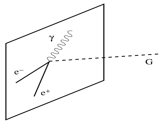
Figure 1.1: Brane-world schematic: matter is confined to the brane, while gravity propagates in the bulk (from [3]).

In the Horava-Witten solution [4], gauge fields of the standard model are confined on two 1+9-branes (or domain walls) located at the end points of an $S^{1}/Z_{2}$ orbifold, i.e., a circle folded on itself across a diameter. The 6 extra dimensions on the branes are compactified on a very small scale, close to the fundamental scale, and their effect on the dynamics is felt through “moduli” fields, i.e. 5D scalar fields. A 5D realization of the Horava-Witten theory and the corresponding brane-world cosmology is given in [5]. These solutions can be thought of as effectively 5-dimensional, with an extra dimension that can be large relative to the fundamental scale. They provide the basis for the Randall-Sundrum type 1 models of 5-dimensional gravity, with the bulk being a part of anti de Sitter spacetime (AdS₅) [6]. The scalar degree of freedom describing the inter-brane separation is known as the radion, and it requires a stabilization mechanism if general relativity is to be recovered at low energies.

As in the Horava-Witten solutions, the RS branes are $Z_{2}$-symmetric (mirror symmetry), and have tensions (vacuum energies) $\pm\sigma$, where

$$\sigma={3M_{\rm p}^{2}\over 4\pi\ell^{2}}\,.$$ (1.2)

Here $\ell$ is the curvature radius of the bulk, whose vacuum energy (cosmological constant) is

$$\Lambda_{5}=-{6\over\ell^{2}}\,.$$ (1.3)

The single-brane Randall-Sundrum type 2 models [7] with infinite extra dimension arise when the orbifold radius tends to infinity. In this case, general relativity is recovered at low energies; the weak-field gravitational potential is

$$\psi(r)={m\over r}\left(1+{2\ell^{2}\over 3r^{2}}\right)\,.$$ (1.4)

The fundamental scale is given by

$$M_{5}^{3}={M_{\rm p}^{2}\over\ell}\,.$$ (1.5)

1.2 The brane observer’s viewpoint

Extra dimensions lead to new scalar, vector and tensor degrees of freedom on the brane from the bulk graviton. In 5D, the spin-2 graviton is represented by a 4-transverse traceless metric perturbation. In a suitable gauge, this contains: a 3-transverse traceless perturbation – the 4D spin-2 graviton (2 polarizations); a 3-transverse vector perturbation – the 4D spin-1 gravi-vector (or gravi-photon) (2 polarizations); and a scalar perturbation – the 4D spin-0 gravi-scalar (1 polarization). These modes of the 5D graviton are massive from the brane viewpoint (essentially since the projection onto the brane of the null 5D momentum is a timelike momentum on the brane). They are known as Kaluza-Klein (KK) modes. The standard 4D graviton corresponds to the massless zero-mode of the spin-2 part. In RS1, the tower of massive modes is discrete, while in RS2 it is continuous.

The novel feature of the RS models compared to previous higher-dimensional models is that the observable 3 dimensions are protected from the large extra dimension (at low energies) by curvature rather than straightforward compactification. The RS brane-worlds and their generalizations (to include matter on the brane, scalar fields in the bulk, etc.) provide phenomenological models that reflect at least some of the features of M theory, and that bring exciting new geometric and particle physics ideas into play. The RS2 models also provide a framework for exploring holographic ideas that have emerged in M theory. Most of the recent progress on brane-world cosmology has been in RS-type models. (Recent reviews are given in [8, 9, 10]).

The field equations are [11]

$${}^{(5)}\!G_{AB} = -\Lambda_{5}\,^{(5)}\!g_{AB}\,,~{}(\mbox{bulk})$$ (1.6)

$$G_{\mu\nu} = -\Lambda g_{\mu\nu}+\kappa^{2}T_{\mu\nu}+6\frac{\kappa^{2}}{\sigma}{\cal S}_{\mu\nu}-{\cal E}_{\mu\nu}\,,~{}\mbox{(brane)}$$ (1.7)

where

$$\kappa^{2} \equiv \kappa^{2}_{4}={1\over 6}\sigma\kappa^{4}_{5}\,,$$ (1.8)

$$\Lambda \equiv \Lambda_{4}={1\over 2}\left[\Lambda_{5}+\kappa^{2}\sigma\right]\,,$$ (1.9)

and the standard 4D conservation equations hold on the brane (when there is only vacuum energy in the bulk):

$$\nabla^{\nu}T_{\mu\nu}=0\,.$$ (1.10)

The induced field equations (1.7) show two key modifications to the standard 4D Einstein field equations arising from extra-dimensional effects:

• ${\cal S}_{\mu\nu}\sim(T_{\mu\nu})^{2}$ is the high-energy correction term, which is negligible for $\rho\ll\sigma$, but dominant for $\rho\gg\sigma$:

  $${|\kappa^{2}{\cal S}_{\mu\nu}/\sigma|\over|\kappa^{2}T_{\mu\nu}|}\sim{|T_{\mu\nu}|\over\sigma}\sim{\rho\over\sigma}\,.$$ (1.11)

• ${\cal E}_{\mu\nu}$, the tracefree projection of the bulk Weyl tensor on the brane, encodes corrections from 5D graviton effects. These include the effects of the KK modes in the linearized case, and the gravitational influence of the second brane if there is one.

From the brane-observer viewpoint, the energy-momentum corrections in ${\cal S}_{\mu\nu}$ are local, whereas the KK corrections in ${\cal E}_{\mu\nu}$ are nonlocal, since they incorporate 5D gravity wave modes. These nonlocal corrections cannot be determined purely from data on the brane. They are constrained by the 4D contracted Bianchi identities ($\nabla^{\nu}G_{\mu\nu}=0$), applied to Eq. (1.7):

$$\nabla^{\mu}{\cal E}_{\mu\nu}={6\kappa^{2}\over\sigma}\,\nabla^{\mu}{\cal S}_{\mu\nu}\,.$$ (1.12)

This shows qualitatively how 1+3 spacetime variations in the matter-radiation on the brane can source KK modes. The 9 independent components in the tracefree ${\cal E}_{\mu\nu}$ are reduced to 5 degrees of freedom by Eq. (1.12); these arise from the 5 polarizations of the 5D graviton.

The trace free ${\cal E}_{\mu\nu}$ contributes an effective “dark” radiative energy-momentum on the brane, with energy density $\rho_{\cal E}$, pressure $\rho_{\cal E}/3$, momentum density $q^{\cal E}_{\mu}$ and anisotropic stress $\crossproduct_{\mu\nu}$:

$$-{1\over\kappa^{2}}{\cal E}_{\mu\nu}=\rho_{\cal E}\left({4\over 3}u_{\mu}u_{\nu}+{{1\over 3}}g_{\mu\nu}\right)+{q^{\cal E}_{\mu}}u_{\nu}+{q^{\cal E}_{\nu}}u_{\mu}+\crossproduct_{\mu\nu}\,.$$ (1.13)

We can think of this as a KK or Weyl “fluid”. The brane “feels” the bulk gravitational field through this effective fluid. The RS models have a Minkowski brane in an AdS₅ bulk. This bulk is also compatible with an FRW brane. However, the most general vacuum bulk with a Friedmann brane is Schwarzschild-anti de Sitter spacetime [12]. It follows from the FRW symmetries that $q^{\cal E}_{\mu}=0=\crossproduct_{\mu\nu}$, while $\rho_{\cal E}=0$ only if the mass of the black hole in the bulk is zero. The presence of the bulk black hole generates via Coulomb effects the dark radiation on the brane.

The brane-world corrections can conveniently be consolidated into an effective total energy density, pressure, momentum density and anisotropic stress. In the case of a perfect fluid (or minimally coupled scalar field),

$$\rho^{\text{tot}} = \rho\left(1+\frac{\rho}{2\sigma}+\frac{\rho_{\cal E}}{\rho}\right)\,,$$ (1.14)

$$p^{\text{tot }} = p+\frac{\rho}{2\sigma}(2p+\rho)+\frac{\rho_{\cal E}}{3}\;,$$ (1.15)

$$q^{\text{tot }}_{\mu} = q^{\cal E}_{\mu}\;,$$ (1.16)

$$\pi^{\text{tot }}_{\mu\nu} = \crossproduct_{\mu\nu}\;.$$ (1.17)

The (local) conservation equations (1.10) are

$$\dot{\rho}+\Theta(\rho+p)=0\,,$$ (1.18)

$$\nabla_{i}p+(\rho+p)A_{i}=0\,,$$ (1.19)

where $\Theta$ is the volume expansion rate ($=3H$ in FRW) and $A_{i}$ is the 4-acceleration. The nonlocal conservation equations (1.12) give [13]

$$\dot{\rho_{\cal E}}+{{4\over 3}}\Theta{\rho_{\cal E}}+\nabla^{i}q^{\cal E}_{i}=0\,,$$ (1.20)

$$\dot{q}^{\cal E}_{i}+{{4\over 3}}\Theta q^{\cal E}_{i}+{{1\over 3}}\nabla_{i}{\rho_{\cal E}}+{{4\over 3}}{\rho_{\cal E}}A_{i}+\nabla^{j}\crossproduct_{ij}=-{(\rho+p)\over\sigma}\nabla_{i}\rho\,,$$ (1.21)

where we have linearized about an FRW background.

1.3 The background cosmology

For an FRW brane, Eq. (1.21) is trivially satisfied, while Eq. (1.20) gives the dark radiation solution

$${\rho_{\cal E}}=\rho_{{\cal E}\,0}\left({a_{0}\over a}\right)^{4}\,.$$ (1.22)

In natural static coordinates, the Schwarzschild-AdS₅ metric for an FRW brane-world is

$${}^{\hat{\mathbf{d}}}s^{2} = -F(R)dT^{2}+{dR^{2}\over F(R)}+R^{2}\left({dr^{2}\over 1-Kr^{2}}+r^{2}d\Omega^{2}\right)\,,$$ (1.23)

$$F(R) = K-{C\over R^{2}}+{R^{2}\over\ell^{2}}\,,$$ (1.24)

where $K=0,\pm 1$ is the FRW curvature index and $C$ is the mass parameter of the black hole at $R=0$ (note that the 5D gravitational potential has $R^{-2}$ behaviour). The FRW brane moves radially along the 5th dimension, with $R=a(T)$, where $a$ is the FRW scale factor, and the junction conditions determine the velocity via the modified Friedmann equation (1.28). We can interpret the expansion of the universe as motion of the brane through the static bulk.

The velocity of the brane is coordinate-dependent, and can be set to zero. We can use Gaussian normal coordinates, in which the brane is fixed but the bulk metric is not manifestly static [14]:

$${}^{\hat{\mathbf{d}}}s^{2}=-N^{2}(t,y)dt^{2}+A^{2}(t,y)\left[{dr^{2}\over 1-Kr^{2}}+r^{2}d\Omega^{2}\right]+dy^{2}\,.$$ (1.25)

Here $a(t)=A(t,0)$ is the scale factor on the FRW brane at $y=0$, and $t$ may be chosen as proper time on the brane, so that $N(t,0)=1$. In the case where there is no bulk black hole ($C=0$), the metric functions are

$$N = {\dot{A}(t,y)\over\dot{a}(t)}\,,$$ (1.26)

$$A = a(t)\left[\cosh\left({y\over\ell}\right)-\left\{1+{\rho(t)\over\sigma}\right\}\sinh\left({|y|\over\ell}\right)\right]\,.$$ (1.27)

Again, the junction conditions determine the modified Friedmann equation [14]

$$H^{2}=\frac{\kappa^{2}}{3}\rho\left(1+{\rho\over 2\sigma}\right)+{C\over a^{4}}+\frac{1}{3}\Lambda-\frac{K}{a^{2}}\,,$$ (1.28)

and by Eq. (1.22),

$$C=\frac{\kappa^{2}}{3}\rho_{{\cal E}\,0}a_{0}^{4}\,.$$ (1.29)

The Friedmann and matter energy conservation equations yield

$$\dot{H}=-{\kappa^{2}\over 2}(\rho+p)\left(1+{\rho\over\sigma}\right)-2{C\over a^{4}}+{K\over a^{2}}\,.$$ (1.30)

The additional effective relativistic degree of freedom in dark radiation is constrained by nucleosynthesis and CMB observations to be no more than $\sim$5% of the radiation energy density [15, 16]:

$$\left.{\rho_{\cal E}\over\rho_{\rm rad}}\right|_{\rm nuc}\lesssim 0.05$$ (1.31)

The other modification to the Hubble rate is via the high-energy correction $\rho/\sigma$. In order to recover the observational successes of general relativity, the high-energy regime where significant deviations occur must take place before nucleosynthesis, i.e., cosmological observations impose the lower limit $\sigma>(1~{}{\rm MeV})^{4}$. This is much weaker than the limit from table-top experiments:

$$\ell<0.1~{}{\rm mm}~{}\Rightarrow~{}\sigma>(1~{}{\rm TeV})^{4}~{}{\rm and}~{}M_{5}>10^{5}~{}{\rm TeV}\,.$$ (1.32)

The background dynamics of brane-world cosmology are simple because the FRW symmetries simplify the bulk and rule out nonlocal effects. But perturbations on the brane in general release the nonlocal KK modes. Then the 5D bulk perturbation equations must be solved in order to solve for perturbations on the brane. These 5D equations are partial differential equations for the 3-Fourier modes, with complicated initial and boundary conditions.

The theory of gauge-invariant perturbations in brane-world cosmology has been extensively investigated and developed (see references given in the reviews [8, 9, 10]) and is qualitatively well understood. The key remaining task is integration of the coupled brane-bulk perturbation equations with appropriate initial/ boundary conditions. Special cases have been solved, where these equations effectively decouple, as in the next section, and approximation schemes have recently been developed [17, 18, 19, 20, 21] for the more general cases where the coupled system must be solved. From the brane viewpoint, the bulk effects, i.e., the high-energy corrections and the KK modes, act as source terms for the brane perturbation equations. At the same time, perturbations of matter on the brane can generate KK modes (i.e., emit 5D gravitons into the bulk) which propagate in the bulk and can subsequently interact with the brane. This nonlocal interaction amongst the perturbations is at the core of the complexity of the problem.

1.4 Brane-world inflation

In RS2-type brane-worlds, where the bulk has only a vacuum energy, inflation on the brane must be driven by a 4D scalar field $\phi$ trapped on the brane [22, 23]. (In more general brane-worlds, where the bulk contains a 5D scalar field, it is possible that the 5D field induces inflation on the brane via its effective projection [24]. More exotic possibilities arise from the interaction between two branes, including possible collision, which is mediated by a 5D scalar field and which can induce either inflation [25] or a hot big-bang radiation era, as in the “ekpyrotic” or cyclic scenario [26].)

High-energy brane-world modifications to the dynamics of inflation provide increased Hubble damping, since $\rho\gg\sigma$ implies $H$ is larger for a given energy than in 4D general relativity [22]. This makes slow-roll inflation possible even for potentials that would be too steep in standard cosmology [22, 27, 28].

The field satisfies the standard Klein-Gordon equation and the modified Friedmann equation, with $\rho={1\over 2}\dot{\phi}^{2}+V(\phi)$ and $p={1\over 2}\dot{\phi}^{2}-V(\phi)$. The condition for inflation is

$$\dot{\phi}^{2}-V+\left[{{1\over 2}\dot{\phi}^{2}+V\over\sigma}\left({5\over 4}\dot{\phi}^{2}-{1\over 2}V\right)\right]<0\,,$$ (1.33)

which reduces to the general relativity result, $\dot{\phi}^{2}<V$, when $\rho={1\over 2}\dot{\phi}^{2}+V\ll\sigma$. In the slow-roll approximation,

$$H^{2} \approx {\kappa^{2}\over 3}V\left[1+{V\over 2\sigma}\right]\,,$$ (1.34)

$$\dot{\phi} \approx -{V^{\prime}\over 3H}\,.$$ (1.35)

The brane-world correction term $V/\sigma$ in Eq. (1.34) serves to enhance the Hubble rate for a given potential energy, relative to general relativity. Thus there is enhanced Hubble ‘friction’ in Eq. (1.35), and brane-world effects will reinforce slow-roll at the same potential energy. We can see this by defining slow-roll parameters that reduce to the standard parameters in the low-energy limit:

$$\epsilon \equiv -{\dot{H}\over H^{2}}={M_{\rm p}^{2}\over 16\pi}\left({V^{\prime}\over V}\right)^{2}\left[{1+V/\sigma\over(1+V/2\sigma)^{2}}\right]\,,$$ (1.36)

$$\eta \equiv -{\ddot{\phi}\over H\dot{\phi}}={M_{\rm p}^{2}\over 8\pi}\left({V^{\prime\prime}\over V}\right)\left[{1\over 1+V/2\sigma}\right]\,.$$ (1.37)

Self-consistency of the slow-roll approximation then requires $\epsilon,|\eta|\ll 1$. At low energies, $V\ll\sigma$, the slow-roll parameters reduce to the standard form. However at high energies, $V\gg\sigma$, the extra contribution to the Hubble expansion helps damp the rolling of the scalar field and the new factors in square brackets become $\approx\sigma/V$:

$$\epsilon\approx\epsilon_{\rm gr}\left[{{4\sigma\over V}}\right]\,,~{}\eta\approx\eta_{\rm gr}\left[{{2\sigma\over V}}\right],$$ (1.38)

where $\epsilon_{\rm gr},\eta_{\rm gr}$ are the standard general relativity slow-roll parameters. In particular, this means that steep potentials which do not give inflation in general relativity, can inflate the brane-world at high energy and then naturally stop inflating when $V$ drops below $\sigma$. These models can be constrained because they typically end inflation in a kinetic-dominated regime and thus generate a blue spectrum of gravitational waves, which can disturb nucleosynthesis [27]. They also allow for the novel possibility that the inflaton could act as dark matter or quintessence at low energies [27, 29].

The key test of any modified gravity theory during inflation, will be the spectrum of perturbations produced due to quantum fluctuations of the fields about their homogeneous background values. In general, perturbations on the brane are coupled to bulk metric perturbations, and the problem is very complicated. However on large scales on the brane, the density and curvature perturbations decouple from the bulk metric perturbations [13, 22, 15] (see the next section). Thus we are justified in neglecting the bulk metric perturbations when computing the density perturbations.

To quantify the amplitude of scalar (density) perturbations we evaluate the usual gauge-invariant quantity

$$\zeta\equiv{\cal R}-{H\over\dot{\rho}}\delta\rho\,,$$ (1.39)

which reduces to the curvature perturbation, ${\cal R}$, on uniform density hypersurfaces ($\delta\rho=0$). This is conserved on large scales for purely adiabatic perturbations, as a consequence of energy conservation (independently of the field equations) [30]. The curvature perturbation on uniform density hypersurfaces is given in terms of the scalar field fluctuations on spatially flat hypersurfaces, $\delta\phi$, by

$$\zeta=H\,{\delta\phi\over\dot{\phi}}\,.$$ (1.40)

The field fluctuations at Hubble crossing ($k=aH$) in the slow-roll limit are given by $\langle\delta\phi^{2}\rangle\approx\left({H/2\pi}\right)^{2}$, a result for a massless field in de Sitter space that is also independent of the gravity theory [30]. For a single scalar field the perturbations are adiabatic and hence the curvature perturbation $\zeta$ can be related to the density perturbations when modes re-enter the Hubble scale during the matter dominated era, which is given by $A_{\rm s}^{2}=4\langle\zeta^{2}\rangle/25$. Using the slow-roll equations and Eq. (1.40), this gives

$$A_{\rm s}^{2}\approx\left.\left({512\pi\over 75M_{\rm p}^{6}}\,{V^{3}\over V^{\prime 2}}\right)\left[{2\sigma+V\over 2\sigma}\right]^{3}\right|_{k=aH}\,.$$ (1.41)

Thus the amplitude of scalar perturbations is increased relative to the standard result at a fixed value of $\phi$ for a given potential.

The scale-dependence of the perturbations is described by the spectral tilt

$$n_{\rm s}-1\equiv{d\ln A_{\rm s}^{2}\over d\ln k}\approx-6\epsilon+2\eta\,,$$ (1.42)

where the slow-roll parameters are given in Eqs. (1.36) and (1.37). Because these slow-roll parameters are both suppressed by an extra factor $\sigma/V$ at high energies, we see that the spectral index is driven towards the Harrison-Zel’dovich spectrum, $n_{\rm s}\to 1$, as $V/\sigma\to\infty$; however, this does not necessarily mean that the brane-world case is closer to scale-invariance than the general relativity case. In comparing the high-energy brane-world case to the standard 4D case, we implicitly require the same potential energy. However, precisely because of the high-energy effects, large-scale perturbations will be generated at different values of $V$ than in the standard case, specifically at lower values of $V$, closer to the reheating minimum. Thus there are two competing effects, and it turns out that the shape of the potential determines which is the dominant effect [31].

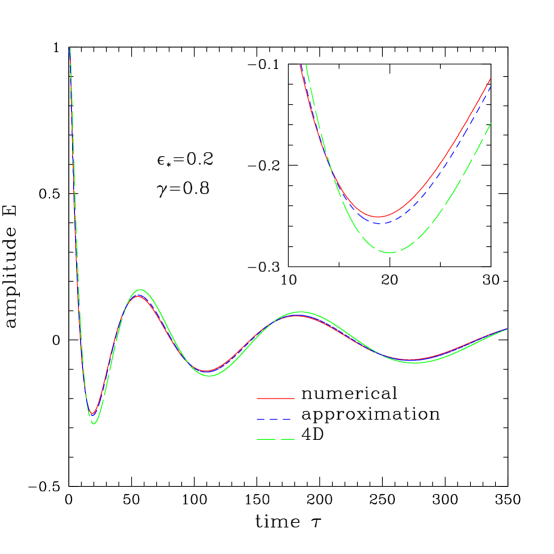
Figure 1.2: The damping of cosmological gravity waves on horizon re-entry due to massive mode generation. The solid curve is the numerical solution, the short-dashed curve the low-energy approximation, and the long-dashed curve the standard general relativity solution. $\epsilon_{*}=\rho_{0}/\sigma$ and $\gamma$ is a parameter giving the location of the regulator brane. (From [20].)

High-energy inflation on the brane also generates a zero-mode (4D graviton mode) of tensor perturbations, and stretches it to super-Hubble scales. This zero-mode has the same qualitative features as in general relativity, remaining frozen at constant amplitude while beyond the Hubble horizon. Its amplitude is enhanced at high energies, although the enhancement is much less than for scalar perturbations [32]:

$$A_{\rm t}^{2} \approx \left({32V\over 75M_{\rm p}^{2}}\right)\left[{3V^{2}\over 4\sigma^{2}}\right],$$ (1.43)

$${A_{\rm t}^{2}\over A_{\rm s}^{2}} \approx \left({M_{\rm p}^{2}\over 16\pi}\,{V^{\prime 2}\over V^{2}}\right)\left[{6\sigma\over V}\right].$$ (1.44)

Equation (1.44) means that brane-world effects suppress the large-scale tensor contribution to CMB anisotropies. The tensor spectral index at high energy has a smaller magnitude than in general relativity,

$$n_{\rm t}=-3\epsilon\,,$$ (1.45)

but remarkably the same consistency relation as in general relativity holds [28]:

$$n_{\rm t}=-2{A_{\rm t}^{2}\over A_{\rm s}^{2}}\,.$$ (1.46)

The massive KK modes of tensor perturbations of a de Sitter brane have a mass gap [33, 32, 34, 35]: $m>3H/2$. These massive modes remain in the vacuum state during slow-roll inflation [32, 34]. The evolution of the super-Hubble zero mode is the same as in general relativity, so that high-energy brane-world effects in the early universe serve only to rescale the amplitude. However, when the zero mode re-enters the Hubble horizon, massive KK modes can be excited, leading to a loss of energy from the zero mode, which can be estimated at low energies [20, 21] (see Fig. 2).

Vector perturbations in the bulk metric can support vector metric perturbations on the brane, even in the absence of matter perturbations [13]. However, there is no normalizable zero mode, and the massive KK modes stay in the vacuum state during brane-world inflation [36]. Therefore, as in general relativity, we can neglect vector perturbations in inflationary cosmology.

1.5 Curvature perturbations on large scales

The curvature perturbation ${\cal R}$ on uniform density surfaces is associated with the gauge-invariant quantity in Eq. (1.39). This is defined for matter on the brane, in the usual way. Similarly, for the Weyl “fluid” if $\rho_{\cal E}\neq 0$ in the background, the curvature perturbation on hypersurfaces of uniform dark energy density is

$$\zeta_{\cal E}={\cal R}+{\delta\rho_{\cal E}\over 4\rho_{\cal E}}\,.$$ (1.47)

On large scales, the dark energy conservation equation (1.20) implies

$$(\delta\rho_{\cal E})^{\displaystyle{\cdot}}+4H\delta\rho_{\cal E}+4\rho_{\cal E}\dot{\cal R}=0\,,$$ (1.48)

which leads to

$$\dot{\zeta}_{\cal E}=0\,.$$ (1.49)

For adiabatic matter perturbations, by the perturbed matter energy conservation equation,

$$(\delta\rho)^{\displaystyle{\cdot}}+3H(\delta\rho+\delta p)+3(\rho+p)\dot{\cal R}=0\,,$$ (1.50)

we find

$$\dot{\zeta}=0\,.$$ (1.51)

This is independent of brane-world modifications to the field equations, since it depends on energy conservation only. For the total, effective fluid, the curvature perturbation is defined as follows [15]: if $\rho_{\cal E}\neq 0$ in the background,

$${\zeta}^{\rm tot} = {\zeta}+\left[{4\rho_{\cal E}\over 3(\rho+p)(1+\rho/\sigma)+4\rho_{\cal E}}\right]\left(\zeta_{\cal E}-\zeta\right)\,,$$ (1.52)

and if $\rho_{\cal E}=0$ in the background,

$${\zeta}^{\rm\,tot} = {\zeta}+{\delta\rho_{\cal E}\over 3(\rho+p)(1+\rho/\sigma)}\,,$$ (1.53)

$$\delta\rho_{\cal E} = {\delta C\over a^{4}}\,,$$ (1.54)

where $\delta C$ is constant. It follows that the curvature perturbations on large scales can be found on the brane without solving for the bulk metric perturbations.

Although the density and curvature perturbations can be found on super-Hubble scales, the Sachs-Wolfe effect requires $\crossproduct_{\mu\nu}$ in order to translate from density/ curvature to metric perturbations. In the 4D longitudinal gauge of the metric perturbation formalism, the gauge-invariant curvature and metric perturbations on large scales are related by [15]

$$\zeta^{\rm tot} = {\cal R}-{H\over\dot{H}}\left({\dot{\cal R}\over H}-\psi\right)\,,$$ (1.55)

$${\cal R}+\psi = -\kappa^{2}a^{2}\delta\pi_{\cal E}\,,$$ (1.56)

where the radiation anisotropic stress on large scales is neglected, as in general relativity, and $\delta\pi_{\cal E}$ is the scalar potential for $\crossproduct_{\mu\nu}$. In 4D general relativity, the right hand side of Eq. (1.56) is zero. The (non-integrated) Sachs-Wolfe formula has the same form as in general relativity:

$${\delta T\over T}\Big{|}_{\rm now}=(\zeta_{\rm rad}+\psi-{\cal R})|_{\rm dec}\,.$$ (1.57)

The brane-world corrections to the general relativistic Sachs-Wolfe effect are then given by [15]

$${\delta T\over T}=\left({\delta T\over T}\right)_{\rm gr}-{8\over 3}\left({\rho_{\rm rad}\over\rho_{\rm cdm}}\right)S_{\cal E}-\kappa^{2}a^{2}\delta\pi_{\cal E}+{2\kappa^{2}\over a^{5/2}}\int da\,\,a^{7/2}\,\delta\pi_{\cal E}\,,$$ (1.58)

where $S_{\cal E}$ is the KK entropy perturbation (determined by $\delta\rho_{\cal E}$). The KK term $\delta\pi_{\cal E}$ cannot be determined by the 4D brane equations, so that $\delta T/T$ cannot be evaluated on large scales without solving the 5D equations. Equation (1.58) has been generalized to the 2-brane case, in which the radion makes a contribution to the Sachs-Wolfe effect [37].

The presence of the KK (Weyl, dark) component has essentially two possible effects.

• A contribution from the KK entropy perturbation $S_{\cal E}$ that is similar to an extra isocurvature contribution.

• A contribution from the KK anisotropic stress $\delta\pi_{\cal E}$. In the absence of anisotropic stresses, the curvature perturbation $\zeta^{\rm tot}$ would be sufficient to determine the metric perturbation ${\cal R}$ and hence the large-angle CMB anisotropies, via Eqs. (1.55), (1.56) and (1.57). However bulk gravitons can also generate anisotropic stresses which, although they do not affect the large-scale curvature perturbation $\zeta^{\rm tot}$, can affect the relation between $\zeta^{\rm tot}$, ${\cal R}$ and $\psi$, and hence can affect the CMB anisotropies at large angles.

1.6 Brane-world CMB anisotropies

Recently, the anisotropies in the CMB for RS-type brane-world cosmologies have been calculated using a low-energy approximation [18]. The basic idea of the low-energy approximation [17] is to use a gradient expansion to exploit the fact that, during most of the history of the universe, the curvature scale on the observable brane is much greater than the curvature scale of the bulk ($\ell<1~{}$mm):

$$L\sim|R_{\mu\nu\alpha\beta}|^{-1/2}\gg\ell\sim|\,^{\hat{\mathbf{R}}}_{ABCD}|^{-1/2}$$

$$\Rightarrow|\nabla_{\mu}|\sim L^{-1}\ll|\partial_{y}|\sim\ell^{-1}\,.$$ (1.59)

These conditions are equivalent to the low energy regime, since $\ell^{2}\propto\sigma^{-1}$ and $|R_{\mu\nu\alpha\beta}|\sim|T_{\mu\nu}|$:

$${\ell^{2}\over L^{2}}\sim{\rho\over\sigma}\ll 1\,.$$ (1.60)

Using Eq. (1.59) to neglect appropriate gradient terms in an expansion in $\ell^{2}/L^{2}$, the low-energy equation

$$\nabla^{\nu}{\cal E}_{\mu\nu}=0\,,$$ (1.61)

can be solved. However, two boundary conditions are needed to determine all functions of integration. This is achieved by introducing a second brane, as in the RS1 scenario. This brane is to be thought of either as a regulator brane, whose backreaction on the observable brane is neglected (which will only be true for a limited time), or as a shadow brane with physical fields, which have a gravitational effect on the observable brane.

The background is given by low-energy FRW branes with tensions $\pm\sigma$, proper times $t_{\pm}$, scale factors $a_{\pm}$, energy densities $\rho_{\pm}$ and pressures $p_{\pm}$, and dark radiation densities $\rho_{{\cal E}\,\pm}$. The physical distance between the branes is $\ell\bar{d}(t)$, and

$${d\over dt_{-}}=e^{\bar{d}}\,{d\over dt_{+}}\,,~{}a_{-}=a_{+}e^{-{\bar{d}}}\,,~{}H_{-}=e^{\bar{d}}\left(H_{+}-\dot{\bar{d}}\right)\,,~{}\rho_{{\cal E}\,-}=e^{4{\bar{d}}}\rho_{{\cal E}\,+}\,.$$ (1.62)

Then the background dynamics are given by

$$H_{\pm}^{2}=\pm{\kappa^{2}\over 3}\left(\rho_{\pm}\pm\rho_{{\cal E}\,\pm}\right)\,,$$ (1.63)

$$\ddot{\bar{d}}+3H_{+}\dot{\bar{d}}-\dot{{\bar{d}}}^{2}={\kappa^{2}\over 6}\left[\rho_{+}-3p_{+}+e^{2{\bar{d}}}(\rho_{-}-3p_{-})\right]\,.$$ (1.64)

The dark energy obeys $\rho_{{\cal E}\,+}=C/a_{+}^{4}$, where $C$ is a constant. From now on, we drop the +-subscripts which refer to the physical, observed quantities.

The perturbed metric on the observable (positive tension) brane is described, in longitudinal gauge, by the metric perturbations $\psi$ and ${\cal R}$, and the perturbed radion is $d={\bar{d}}+N$. The approximation for the KK (Weyl) energy-momentum tensor on the observable brane is [18]

$${\cal E}^{\mu}{}_{\nu} = \frac{2}{e^{2d}-1}\left[-\frac{\kappa^{2}}{2}\left(T^{\mu}_{\nu}+e^{-2d}T^{\mu}_{-~{}\nu}\right)\right.$$ (1.65)

$$\left.~{}~{}{}-\nabla^{\mu}\nabla_{\nu}d+\delta^{\mu}_{\nu}\nabla^{2}d-\left\{\nabla^{\mu}d\nabla_{\nu}d+\frac{1}{2}\delta^{\mu}_{\nu}(\nabla d)^{2}\right\}\right],$$

and the field equations on the observable brane can be written in scalar-tensor form as

$$G^{\mu}{}_{\nu} = \frac{\kappa^{2}}{\chi}T^{\mu}_{\nu}+\frac{\kappa^{2}(1-\chi)^{2}}{\chi}T^{\mu}_{-~{}\nu}$$ (1.66)

$$~{}{}+\frac{1}{\chi}\left(\nabla^{\mu}\nabla_{\nu}\chi-\delta^{\mu}_{\nu}\nabla^{2}\chi\right)+\frac{\omega(\chi)}{\chi^{2}}\left[\nabla^{\mu}\chi\nabla_{\nu}\chi-\frac{1}{2}\delta^{\mu}_{\nu}(\nabla\chi)^{2}\right],$$

where

$$\chi=1-e^{-2d}\,,~{}\omega(\chi)=\frac{3}{2}\frac{\chi}{1-\chi}\,.$$ (1.67)

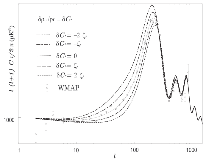
Figure 1.3: The CMB power spectrum with brane-world effects, for different values of the parameter $\delta C_{*}$ (which is the large-scale dark radiation fluctuation $\delta\rho_{\cal E}$ as a proportion of the large-scale curvature perturbation for matter $\zeta_{*}$). (From [18].)

The perturbation equations can then be derived as generalizations of the standard equations. The trace part of the perturbed field equation shows that the radion perturbation determines the crucial quantity, $\delta\pi_{\cal E}$:

$${\cal R}+\psi=-{2\over e^{2\bar{d}}-1}N=-\kappa^{2}a^{2}\delta\pi_{\cal E}\,,$$ (1.68)

where the last equality follows from Eq. (1.56). A new set of variables $\varphi_{\pm},E$ turns out be very useful [37, 18]:

$${\cal R} = -\varphi_{+}-{a^{2}\over k^{2}}H\dot{E}+\frac{1}{3}E\,,$$

$$\psi = -\varphi_{+}-{a^{2}\over k^{2}}(\ddot{E}+2H\dot{E})\,,$$

$$N = \varphi_{-}-\varphi_{+}-{a^{2}\over k^{2}}\dot{\bar{d}}\dot{E}\,.$$ (1.69)

The variable $E$ determines the metric shear anisotropy in the bulk, whereas $\varphi_{\pm}$ give the brane displacements, in transverse traceless gauge. The latter variables have a simple relation to the curvature perturbations on large scales [37, 18] (restoring the +-subscripts):

$$\zeta^{\rm tot}_{\pm}=-\varphi_{\pm}+{H_{\pm}^{2}\over\dot{H}_{\pm}}\left({\dot{\varphi}_{\pm}\over H_{\pm}}+\varphi_{\pm}\right)\,,$$ (1.70)

where $\dot{f}_{\pm}\equiv df_{\pm}/dt_{\pm}$.

The simplest model has

$$\rho_{\cal E}=0=\dot{\bar{d}}$$ (1.71)

in the background, with $p_{-}/\rho_{-}=p/\rho$. By Eq. (1.64), it follows that

$$\rho_{-}=-\rho e^{2\bar{d}}\,,$$ (1.72)

i.e., the matter on the regulator brane must have fine-tuned and negative energy density to prevent the regulator brane from moving in the background. The regulator brane is assumed to be very far from the physical brane, so that we can neglect its effects over a cosmological time-scale. With these assumptions, and further assuming adiabatic perturbations for the matter, there is only one independent brane-world parameter, i.e., the parameter measuring dark radiation fluctuations:

$$\delta C_{*}={\delta\rho_{\cal E}\over\rho_{\rm rad}}\,.$$ (1.73)

This has a remarkable consequence on large scales: the Weyl anisotropic stress $\delta\pi_{\cal E}$ terms in the Sachs-Wolfe formula Eq. (1.58) cancel the entropy perturbation from dark radiation fluctuations, so that there is no difference on the largest scales from the standard general relativity power spectrum. On small scales, beyond the first acoustic peak, the brane-world corrections are negligible. On scales up to the first acoustic peak, brane-world effects can be significant, changing the height and the location of the first peak. These features are apparent in Fig. 3. However, it is not clear to what extent these features are general brane-world features (within the low-energy approximation), and to what extent they are consequences of the simple assumptions imposed on the background. Further work remains to be done. (A related low-energy approximation, using the moduli space approximation, has been developed for certain 2-brane models with bulk scalar field [19].)

1.7 Conclusion

Simple brane-world cosmologies of RS type provide a rich phenomenology for exploring some of the ideas that are emerging from M theory. At the same time, brane-world gravity opens up exciting prospects for subjecting M theory ideas to the increasingly stringent tests provided by high-precision astronomical observations. Recent progress in tackling the massive KK modes for tensor and scalar perturbations, and in particular the development of an approximation scheme for computing CMB anisotropies, mean that these goals are brought closer to realization. On this basis, the perturbation analysis can be extended to cover more realistic brane-world models, and ultimately M theory models.

Acknowledgments

I thank the organisers for a very enjoyable and stimulating symposium. I am supported by PPARC.

Bibliography

- [1] For recent reviews, see, e.g., J.H. Schwarz, astro-ph/0304507; J. Polchinski, hep-th/0209105; R. Kallosh, hep-th/0205315.
- [2] N. Arkani-Hamed, S. Dimopoulos, G. Dvali, Phys. Lett. B429, 263 (1998) [hep-ph/9803315]; I. Antoniadis, N. Arkani-Hamed, S. Dimopoulos, G. Dvali, Phys. Lett. B436, 257 (1998) [hep-ph/9804398].
- [3] M. Cavaglia, Int. J. Mod. Phys. A18, 1843 (2003) [hep-ph/0210296].
- [4] P. Horava, E. Witten, Nucl. Phys. B460, 506 (1996) [hep-th/9510209].
- [5] A. Lukas, B.A. Ovrut, K.S. Stelle, D. Waldram, Phys. Rev. D59, 086001 (1999) [hep-th/9803235]; A. Lukas, B.A. Ovrut, D. Waldram, Phys. Rev. D60, 086001 (1999) [hep-th/9806022]; ibid., 61, 023506 (2000) [hep-th/9902071].
- [6] L. Randall, R. Sundrum, Phys. Rev. Lett. 83, 3370 (1999) [hep-ph/9905221].
- [7] L. Randall, R. Sundrum, Phys. Rev. Lett. 83, 4690 (1999) [hep-th/9906064].
- [8] R. Maartens, gr-qc/0312059.
- [9] P. Brax, C. van de Bruck, Class. Quantum Grav. 20, R201 (2003) [hep-th/0303095].
- [10] D. Langlois, astro-ph/0301021.
- [11] T. Shiromizu, K. Maeda, M. Sasaki, Phys. Rev. D62, 024012 (2000) [gr-qc/9910076].
- [12] S. Mukohyama, T. Shiromizu, K. Maeda, Phys. Rev. D62, 024028 (2000) [hep-th/9912287]; P. Bowcock, C. Charmousis, R. Gregory, Class. Quantum Grav. 17, 4745 (2000) [hep-th/0007177].
- [13] R. Maartens, Phys. Rev. D62, 084023 (2000) [hep-th/0004166].
- [14] P. Binetruy, C. Deffayet, U. Ellwanger, D. Langlois, Phys. Lett. B477, 285 (2000) [hep-th/9910219].
- [15] D. Langlois, R. Maartens, M. Sasaki, D. Wands, Phys. Rev. D63, 084009 (2001) [hep-th/0012044].
- [16] J.D. Barrow, R. Maartens, Phys. Lett. B532, 153 (2002) [gr-qc/0108073]; K. Ichiki, M. Yahiro, T. Kajino, M. Orito, G.J. Mathews, Phys. Rev. D66, 043521 (2002) [astro-ph/0203272]; J.D. Bratt, A.C. Gault, R.J. Scherrer, T.P. Walker, Phys. Lett. B546, 19 (2002) [astro-ph/0208133].
- [17] J. Soda, S. Kanno, Phys. Rev. D66, 083506 (2002) [hep-th/0207029]; T. Wiseman, Class. Quantum Grav. 19, 3083 (2002) [hep-th/0201127]; T. Shiromizu, K. Koyama, Phys. Rev. D67, 084022 (2003) [hep-th/0210066]; J. Soda, S. Kanno, Astrophys. Space Sci. 283, 639 (2003) [gr-qc/0209086].
- [18] K. Koyama, Phys. Rev. Lett. 91, 221301 (2003) [astro-ph/0303108].
- [19] C.S. Rhodes, C. van de Bruck, Ph. Brax, A.C. Davis, Phys. Rev. D68, 083511 (2003) [astro-ph/0306343]; P. Brax, C. van de Bruck, A.-C. Davis, C.S. Rhodes, hep-ph/0309181.
- [20] T. Hiramatsu, K. Koyama, A. Taruya, Phys. Lett. B578, 269 (2004) [ hep-th/0308072].
- [21] R. Easther, D. Langlois, R. Maartens, D. Wands, JCAP 10, 014 (2003) [hep-th/0308078].
- [22] R. Maartens, D. Wands, B.A. Bassett, I.P.C. Heard, Phys. Rev. D62, 041301 (2000) [hep-ph/9912464].
- [23] N. Kaloper, Phys. Rev. D60, 123506 (1999) [hep-th/9905210]; J.M. Cline, C. Grojean, G. Servant, Phys. Rev. Lett. 83, 4245 (1999) [hep-ph/9906523]; H. Stoica, S.-H. Henry Tye, I. Wasserman, Phys. Lett. B482, 205 (2000) [hep-th/0004126]; L. Mendes, A.R. Liddle, Phys. Rev. D62, 103511 (2000) [astro-ph/0006020]; A. Mazumdar, Phys. Rev. D64, 027304 (2001) [hep-ph/0007269]; S.C. Davis, W.B. Perkins, A.-C. Davis, I.R. Vernon, Phys. Rev. D63, 083518 (2001) [hep-ph/0012223]; A.R. Liddle, A.N. Taylor, Phys. Rev. D65, 041301 (2002) [astro-ph/0109412]; M.C. Bento, O. Bertolami, Phys. Rev. D65, 063513 (2002) [astro-ph/0111273]; M.C. Bento, O. Bertolami, A.A. Sen, Phys. Rev. D67, 023504 (2003) [gr-qc/0204046]; ibid., 063511 (2003) [hep-th/0208124]; S. Mizuno, K. Maeda, K. Yamamoto, Phys. Rev. D67, 024033 (2003) [hep-ph/0205292]; R. Hawkins, J.E. Lidsey, Phys. Rev. D68, 083505 (2003) [astro-ph/0306311]; K.E. Kunze, hep-th/0310200.
- [24] S. Kobayashi, K. Koyama, J. Soda, Phys. Lett. B501, 157 (2001) [hep-th/0009160]; Y. Himemoto, M. Sasaki, Phys. Rev. D63, 044015 (2001) [gr-qc/0010035]; E.E. Flanagan, S.-H. Henry Tye, I. Wasserman, Phys. Lett. B522, 155 (2001) [hep-th/0110070]; N. Sago, Y. Himemoto, M. Sasaki, Phys. Rev. D65, 024014 (2002) [gr-qc/0104033]; Y. Himemoto, T. Tanaka, M. Sasaki, Phys. Rev. D65, 104020 (2002) [gr-qc/0112027]; Y. Himemoto, T. Tanaka, Phys. Rev. D67, 084014 (2003) [gr-qc/0212114]; T. Tanaka, Y. Himemoto, Phys. Rev. D67, 104007 (2003) [gr-qc/0301010]; B. Wang, L-H. Xue, X. Zhang, W-Y.P. Hwang, Phys. Rev. D67, 123519 (2003) [hep-th/0301072]; K. Koyama, K. Takahashi, Phys. Rev. D67, 103503 (2003) [hep-th/0301165]; D. Langlois, M. Sasaki, Phys. Rev. D68, 064012 (2003) [hep-th/0302069]; Y. Himemoto, M. Sasaki, Prog. Theor. Phys. Suppl. 148, 235 (2002) [gr-qc/0302054]; R.H. Brandenberger, G. Geshnizjani, S. Watson, Phys. Rev. D67, 123510 (2003) [hep-th/0302222]; M. Minamitsuji, Y. Himemoto, M. Sasaki, Phys. Rev. D68, 024016 (2003) [gr-qc/0303108]; S. Kanno, J. Soda, hep-th/0303203; J. Martin, G.N. Felder, A.V. Frolov, M. Peloso, L. Kofman, hep-th/0309001; A.V. Frolov, L. Kofman, hep-th/0309002; P.R. Ashcroft, C. van de Bruck, A.-C. Davis, astro-ph/0310643.
- [25] G. Dvali, S.-H.H. Tye, Phys. Lett. B450, 72 (1999) [hep-ph/9812483]; S. Kanno, M. Sasaki, J. Soda, Prog. Theor. Phys. 109, 357 (2003) [hep-th/0210250].
- [26] J. Khoury, B.A. Ovrut, P.J. Steinhardt, N. Turok, Phys. Rev. D64, 123522 (2001) [hep-th/0103239]; R. Kallosh, L. Kofman, A. Linde, Phys. Rev. D64, 123523 (2001) [hep-th/0104073]; A. Neronov, JHEP 11, 007 (2001) [hep-th/0109090]; P.J. Steinhardt, N. Turok, Phys. Rev. D65, 126003 (2002) [hep-th/0111098]; D. Langlois, K. Maeda, D. Wands, Phys. Rev. Lett. 88, 181301 (2002) [gr-qc/0111013]; N.E. Mavromatos, hep-th/0210008; A.J. Tolley, N. Turok, P.J. Steinhardt, hep-th/0306109
- [27] E.J. Copeland, A.R. Liddle, J.E. Lidsey, Phys. Rev. D64, 023509 (2001) [astro-ph/0006421]; A. S. Majumdar, Phys. Rev. D64, 083503 (2001) [astro-ph/0105518]; V. Sahni, M. Sami, T. Souradeep, Phys. Rev. D65, 023518 (2002) [gr-qc/0105121]; N.J. Nunes, E.J. Copeland, Phys. Rev. D66, 043524 (2002) [astro-ph/0204115]; A.R. Liddle, L.A. Urena-Lopez, Phys. Rev. D68, 043517 (2003) [astro-ph/0302054].
- [28] G. Huey, J.E. Lidsey, Phys. Lett. B514, 217 (2001) [astro-ph/0104006].
- [29] A. Albrecht, C.P. Burgess, F. Ravndal, C. Skordis, Phys. Rev. D65, 123507 (2002) [astro-ph/0107573]; S. Mizuno, K. Maeda, Phys. Rev. D64, 123521 (2001) [hep-ph/0108012]; J.E. Lidsey, T. Matos, L.A. Urena-Lopez, Phys. Rev. D66, 023514 (2002) [astro-ph/0111292]; C.P. Burgess, astro-ph/0207174; D. Seery, B.A. Bassett, astro-ph/0310208.
- [30] D. Wands, K. A. Malik, D. H. Lyth, A. R. Liddle, Phys. Rev. D62, 043527 (2000) [astro-ph/0003278].
- [31] A.R. Liddle, A.J. Smith, Phys. Rev. D68, 061301 (2003) [astro-ph/0307017].
- [32] D. Langlois, R. Maartens, D. Wands, Phys. Lett. B489, 259 (2000) [hep-th/0006007].
- [33] J. Garriga, M. Sasaki, Phys. Rev. D62, 043523 (2000) [hep-th/9912118].
- [34] D.S. Gorbunov, V.A. Rubakov, S.M. Sibiryakov, JHEP 10, 15 (2001) [hep-th/0108017].
- [35] A. Frolov, L. Kofman, hep-th/0209133.
- [36] H.A. Bridgman, K.A. Malik, D. Wands, Phys. Rev. D63, 084012 (2001) [hep-th/0010133].
- [37] K. Koyama, Phys. Rev. D66, 084003 (2002) [gr-qc/0204047].
- [38] H.A. Bridgman, K.A. Malik, D. Wands, Phys. Rev. D65, 043502 (2002) [astro-ph/0107245].
- [39] T. Kobayashi, H. Kudoh, T. Tanaka, Phys. Rev. D68, 044025 (2003) [gr-qc/0305006].
- [40] K. Koyama, unpublished notes.