The European Large Area ISO Survey (ELAIS): Optical Identifications of 15 $\mn@boldsymbol{\mu}$m and 1.4 GHz sources in N1 and N2

Abstract

We present the optical identification of mid-IR and radio sources detected in the European Large Area ISO Survey (ELAIS) areas N1 and N2. Using the r’ band optical data from the Wide Field Survey we apply a likelihood ratio method to search for the counterparts of the 1056 and 691 sources detected at 15$\mu$m and 1.4 GHz respectively, down to flux limits of $S_{15}=0.5$ mJy and $S_{1.4\,{\rm GHz}}=0.135$ mJy. We find that $\sim$92% of the 15$\mu$m ELAIS sources have an optical counterpart down to the magnitude limit of the optical data, r’=24. All mid-IR sources with fluxes $S_{15}\geq 3$ mJy have an optical counterpart. The magnitude distribution of the sources shows a well defined peak at relatively bright magnitudes r’$\sim$18. About 20% of the identified sources show a point-like morphology; its magnitude distribution has a peak at fainter magnitudes than those of galaxies. The mid-IR-to-optical and radio-to-optical flux diagrams are presented and discussed in terms of actual galaxy models. Objects with mid-IR-to-optical fluxes larger than 1000 are found that can only be explained as highly obscured star forming galaxies or AGNs. Blank fields being 8% of the 15$\mu$m sample have even larger ratios suggesting that they may be associated with higher redshift and higher obscured objects.

1 Introduction

The Infrared Space Observatory (ISO, Kessler et al., 1996) was the second infrared space mission, providing a great improvement in sensitivity over the IRAS mission. The European Large-Area ISO survey (ELAIS, Oliver et al., 2000) was the largest Open Time programme on ISO. This project surveyed 12 square degrees, divided into four main fields, three in the north (N1, N2, N3) and one in the south (S1). The main survey bands used were 6.7, 15, 90 and 170 $\mu$m. The ISOCAM camera (Cesarsky et al., 1996) was used for the shorter wavelengths while the ISOPHOT (Lemke et al., 1996) camera was used for the longer ones.

Optical imaging is essential to study the properties of the sources detected. Due to the large errors ellipses of the mid-IR detections, typically several seconds of arc, it is necessary to carry out a detailed process of identification. Since more than one optical source can be inside those ellipses, a method which provides the likelihood of each counterpart to be the true association is needed. The identification does not only provides us the optical properties of the mid-IR sources but also allows us to further proceed with followup observations of interesting sources.

This paper presents the optical identification of the mid-IR and radio sources in the N1 and N2 areas. Section 2 presents a summary of the optical observations carried out in these areas as well as the reduction steps and products. Section 3 describes the mid-IR and radio catalogues used. Section 4 discusses the actual procedure to determine the optical counterparts of the sources, while sections 5 and 6 describe the optical properties of the sources.

2 The optical catalogues

In order to identify the mid-IR sources with optical objects we use the data from the Wide Field Survey (WFS, McMahon et al., 2001). This survey has been carried out using the Wide Field Camera (WFC) on the 2.5 m Isaac Newton Telescope (INT) on the Observatorio del Roque de Los Muchachos (La Palma). The WFC is formed by 4 4k$\times$2k CCDs. The arrays have 13.5 $\mu$m pixels corresponding to 0.33^′′/pixel at the telescope prime focus and each one covers an area on sky of 22.8$\times$11.4 arcmin. The total sky coverage per exposure for the array is therefore 0.29 square degrees.

Figure 1 shows an schematic layout of the CCD detectors in the WFC. Gaps between detectors are typically 20^′′. Chip 3 is slightly vignetted in one corner. Optical observations described below are carried out considering the WFC as a 3-CCD camera, allowing for a 10% overlap between adjacent pointings for photometric purposes. Therefore the area not observed in each pointing due to the chip gaps is about 12 square arcmin. However, the spatial source density of ELAIS and radio sources is not high enough to make this effect important for the process of identification.

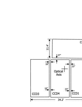
Figure 1: Schematic layout of the Wide Field Camera. All the measures are approximated.

Figure 2: Transmission curves of the U, g’, r’, i’ and Z WFC filters (dotted line). Dashed line shows the quantum efficiency of the detector, where solid line shows to total throughput of the system.

The WFS surveyed $\sim$200 square degrees in different well known regions of sky with data at other wavelengths. The ELAIS regions N1 and N2 were also included. The survey consists of single 600 s exposures in five bands: U, g’, r’, i’ and Z (see figure 2) to magnitude limits of: 23.4, 24.9, 24.0, 23.2, 21.9 respectively (Vega, 5$\sigma$ for a point-like object), i.e., about 1 magnitude deeper than the Sloan Digital Sky Survey (SDSS; York et al., 2000). A total of 108 pointings were done in N1 and N2, covering a total area of 18 square degrees. Typical seeing is about 1.0-1.2^′′. The data are processed by the Cambridge Astronomical Survey Unit (CASU) as described in Irwin & Lewis (2000) and we provide here a short description of the reduction steps. The data are first debiassed (full 2D bias removal is necessary). Bad pixels and columns are then flagged and recorded in confidence maps, which are used during catalogue generation. The CCDs are found to have significant non linearities so a correction using look-up-tables is then applied to all data. Flatfield images in each band are constructed by combining several sky flats obtained in bright sky conditions during the twilight. Exposures obtained in the i’ and Z bands show a significant level of fringing ($\pm$2% and $\pm$6% of sky respectively). In order to remove this effect, master fringe frames are created by combining all the science exposures for each band. These fringe frames are then subtracted from the object exposures. After this removal, the fringing level is reduced to $\pm$0.2% and $\pm$0.4% of sky in the i’ and Z bands respectively. Finally an astrometric solution starts with a rough WCS based on the known telescope and camera geometry and is the progressively refined using the Guide Star Catalogue for a first pass and the APM or PMM catalogues for a final pass. The WFC field distortion is modelled using a zenithal equidistant projection (ZPN; Greisen & Calabretta, 2002). The resulting internal astrometric precision is better than 100 mas over the whole WFC array (based on intercomparison of overlap regions). Global systematics are limited by the precision of the APM and PMM astrometric catalogue systems and are at the level of 300 mas. The object detection is performed in each band separately using a standard APM-style object detection and parametrisation algorithm. Standard aperture fluxes are measured in a set of apertures of radius $r/2$, $r$, $\sqrt{2}\,r$, $2\,r$, $2\,\sqrt{2}\,r$ where $r=3.5$ pixels and an automatic aperture correction (based on the average curve-of-growth for stellar images) is applied to all detected objects.

Photometric calibration is done using series of Landoldt standard stars (Landoldt 1992) with photometry in the SDSS system. For each night a zero point in each filter is derived. For photometric nights the calibration over the whole mosaic has an accuracy of 1-2%. During non-photometric nights, in otherwise acceptable observing conditions, we find that the derived zeropoint systematic errors can be up to 10% or more. Although the pipeline usually successfully flags such nights as non-photometric it still leaves open the problem of what to do about tracking the varying extinction during these nights.

All calibration is by default corrected for the mean atmospheric extinction at La Palma during pipeline processing (0.46 in U, 0.19 in g^′, 0.09 in r^′ and 0.05 in i^′ and Z). Since adjacent camera pointings overlap by several square arcminutes sources in these overlapping regions can be used as magnitude comparison points. However, to use overlapping and hence in general, different CCDs, requires that any repeatable systematics due to, for example, slight differences in the colour equations for each CCD, are first corrected for. Correcting for these is a three stage process. First the twilight flatfields are used to gain-correct each CCD onto a common system. However, since the twilight sky is significantly bluer than most astronomical objects, a secondary correction is made using the measured dark sky levels in each CCD for each filter to provide a correction more appropriate for the majority astronomical object. These corrections, unsurprisingly, are negligible for passbands on the flat part of the generic CCD response curves such as g’ and r’, and amount to 1-2% for the i’ and z’ passbands. The measured dark sky values for the U-band were also consistent with zero correction though with less accuracy due to the low sky levels in the U-band images. Finally any residual offsets between the CCDs are checked for each survey filter using the mean offset between adjacent pointings on photometric survey nights. The only filters requiring significant adjustments to the individual CCD zero points at this stage are CCD3 for U (-3%) and CCD1 for z’ (+3%).

Data from non-photometric nights can now be calibrated in one of two ways: the overlap regions between pointings can be used to directly tie in all the frames onto a common system, with extra weighting given to data taken from photometric nights; the stellar locus in various 2-colour diagrams (in regions of low unchanging extinction like these) can be used to compare colours from all the passbands by cross-correlating the loci between any of the pointings. The colour-colour loci cross-correlations (actually made from a smoothed Hess-like version of the diagrams) give results accurate to better than +/-3% and can be used in conjunction with the overlap results to give overall photometry for the survey to the level of $\approx$2%. The final products include astrometrically calibrated images as well as morphologically classified merged multicolour catalogues, publically available from the WFS web page (http://www.ast.cam.ac.uk/~wfcsur/index.php).

For the purpose of this work, we have also carried out the object detection in the r’ band images using SExtractor (Bertin & Arnouts, 1996). As well as providing a independent check for the extraction method used above, it gives us an extense set of parameters. Aperture magnitudes from SExtractor are found to be in agreement with the ones obtained from the WFS pipeline. Therefore, together with the WFS aperture magnitudes we use MAG_BEST as a measurement of the total magnitude in the r’-band. The galaxy-star classification given by CLASS_STAR is also used to select point-like objects (defined to be CLASS_STAR $>$ 0.8).

As an additional test of our photometric calibration we have correlated the WFS catalogues with those from the Sloan Digital Sky Survey First Data Release (Abazajian et al., 2003). Figure 3 shows the result of this correlation for the r’ band magnitude. Once accounted for the small correction between both filters ($\Delta m=0.09$) the agreement is within 0.04 magnitudes (note also that a second order correction due to different object spectral energy distributions is not removed, so the accuracy is better than the quoted 0.04).

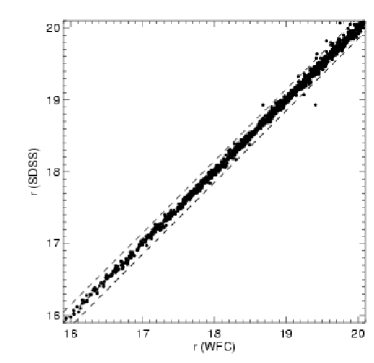
Figure 3: Comparison between WFS and SDSS r’ band magnitudes for point-like objects. A correction $\Delta m=0.09$ has been applied to account for the slight filter and system differences.

3 The mid-IR and radio catalogues

The final analysis of the 15$\mu$m data using the Lari method (Lari et al., 2001) for the ELAIS northern fields has recently been completed (Maccari et al. 2004, in prep). The two main northern fields N1 and N2 are centred at $16^{h}10^{m}01^{s}$ $+54^{\circ}30^{\prime}36^{\prime\prime}$ and $16^{h}36^{m}58^{s}$ $+41^{\circ}15^{\prime}43^{\prime\prime}$ respectively. We have obtained a sample of 1056 sources (490 in N1 and 566 in N2) to a $5\sigma$ flux limit of 0.45 mJy. This catalogue includes sources detected in deeper observations (in particular, the central 40^′ $\times$40^′ N2 area has been observed three times) so this flux limit is not homogenous over the whole survey area.

As part of the multiwavelenth follow-up observations carried out in these regions Ciliegi et al. (1999) have conducted a survey at 20 cm using the VLA in its C configuration, covering 4.22 sq. deg. in the N1, N2 and N3 areas. They detect a total of 867 sources (362 in N1, 329 in N2 and 176 in N3) above a flux limit 0.135 mJy in the deeper observations or 1.15 mJy over the shallower ones. We have selected sources for which we have optical data from the WFS (i.e., sources in N1 and N2). Multi-component sources (flagged in the catalogue as ’A’, ’B’ or ’C’ components) have been removed and only the calculated central position considered (’T’ in the catalogue).

4 Optical identifications of ELAIS sources

As shown in Lari et al. (2001), the positional errors in RA and DEC for the ELAIS sources result from the combination of three quantities: the finite spatial sampling ($\sigma_{\rm s}$), the reduction method ($\sigma_{\rm r}$) and the pointing accuracy ($\sigma_{\rm P}$). The simulation work carried out in the ELAIS fields yield next relations:

$$\sigma_{\rm s+r}({\rm RA})=1.00+17.17\times{\rm e}^{(-0.57\times{\rm S/N})}$$ (1)

$$\sigma_{\rm s+r}({\rm DEC})=1.06+1.21\times{\rm e}^{(-0.16\times{\rm S/N})}$$ (2)

These equations have been used to estimate the positional errors due to mapping and reduction method as a function of each source’s signal-to-noise ratio, S/N.

The errors introduced by uncertainties in the ISOCAM pointing have been estimated by correlating the ISO sources with the USNO catalogue of optical objects (Monet, 1998). For each raster, both catalogues have been correlated using a maximum search distance of 12^′′. The median of the offsets values for all the ISO-USNO associations have been calculated,$\sigma_{\rm P}({\rm RA})$, $\sigma_{\rm P}({\rm DEC})$. Each source position has then been corrected for the offset found for each raster. The final positional error is then:

$$\sigma_{\rm RA}^{2}=\sigma_{\rm s+r}^{2}({\rm RA})+\sigma_{\rm P}^{2}({\rm RA})+0.4^{2}$$ (3)

$$\sigma_{\rm DEC}^{2}=\sigma_{\rm s+r}^{2}({\rm DEC})+\sigma_{\rm P}^{2}({\rm DEC})+0.4^{2}$$ (4)

where a $\sigma=0.4$^′′ has been added to account for the optical errors. Typical positional errors are $\sigma\sim 3$^′′.

Figure 4: Offsets between 15$\mu$m and optical positions (left) and between radio and optical positions (right).

The correlation between ELAIS 15$\mu$m sources and optical objects has been carried out using a likelihood ratio method (Sutherland & Saunders, 1992), similar to the one which has been successfully applied to the identification of 15$\mu$m sources detected by ISO in the HDF-N by Mann et al. (1997).

The probability that an optical object of magnitude $m$ is the true counterpart of a source with an error ellipse defined by its major axis, $\sigma_{1}$, and minor axis, $\sigma_{2}$, separated a distance $r$ is given by

$$\mathcal{L}=\frac{Q(m)exp(-r^{2}/2)}{2\pi\sigma_{1}\sigma_{2}N(m)}$$ (5)

where $Q$ and $N$ are the magnitude distributions of the sources and objects respectively. The reliability of such identification is

$$\mathcal{R}_{j}=\frac{\mathcal{L}_{j}}{\sum_{i}\mathcal{L}_{i}+(1-Q)}$$ (6)

The identification process is carried out as follows. For each ELAIS 15$\mu$m source, all optical objects within a distance of 20^′′ are selected. This list is our candidate list. For each object in our candidate list we calculate the values of the likelihood and reliability as given by equations above. The likelihood value (equation 5) gives us the probability that a candidate is the true optical counterpart of the source; but it only provides information about the probability of each candidate being the correct counterpart. The reliability (equation 6) provides information about the number of candidates with high likelihood values. A candidate will have large values of likelihood and reliability if it is the only probable counterpart of a source. In case where there are multiple probable counterparts (in the sense of high likelihood), they all will have low values of reliability.

A candidate is selected to be the correct optical identification of a ELAIS source when $\mathcal{L}>0.8$. Sources for which no candidates meet this requirement are flagged as blank fields and represent $\sim 8\%$ of the total sample (section 7). Sources for which there are more than one candidate meeting this requirement, and have low values of reliability, are flagged as having multiple possible counterpart and represent $\sim 8\%$ of the sample. Finally bright stars, saturated in the WFS CCD data are also flagged; note that their astrometric accuracy is poor. They represent $\sim 22\%$ of the sample. Figure 4 (left) shows the offsets between ISO and optical identifications, excluding saturated stars. Uncertainties are well fitted by a Gaussian distribution of $\sigma\sim 1$^′′.

Optical identification of the ELAIS radio sources detected in the N1 and N2 areas is carried out using a similar procedure. In this case the radio catalogue provides measurements of the positional errors, so these are used in our likelihood ratio algorithm. An optical counterpart is found for 389 out of the 691 sources, i.e., there is a 44% of blank fields. Figure 4 (right) shows the offsets between radio sources and the optical counterpart. This provides a confirmation of the good accuracy of the astrometry of the 15 $\mu$m sources.

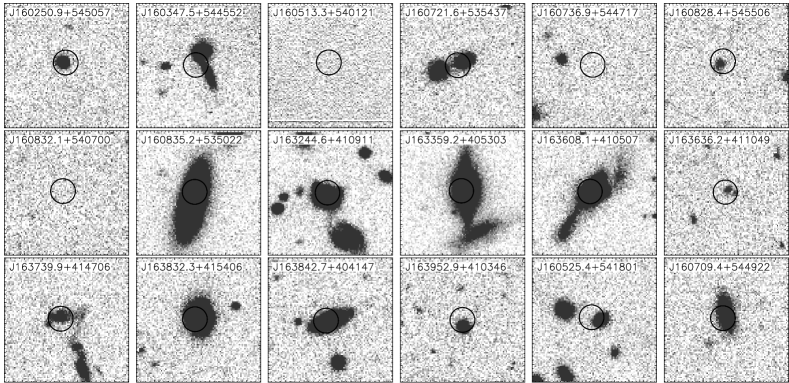
Figure 5: Example r’-band postage stamps of 15$\mu$m detected sources. Each chart is 30^′′ $\times$30^′′ in size.

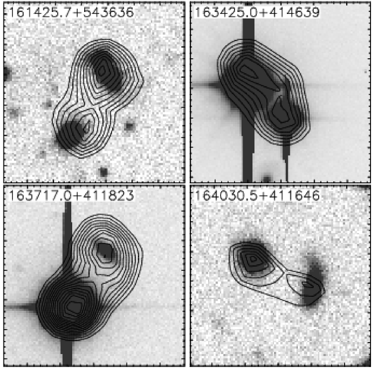
Figure 6: Double sources merged in the ELAIS 15$\mu$m catalogue. Mid-IR contours starting at $5\sigma$ and increasing at steps of $1\sigma$ are shown plotted over the r’-band image. Each chart is 30^′′ $\times$30^′′ in size.

Figure 5 shows some example finding charts of sources detected at 15$\mu$m. These charts are 30^′′ $\times$30^′′ in size and have been extracted from the r’-band images. Also shown a 3^′′ radius circle centered on the ISO position. As shown in section 5 a large fraction of the sources are associated with bright galaxies. Example of sources with more than one plausible counterpart is given by e.g., J163636.2+411049. The most likely counterpart is an object with r’=21.8 at a distance of 1.1 arcsec from the ISO position. Its likelihood is 0.988 and reliability is 0.773. There is another source of r’=23.0 separated 2 arcsec from the ISO position with likelihood 0.960 and reliability 0.227. We choose the first one as the optical counterpart (based on higher values of likelihood and reliability) of the ISO source and flag it has having more than one plausible counterpart. Examples of these are also J160347.5+544552 and J160721.6+535437.

There are four ELAIS sources which have been merged in the final analysis 15 $\mu$m catalogue (figure 6). Both possible counterparts are given in the optical identification catalogue and the 15 $\mu$m flux is assigned to both.

The table of optical identifications is available electronically in: http://www.ast.cam.ac.uk/~eglez/eid. Also included are postage stamps for all the sources in the r’ band (grayscale and contours) as well as multiband grayscale finding charts.

The format of the table is as follows:

Column 1.

International Astronomical Unit name of the source. Sources are listed in RA order. Sources detected in N2 are listed after those detected in N1.

Column 2.

ISO coordinates (J2000) of the sources.

Column 3.

Coordinates (J2000) of the optical counterpart of the source.

Columns 4 to 8.

Aperture magnitude in U, g’, r’, i’ and Z bands (aperture of radius 3.5 pixels – 1.16^′′).

Column 9.

Total r’-band magnitude as provided by SExtractor MAG_BEST parameter.

Columns 10 to 15.

Errors in previous magnitudes.

Columns 16 to 21.

Stellar classification as provided by WFS and SExtractor CLASS_STAR parameters.

Columns 22, 23 and 24.

Distance, $\Delta\alpha$ and $\Delta\delta$ between the ELAIS source and the optical association.

Columns 25 and 26.

Likelihood of the identification formated as $\mathcal{L}/(1+\mathcal{L})$ and reliability.

Columns 27 and 28.

Flux at 15$\mu$m and signal-to-noise ratio.

Column 29.

Optical flag code as follows. B1: source in a gap between chips or in the edge of a chip, B3: most likely optical identification when multiple counterparts, B4: blank field, B7: bright saturated star, B9: other plausible optical identification when multiple counterparts.

5 Magnitude distributions

Figure 7 shows the magnitude distribution of the optical counterparts of ELAIS 15 $\mu$m sources. The first peak at r’$\sim$12-13 is caused by bright stars which are saturated in the WFS data. The second peak, due to extra-galactic objects, is located at r’$=18$. Most of the extragalactic sources are then associated with optically bright objects. A tail of faint objects is present at r’$>$20.

In order to calculate the percentage of chance associations, especially at the faintest magnitudes, we have simulated four catalogues in each N1 and N2 regions by offsetting 20 arcsec in R.A. and DEC from the ISO position in four directions. The likelihood ratio technique was used to associate the sources in these new catalogues in the same way as done for the real ones. The identifications obtained provides the distribution of chance associations. This percentage is $\sim$5% for r’$\leq$20 and increases to 20% at r’=24.

Figure 7 also shows the magnitude distribution of point like objects. About 16% of the objects with magnitude r’$>$15 are classified as point like. Their magnitude distribution has a peak at r’$\sim$19, a magnitude fainter than that for galaxies.

Figure 7: Magnitude distribution of 15 $\mu$m sources in ELAIS N1 and N2. Hatched histogram shows the distribution of point-like sources. Last bin, with right arrow symbols, represent the objects without optical counterpart.

Figure 8: Magnitude distribution of 1.4 GHz radio sources in ELAIS N1 and N2. Hatched histogram shows the distribution of point-like sources. Last bin, with right arrow symbols, represent the objects without optical counterpart.

The magnitude distribution of radio sources is shown in figure 8. Unlike the distribution of mid-IR sources the number of sources show an increase at fainter magnitudes. The number of point-like objects is very low (hatched histogram) but the reliability of the CLASS_STAR parameter in SExtractor decreases at faint magnitudes and fails at r’$\geq$23.

6 Optical to infrared fluxes

Figure 9 shows the mid-IR to optical fluxes for the ELAIS sources. Stars have typically low mid-IR fluxes compared to their optical fluxes and are located in the region where their mid-IR flux is ten times smaller than their optical flux. Most of the extragalactic objects have mid-IR fluxes between 1 and 100 times their optical fluxes. According to models of infrared galaxies previously published Rowan-Robinson (2001), galaxies whose infrared emission is dominated by cirrus are located in the region $0<\log S_{15}/S_{r^{\prime}}<1$. More infrared “active” galaxies, i.e., starbursts, AGN and Arp220-like objects are located in regions of mid-IR flux 10 times to 100 times larger than their optical flux.

Optical colours can be used to discriminate between AGNs and galaxies. As figure 10 shows AGNs are typically 0.5 magnitudes bluer than galaxies (and as shown in  10, about 1 magnitude fainter). There is a population of point-like objects with galaxy-like colours, presumable highly obscured. Their overall spectra can be well fitted by a galaxy SED (Rowan-Robinson et al., 2003).

The radio to optical flux ratio versus magnitude and versus optical colour are shown in figures 11 and 12 for the 1.4 GHz sources with optical counterpart. Those sources which show emission at 15$\mu$m are also marked with black symbols. Most of the 15 $\mu$m- radio coincidences are objects with magnitudes 15$<$r’$<$20 for which the cirrus component is the most plausible source of the infrared and radio emission.

Attending to their radio, mid-IR and optical properties (see figure 13) the bulk of the 15 $\mu$m sources (those with $0<\log S_{15}/S_{r^{\prime}}<2$) can be explained as a mixture of cirrus-dominated galaxies and starburst with smaller fractions of Arp220-like objects and AGN.

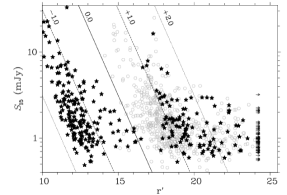
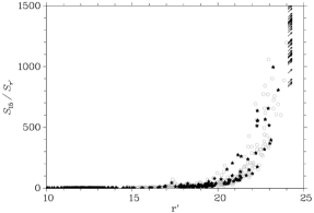
Figure 9: Optical to infrared flux ratio for 15$\mu$m sources with optical counterpart. Top figure shows the mid-IR flux versus optical magnitude. Point-like classified object are shown as black stars while galaxies are shown as gray circles. Lines of constant flux ratio $\log(S_{15}/S_{r^{\prime}})=-1.0,0.0,+1.0,+2.0$ are also shown. Blank fields are displayed using a right arrow. Bottom figure shows $\log(S_{15}/S_{r^{\prime}})$ versus optical magnitude.

6.1 Population with large infrared-to-optical flux ratio

Figure  9 also shows the existence of a population of objects with extreme mid-IR to optical fluxes and faint optical magnitudes. The nature of this population can only be studied with detailed spectroscopic followup observations. Two of the point like objects in this region of the diagram have spectroscopic redshifts. The object associated with ELAISC15_J164021.5+413925 has a 15$\mu$m flux of $S_{15}=2.98$ mJy, an optical magnitude of r’$=20.3$ and a redshift $z=0.60$ (Perez-Fournon et al. 2003, in prep.). Its luminosity is $L=10^{11}\,L_{\odot}$. The second object is associated with ELAISC15_J163655.8+405909. It has a 15$\mu$m flux of $S_{15}=0.72$ mJy, an optical magnitude of r’$=23.9$ and a redshift $z=2.61$ (Willott et al., 2003). Its luminosity is $L=10^{12}\,L_{\odot}$ ($H_{0}=65,\Omega_{m}=0.3,\Lambda_{0}=0.7$).

Using infrared models of starburst galaxies and AGN, and adding reddening (as modeled by Calzetti et al. (2000)), we can explain the nature of this population. Objects with $\log S_{15}/S_{r^{\prime}}>2$ can be explained as luminous starburst galaxies, with luminosities $L\sim 10^{12}\,L_{\odot}$, at redshifts $z\sim 0.7$ and reddening $A_{v}\sim 1-1.5$. Fainter optical objects with $\log S_{15}/S_{r^{\prime}}\sim 3$ have typically larger luminosities $L>10^{13}\,L_{\odot}$, redshifts $z\sim 1.3$ and reddening $A_{v}\sim 2$. Luminous AGN, with $L\sim 10^{12}\,L_{\odot}$, also populate this area.

The association of this sources with very reddened objects supports the assumption that the objects with $S_{15}/S_{r^{\prime}}>100$ in figure 9 may represent a new population of heavily obscured starbursts and type 2 AGN.

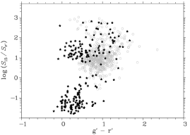
Figure 10: Infrared to optical flux ratio versus optical colour $g^{\prime}-r^{\prime}$. Symbols as in figure 9.

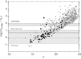
Figure 11: Radio to optical flux ratio versus optical magnitude. Black symbols represent the sources detected also at 15$\mu$m (dots: galaxies, stars: point-like objects). Hatched areas represent the range predicted by different infrared galaxy types in the range $0<z<1.5$ (redshift increases from bottom to top in each area; dashed line shows the location of $z=1.0$).

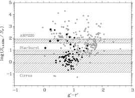
Figure 12: Radio to optical flux ratio versus optical colour. Symbols as in figure 11.

Figure 13: Radio to mid-IR flux ratio versus mid-IR to optical flux ratio. Symbols as in figure 11. Lines show the location of different infrared galaxy models..

7 Blank fields

A percentage of 8% of the 15$\mu$m sources (38 in N1, 67 in N2) do not have an optical counterpart down to the optical limits of data described in previous sections. All of them have infrared fluxes $S_{15}<3$ mJy, and only 3 show a plausible association with a radio source (table 1). Blank fields are probably the extreme version of the objects found at $\log S_{15}/S_{r^{\prime}}>2$. Using the same model galaxies as before, we find that starburst galaxies with luminosities $L\sim 10^{13}\,L_{\odot}$, $z\sim 1.$ and $A_{v}\sim 3-4$ may populate this region. The cause of the infrared emission and the starburst activity may be the merger of galaxies ir the formation of a protogalaxy although the accuracy of this hypotheses cannot be tested with these data.

Table 1: ELAIS blank fields with a radio source nearest than 3^′′ from the ISO position. Fluxes are given in mJy.

Name	ISO Coords (J2000)	$S_{15\mu\rm m}$	$S_{20\rm cm}$
J160734.3+544216	16 07 34.40 +54 42 15.6	1.51$\pm$0.19	0.37$\pm$0.02
J163505.4+412508	16 35 05.71 +41 25 11.2	0.83$\pm$0.09	0.38$\pm$0.02
J163511.4+412255	16 35 11.54 +41 22 57.4	0.72$\pm$0.09	0.94$\pm$0.02

8 Summary

The association of sources detected at 15$\mu$m in the ELAIS N1 and N2 areas with optical objects is presented. A 92% of the sample presents an optical identification to r’=24. The magnitude distribution presents a maximum at r’=18 and a tail which extends to fainter magnitudes. The distribution of point-like objects presents a maximum one magnitude fainter. The mid-IR to optical flux ratios, $S_{15}/S_{r^{\prime}}$, of the bright optical sources are in the range 1 to $10^{2}$ and can be explained using simple models of cirrus, starbursts, AGN and Arp220 spectral energy distributions. The tail of faint objects, show larger $S_{15}/S_{r^{\prime}}$, from $10^{2}$ to $10^{3}$ and can only be explained assuming large luminosities and obscurations. Point like objects show bluer g’-r’ colour while higher mid-IR to optical flux ratio than galaxies. The remaining 8% of objects not identified are faint in the mid-IR , with a $15\mu$m flux lower than 3 mJy. However, their mid-IR-to-optical flux ratio is larger than $10^{3}$ favouring the interpretation that they are associated with starbursts or AGNs at high redshifts and highly obscured. The identification of radio sources in the same areas is also presented. Their magnitude distribution shows an increase on the number of sources towards faint magnitudes. The number of unidentified objects is 44%.

9 Acknowledgements

EAGS aknowledges support by EC Marie Curie Fellowship MCFI-2001-01809 and PPARC grant PPA/G/S/2000/00508. The ELAIS consortium also acknowledges support from EC Training Mobility Research Networks ’ISO Survey’ (FMRX-CT96-0068) and ’Probing the Origin of the Extragalactic background light (POE)’ (HPRN-CT-2000-00138) and from PPARC. This paper is based on observations with ISO, an ESA project, with instruments funded by ESA Member States (especially the PI countries: France, Germany, the Netherlands and the United Kingdom) and with participation of ISAS and NASA. The INT is operated on the island of La Palma by the Isaac Newton Group in the Spanish Observatorio del Roque de los Muchachos of the Instituto de Astrofisica de Canarias.

References

- Abazajian et al. (2003) Abazajian M. et al., 2003, astro-ph/0305492
- Bertin & Arnouts (1996) Bertin E., Arnouts S., 1996, A&AS, 117, 393
- Calzetti et al. (2000) Calzetti D., Armus L., Bohlin R. C., Kinney A. L., Koornneef J., Storchi-Bergmann T., 2000, ApJ, 533, 682
- Cesarsky et al. (1996) Cesarsky C. J. et al., 1996, A&A, 315, L32
- Ciliegi et al. (1999) Ciliegi P. et al., 1999, MNRAS, 302, 222
- Greisen & Calabretta (2002) Greisen E. W., Calabretta M. R., 2002, A&A, 395, 1061
- Kessler et al. (1996) Kessler M. F. et al., 1996, A&A, 315, L27
- Lari et al. (2001) Lari C. et al., 2001, MNRAS, 325, 1173
- Lemke et al. (1996) Lemke D. et al., 1996, A&A, 315, L64
- Lonsdale et al. (2003) Lonsdale C. J. et al., 2003, PASP, 115, 897
- Mann et al. (1997) Mann R. G. et al., 1997, MNRAS, 289, 482
- McMahon et al. (2001) McMahon R. G., Walton N. A., Irwin M. J., Lewis J. R., Bunclark P. S., Jones D. H., 2001, New Astronomy Review, 45, 97
- Monet (1998) Monet D. G., 1998, Bulletin of the American Astronomical Society, 30, 1427
- Oliver et al. (2000) Oliver S. et al., 2000, MNRAS, 316, 749
- Rowan-Robinson et al. (2003) Rowan-Robinson M. et al., 2003, astro-ph/0308283
- Rowan-Robinson (2001) Rowan-Robinson M., 2001, New Astronomy Review, 45, 631
- Sutherland & Saunders (1992) Sutherland W., Saunders W., 1992, MNRAS, 259, 413
- Willott et al. (2003) Willott C. J. et al., 2003, MNRAS, 339, 397
- York et al. (2000) York D. G. et al., 2000, AJ, 120, 1579