The origin and implications of
dark matter anisotropic cosmic infall on $\approx L_{\star}$ haloes

Abstract

We measure the anisotropy of dark matter flows on small scales ($\leq 500$ kpc) in the near environment of haloes using a large set of simulations. We rely on two different approaches to quantify the anisotropy of the cosmic infall: we measure the flows at the haloes’ virial radius while describing the infalling matter via fluxes through a spherical shell; we measure the spatial and kinematical distributions of satellites and substructures around haloes detected by the subclump finder ADAPTAHOP first described in the appendix B. The two methods are found to be in agreement both qualitatively and quantitatively via one and two points statistics.
The peripheral and advected momentum is correlated with the spin of the embeded halo at a level of $30\%$ and $50\%$. The infall takes place preferentially in the plane perpendicular to the direction defined by the halo’s spin. We computed the excess of equatorial accretion both through rings and via a harmonic expansion of the infall.
The level of anisotropy of infalling matter is found to be $\sim 15\%$. The substructures have their spin orthogonal to their velocity vector in the halo’s rest frame at a level of about $5\%$, suggestive of an image of a flow along filamentary structures which provides an explanation for the measured anisotropy. Using a ‘synthetic’ stacked halo, it is shown that the satellites’ positions and orientations relative to the direction of the halo’s spin are not random even in projection. The average ellipticity of stacked haloes is $10\%$, while the alignment excess in projection reaches $2\%$. All measured correlations are fitted by a simple 3 parameters model.
We conclude that a halo does not see its environment as an isotropic perturbation, investigate how the anisotropy is propagated inwards using perturbation theory, and discuss briefly implications for weak lensing, warps and the thickness of galactic disks.

1 Introduction

Isotropy is one of the fundamental assumptions in modern cosmology and is widely verified on very large scales, both in large galaxies’ surveys and in numerical simulations. However on scales of a few Mpc, the matter distribution is structured in clusters and filaments. The issue of the anisotropy down to galactic and cluster scales has long been studied, as it is related to the search for large scale structuration in the near-environment of galaxies. For example, both observational study (e.g. West (1994), Plionis & Basilakos (2002), Kitzbichler & Saurer (2003)) and numerical investigations (e.g. Faltenbacher et al. (2002)) showed that galaxies tend to be aligned with their neighbours and support the vision of anisotropic mergers along filamentary structures. On smaller scales, simulations of rich clusters showed that the shape and velocity ellipsoids of haloes tend to be aligned with the distribution of infalling satellites which is strongly anisotropic (Tormen (1997)). However the point is still moot and recent publications did not confirm such an anisotropy using resimulated haloes; they proposed 20$\%$ as a maximum for the anisotropy level of the satellites distribution (Vitvitska et al. (2002)).

When considering preferential directions within the large scale cosmic web, the picture that comes naturally to mind is one involving these long filamentary structures linking large clusters to one other. The flow of haloes within these filaments can be responsible for the emergence of preferential directions and alignments. Previous publications showed that the distributions of spin vectors are not random. For example, haloes in simulations tend to have their spin pointing orthogonally to the filaments’ direction (Faltenbacher et al. (2002)). Furthermore, down to galactic scales, the angular momentum remains mainly aligned within haloes (Bullock et al. (2001)). Combined with the results suggesting that haloes’ spins are mostly sensitive to recent infall (van Haarlem & van de Weygaert (1993)), these alignment properties fit well with accretion scenarii along special directions : angular momentum can be considered as a good marker to test this picture.

Most of these previous studies focused on the fact that alignments and preferential directions are consequences of the formation process of haloes. However, the effects of such preferential directions on the inner properties of galaxies have been less addressed. It is widely accepted that the properties of galaxies partly result from their interactions with their environments. While the amplitude of the interactions is an important parameter, some issues cannot be studied without taking into account the spatial extension of these interactions. For example, a warp may be generated by the torque imposed by infalling matter on the disk (Ostriker & Binney (1989), López-Corredoira et al. (2002)) : the direction but also the amplitude of the warp are a direct consequence of the spatial configuration of the perturbation. Similarly, it is likely that disks’ thickening due to infall is not independent of the incoming direction of satellites (e.g. Quinn et al. (1993), Velazquez & White (1999), Huang & Carlberg (1997)).

Is it possible to observe the small-scale alignment ? In particular, weak lensing deals with effects as small as the level of detected anisotropy (if not smaller) (e.g. Hatton & Ninin (2001), Croft & Metzler (2000), Heavens et al. (2000)), hence the importance to put quantitative constraints on the existence of alignments on small scales. Therefore, the present paper also addresses the issue of detecting preferential projected orientations on the sky of substructures within haloes.

Our main aim is to provide quantitative measurements to study the consequences of the existence of preferential directions on the dynamical properties of haloes and galaxies, and on the observation of galaxy alignments. Hence our point of view is more galactocentric (or cluster-centric) than previous studies. We search for local alignment properties on scales of a few hundred kpc. Using a large sample of low resolution numerical simulations, we aim to extract quantitative results from a large number of halo environments. We reach a higher level of statistical significance while reducing the cosmic variance. We applied two complementary approaches to study the anisotropy around haloes: the first one is particulate and uses a new substructure detection tool ADAPTAHOP, the other one is the spherical galactocentric fluid approach. Using two methods, we can assess the self-consistency of our results.

After a brief description of our set of simulations ($\S 2$), we describe the galactocentric point of view and study the properties of angular momentum and infall anisotropy measured at the virial radius ($\S 3$). In ($\S 4$) we focus on anisotropy in the distribution of discrete satellites and substructures and we study the properties of the satellites’ proper spin , which provides an explanation for the detected anisotropy. In ($\S 5$) we discuss the level of anisotropy as seen in projection on the plane of the sky. We then investigate how the anisotropic infall is propagated inwards and discuss the possible implications of our results to weak lensing and to the dynamics of the disk through warp generation and disk thickening ($\S 6$). Conclusions and prospects follow. The appendix describes the substructures detection tool ADAPTAHOP together with the relevant aspects of one point centered statistics on the sphere. We also formally derive there the perturbative inward propagation of infalling fluxes into a collisionless self gravitating sphere.

2 Simulations

In order to achieve a sufficient sample and ensure a convergence of the measurements, we produced a set of $\sim 500$ simulations. Each of them consists of a 50 $h^{-1}$ Mpc³ box containing $128^{3}$ particles. The mass resolution is $5\cdot 10^{9}M\odot$. A $\Lambda$CDM cosmogony ($\Omega_{m}=0.3$, $\Omega_{\Lambda}=0.7$, $h=0.7$ and $\sigma_{8}=0.928$) is implemented with different initial conditions. These initial conditions were produced with GRAFIC (Bertschinger (2001)) where we chose a BBKS (Bardeen et al. (1986)) transfer function to compute the initial power spectrum. The initial conditions were used as inputs to the parallel version of the treecode GADGET (Springel et al. (2001)). We set the softening length to 19 $h^{-1}$ kpc. The halo detection was performed using the halo finder HOP (Eisenstein & Hut (1998)). We employed the density thresholds suggested by the authors ($\Delta_{\mathrm{outer}}=80,\delta_{\mathrm{saddle}}=2.5\delta_{\mathrm{outer}},\delta_{\mathrm{peak}}=3.\delta_{\mathrm{outer}}$) As a check, we computed the halo mass distribution. It is shown in Fig. 1 and compared to the Press-Schechter mass function (Press & Schechter (1974)). The measured distribution is in agreement with the theoretical curve up to masses $\sim 3\cdot 10^{14}M_{\odot}$ (100 000 particles), which validates our completeness in mass.

Figure 1: The number density, $dN/dM$, of haloes with a mass M (within dM) detected in our simulations at redshift zero (solid line) compared to the distribution expected by Press-Schechter (dashed line). The agreement is good for masses between $3\cdot 10^{11}M_{\odot}$ and $3\cdot 10^{14}M_{\odot}$.

As an other means to check our simulations and to evaluate the convergence ensured by our large set of haloes, we computed the probability distribution of the spin parameter $\lambda^{\prime}$, defined as (Bullock et al. (2001)):

$$\lambda^{\prime}\equiv\frac{J}{\sqrt{2}MVR_{200}}.$$ (1)

Here $J$ is the angular momentum contained in a sphere of virial radius $R_{200}$ with a mass M and $V^{2}=GM/R_{200}$. The measurement was performed on 100 000 haloes with a mass larger than $5\cdot 10^{12}M_{\odot}$ as explained in the next section. The resulting distribution for $\lambda^{\prime}$ is shown in Fig. 2. The distribution $P(\lambda^{\prime})$ is well fitted by a log-normal distribution (e.g. Bullock et al. (2001)):

$$P(\lambda^{\prime}){{\mathrm{d}}}\lambda^{\prime}=\frac{1}{\lambda^{\prime}\sqrt{2\pi}\sigma}\exp\left(-\frac{\ln^{2}(\lambda^{\prime}/\lambda_{0}^{\prime})}{2\sigma^{2}}\right){{\mathrm{d}}}\lambda^{\prime}.$$ (2)

We found $\lambda_{0}^{\prime}=0.0347\pm 0.0006$ and $\sigma=0.63\pm 0.02$ as best-fit values and they are consistent with parameters found by Peirani et al. (2003) ($\lambda^{\prime}=0.035$ and $\sigma=0.57$) but our value of $\sigma$ is slightly larger. However, using $\sigma=0.57$ does not lead to a significantly different result. The value of $\sigma$ is not strongly constrained and no real disagreement exists between our and their best-fit values. The halo’s spin, on which some of the following investigations are based, is computed accurately.

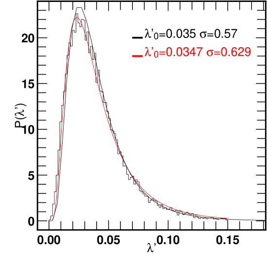
Figure 2: The distribution of the spin parameter $\lambda^{\prime}$ defined as $\lambda^{\prime}\equiv J/(\sqrt{2}MVR_{200})$ computed using 100 000 haloes with a mass greater than $5\cdot 10^{12}M_{\odot}$. The distribution can be fit with a log-normal function with parameters $\lambda_{0}^{\prime}=0.0347\pm 0.0006$ and $\sigma=0.63\pm 0.02$ (red line). The curve parametrized by $\lambda_{0}^{\prime}=0.035$ and $\sigma=0.57$ is also shown (black line). The two results are almost concurrent, indicating that the value of $\sigma$ is not so strongly constrained using a log-normal distribution.

3 A galactocentric point of view

The analysis of exchange processes between the haloes and the intergalactic medium will be carried out using two methods. The first one can be described as ‘discrete’. The accreted objects are explicitly counted as particles or particle groups. This approach will be applied and discussed later in this paper. The other method relies on measuring directly relevant quantities on a surface at the interface between the halo and the intergalactic medium. In this approach, the measured quantities are scalar, vector or tensor fluxes, and we assign to them flux densities. The flux density representation allows us to describe the angular distribution and temporal coherence of infalling objects or quantities related to this infall. The formal relation between a flux density, ${\mbox{\boldmath$\varpi$}}({\bf\Omega})$, and its associated total flux through a region $S$, $\Phi$, is:

$$\Phi\equiv\int_{S}{\mbox{\boldmath$\varpi$}}({\bf\Omega})\cdot{{\mathrm{d}}}{\bf\Omega},$$ (3)

where ${\bf\Omega}$ denotes the position on the surface where $\varpi$ is evaluated and ${{\mathrm{d}}}{\bf\Omega}$ is the surface element normal to this surface. Examples of flux densities are mass flux density, $\rho{\bf v_{r}}$, or accreted angular momentum, $\rho{\bf v_{r}}{\bf L}$. In particular, this description in terms of a spherical boundary condition is well-suited to study the dynamical stability and response of galactic systems. In this section, these fields are used as probes of the environment of haloes.

3.1 Halo analysis

Once a halo is detected, we study its environment using a galactocentric point of view. The relevant fields ${{\mbox{\boldmath$\varpi$}}}({\bf{\mbox{\boldmath$\Omega$}}})$ are measured on the surface of a sphere centered on the halo’s centre of mass with a $R_{200}$ radius (where $3M/(4\pi R_{200}^{3})\equiv 200\overline{\rho}$) (cf. fig .3). There is no exact, nor unique, definition of the halo’s outer boundary and our choice of a $R_{200}$ (also called the virial radius) is the result of a compromise between a large distance to the halo’s center and a good signal-to-noise ratio in the spherical density fields determination.

We used $40\times 40$ regularly sampled maps in spherical angles ${\bf\Omega}=(\vartheta,\phi)$, allowing for an angular resolution of 9 degrees. We take into account haloes with a minimum number of $1000$ particles, which gives a good representation of high density regions on the sphere. This minimum corresponds to $5\cdot 10^{12}M_{\odot}$ for a halo, and allows us to reach a total number of 10 000 haloes at z=2 and 50 000 haloes at z=0. This range of mass corresponds to a somewhat high value for a typical $L_{*}$ galaxy but results from our compromise between resolution and sample size. Detailed analysis of the effects of resolution is postponed to Aubert & Pichon (2004).

The density, $\rho({\bf{\mbox{\boldmath$\Omega$}}}$), on the sphere is computed using the particles located in a shell with a radius of $R_{200}$ and a thickness of $R_{200}/10$ (this is quite similar in spirit to the count in cell techniques widely used in analyzing the large scale structures, but in the context of a sphere the cells are shell segments). Weighting the density with quantities such as the radial velocity or the angular momentum of each particle contained within the shell, the associated spherical fields, $\rho{\bf v_{r}}({{\mbox{\boldmath$\Omega$}}})$ or $\rho{\bf L}({{\mbox{\boldmath$\Omega$}}})$, can be calculated for each halo. Two examples of spherical maps are given in Fig. 3. They illustrate a frequently observed discrepancy between the two types of spherical fields, $\rho({\bf{\mbox{\boldmath$\Omega$}}}$) and $\rho{\bf v_{r}}({{\mbox{\boldmath$\Omega$}}}$). The spherical density field, $\rho({\bf{\mbox{\boldmath$\Omega$}}}$), is strongly quadrupolar, which is due to the intersection of the halo triaxial 3-dimensional density field by our 2-dimensional virtual sphere. By contrast the flux density of matter, $\rho{\bf v_{r}}({{\mbox{\boldmath$\Omega$}}}$), does not have such quadrupolar distribution. The contribution of halo particles to the net flux density is small compared to the contribution of particles coming from the outer intergalactic region.

Figure 3: A galactocentric point of view of the density field, $\rho({\bf{\mbox{\boldmath$\Omega$}}})$ (top) and of the flux density of mass, $\rho{\bf v_{r}}({\bf{\mbox{\boldmath$\Omega$}}})$, surrounding the same halo (bottom). This measurement was extracted from a $\Lambda$CDM cosmological simulation. The considered halo contained about $10^{13}M_{\odot}$ or 2000 particles. The high density zones are darker. The density’s spherical field shows a strong quadrupolar component with high density zones near the two poles while this component is less important for the mass flux density field measured on the sphere. This discrepancy between the two spherical fields is common and reflects the shape of the halo as discussed in the main text.

3.2 Two-points statistics: advected momentum and halo’s spin

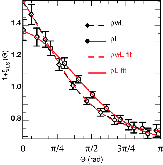
Figure 4: Excess probability, $1+\xi_{\mathrm{LS}}(\theta)$, of the angle, $\theta$, between the halo’s spin ($\bf S$) and the angular momentum (${\bf L}_{T}$ for total, or ${\bf L}_{A}$ for accreted) measured on the virial sphere using the fluid located at the virial radius. Here ${\bf L}_{T}$ represents the total angular momentum measured on the virial sphere (corresponding curve : solid line, circle symbols) and ${\bf L}_{A}$ the total accreted angular momentum measured on the sphere (corresponding curve: dashed line, diamond symbols). The error bars represent the $3\sigma$ dispersion measured on subsamples of 10 000 haloes. The correlation takes into account the uncertainty on the angle determination due to the small number of particles at the virial radius. Here $\xi_{\mathrm{LS}}(\theta)\equiv 0$ would be expected for an isotropic distribution of angles between $\bf S$ and $\bf L$ while the measured distributions indicate that the aligned configuration ($\theta\sim 0$) is significantly more likely. The two excess probability distibutions are well-fitted by Gaussian functions (red curves: see main text).

The influence of infalling matter on the dynamical state of a galaxy depends on whether or not the infall occurs inside or outside the galactic plane. If the infalling matter is orbiting in the galactic plane, its angular momentum is aligned with the angular momentum of the disk. Taking the halo’s spin as a reference for the direction of the ‘galactic’ plane, we want to quantify the level of alignment of the orbital angular momentum of peripheral structures (i.e. as measured on the virial sphere) relative to that spin. The inner spin $\bf{S}$ is calculated using the positions-velocities $({\bf r_{\mathrm{part}}},{\bf v_{\mathrm{part}}})$ of the particles inside the $R_{200}$ sphere in the centre of mass rest frame $({\bf r_{\mathrm{0}}},{\bf v_{\mathrm{0}}})$:

$${\bf S}=\sum_{\mathrm{part}}({\bf r_{\mathrm{part}}-r_{\mathrm{0}}})\times({\bf v_{\mathrm{part}}-v_{\mathrm{0}}}).$$ (4)

${\bf r_{\mathrm{0}}}$ is the position of the halo centre of mass, while ${\bf v_{\mathrm{0}}}$ stands for the average velocity of the halo’s particles. This choice of rest frame is not unique; another option would have been to take the most bounded particle as a reference. Nevertheless, given the considered mass range, no significant alteration of the results is to be expected. The total angular momentum, ${\bf L}_{T}$ (measured at the virial radius, $R_{200}$) is computed for each halo using the spherical field $\rho{\bf L}({{\mbox{\boldmath$\Omega$}}})$:

$${\bf L}_{T}=\int_{4\pi}\rho{\bf L}({{\mbox{\boldmath$\Omega$}}}){{\mathrm{d}}}{{\mbox{\boldmath$\Omega$}}}.$$ (5)

The angle, $\theta$, between the spin of the inner particles $\bf S$ and the total orbital momentum ${\bf L}_{T}$ of ‘peripheral’ particles is then easily computed:

$$\theta=\cos^{-1}(\frac{{\bf L}_{T}\cdot{\bf S}}{|{\bf L}_{T}||{\bf S}|}).$$ (6)

Measuring this angle $\theta$ for all the haloes of our simulations allow us to derive a raw probability distribution of angle, $d_{r}(\theta)$. An isotropic distribution corresponds to a non-uniform probability density $d_{\mathrm{iso}}(\theta)$. Typically $d_{\mathrm{iso}}$ is smaller near the poles (i.e. near the region of alignment) leading to a larger correction for these angles and to larger error bars in these regions (see fig. 4): this is the consequence of smaller solid angles in the polar regions (which scales like $\sim\sin\theta$) than in equatorial regions for a given $\theta$ aperture. The true anisotropy is estimated by measuring the ratio:

$$d_{r}(\theta)/d_{\mathrm{iso}}(\theta)\equiv 1+\xi_{\mathrm{LS}}(\theta),$$ (7)

Here, $1+\xi_{\mathrm{LS}}(\theta)$ measures the excess probability of finding $\bf S$ and ${\bf L}_{T}$ away from each other, while $\xi_{\mathrm{LS}}(\theta)$ is the cross correlation of the angles of $\bf S$ and ${\bf L}_{T}$. Thus having $\xi_{\mathrm{LS}}(\theta)>0$ (resp. $\xi_{\mathrm{LS}}(\theta)<0)$ implies an excess (resp. a lack) of configurations with a $\theta$ separation relative to an isotropic situation.

To take into account the error in the determination of $\theta$, each count (or Dirac distribution) is replaced with a Gaussian distribution and contributes to several bins:

$$\delta(\theta-\theta_{0})\rightarrow{\cal N}(\theta_{0},\sigma_{0})=\frac{1}{\sigma_{0}\sqrt{2\pi}}\exp\left(-\frac{(\theta-\theta_{0})^{2}}{2\sigma_{0}^{2}}\right),$$ (8)

where $\cal N$ stands for a normalized Gaussian distribution and where the angle uncertainty is approximated by $\sigma_{0}\sim(4\pi/N)^{1/2}$ using $N$ particles as suggested by Hatton & Ninin (2001). If $N_{v}$ is equal to the number of particles used to compute $\rho{\bf L}({\bf{\mbox{\boldmath$\Omega$}}})$ on the virial sphere and if $N_{h}$ is the number of particles used to compute the halo spin, the error we associated to the angle between the angular momentum at the virial sphere and the halo spin is:

$$\sigma_{0}=\sqrt{(4\pi/N_{v})+(4\pi/N_{h})}\sim\sqrt{(4\pi/N_{v})},$$ (9)

because we have $N_{v}\ll N_{h}$. Note that this Gaussian correction introduces a bias in mass: a large infall event (large $N_{v}$, small $\sigma_{0}$) is weighted more for a given $\theta_{0}$ than a small infall (small $N_{v}$, large $\sigma_{0}$). All the distributions are added to give the final distribution:

$$d_{r}(\theta)=\sum_{p}^{N_{p}}{\cal N}(\theta_{p},\sigma_{p}),$$ (10)

where $N_{p}$ stands for the total number of measurements (i.e. the total number of haloes in our set of simulations). The corresponding isotropic angle distribution is derived using the same set of errors randomly redistributed:

$$d_{\mathrm{iso}}(\theta)=\sum_{p}^{N_{p}}{\cal N}(\theta_{p}^{\mathrm{iso}},\sigma_{p}).$$ (11)

Fig. 4 shows the excess probability, $1+\xi_{\mathrm{LS}}(\theta)$, of the angle between the total orbital momentum of particles at the virial radius ${\bf L}_{T}$ and the halo spin $\bf S$. The solid line is the correlation deduced from 40 000 haloes at redshift $z=0$. The error bars were determined using 50 subsamples of 10 000 haloes extracted from the whole set of available data. An average Monte-Carlo correlation and a Monte-Carlo dispersion $\sigma$ is extracted. In Fig. 4, the symbols stand for the average Monte-Carlo correlation, while the vertical error bars stand for the $3\sigma$ dispersion.

The correlation in Fig. 4 shows that all angles are not equivalent since $\xi_{\mathrm{LS}}(\theta)\neq 0$. It can be fitted with a Gaussian curve using the following parametrization:

$$1+\xi_{\mathrm{LS}}(\theta)=\frac{a_{1}}{\sqrt{2\pi}a_{3}}\exp\left[-(\theta-a_{2})^{2}/(2a_{3}^{2})\right]+a_{4}.$$ (12)

The best fit parameters are $a_{1}=2.351\pm 0.006$, $a_{2}=-0.178\pm 0.002$, $a_{3}=1.343\pm 0.002$, $a_{4}=0.6691\pm 0.0004$. The maximum being located at small angles, the aligned configuration, $\widehat{{\bf L}_{T}{\bf S}}\sim 0$, is the most enhanced configuration (relative to an isotropic distribution of angle $\theta$). The aligned configuration of ${\bf L}_{T}$ relative to $\bf S$ is $35\%$ ($\xi_{\mathrm{LS}}(0)=0.35$) more frequent in our measurements than for a random orientation of ${\bf L}_{T}$. As a consequence, matter is preferentially located in the plane perpendicular to the spin, which is hereafter referred to as the ‘equatorial’ plane.

The angles, $(\vartheta,\phi)$, are measured relative to the simulation boxes z-axes and x-axes and not relative to the direction of the spin. Thus we do no expect artificial ${\bf L}_{T}$-$\bf S$ correlations due to the sampling procedure. Nevertheless it is expected on geometrical ground that the aligned configuration is more likely since the contribution of recent infalling dark matter to the halo’s spin is important. As a check, the same correlation was computed using the total advected orbital momentum:

$${\bf L}_{A}=\int_{4\pi}{\bf L}\rho{v_{r}}({{\mbox{\boldmath$\Omega$}}})\cdot{{\mathrm{d}}}{{\mbox{\boldmath$\Omega$}}}\,.$$ (13)

The resulting correlation (see Fig. 4) is similar to the previous one but the slope toward small values of $\theta$ is even stronger and for example the excess of aligned configuration reaches the level of $50\%$ ($\xi_{\mathrm{LS}}(0)\sim 0.5$). The correlation can be fitted following Eq. 12 with $a_{1}=3.370\pm 0.099$, $a_{2}=-0.884\pm 0.037$, $a_{3}=1.285\pm 0.016$ and $a_{4}=0.728\pm 0.001$. This enhancement confirms the relevance of advected momentum for the build-up of the halo’s spin, though the increase in amplitude is limited to 0.2 for $\theta=0$. The halo’s inner spin is dominated by the orbital momentum of infalling clumps (given the larger lever arm of these virialised clumps) that have just passed through the virial sphere, as suggested by Vitvitska et al. (2002) (see also appendix D). It reflects a temporal coherence of the infall of matter and thus of angular momentum, and a geometrical effect: a fluid clump which is just being accreted can intersect the virtual virial sphere, being in part both “inside” and “outside” the sphere. Thus it is expected that the halo spin $\bf S$ and the momenta ${\bf L}_{T}$ and ${\bf L}_{A}$ at the virial radius are correlated since the halo’s spin is dominantly set by the properties of the angular momentum in its outer region. The anisotropy of the two fields ${\bf L}_{T}$ and ${\bf L}_{A}$ do not have the same implication. The spatial distribution of advected angular momentum, ${\bf L}_{A}$, contains stronger dynamical information. In particular, the variation of the halo+disk’s angular momentum is induced by tidal torques but also by accreted momentum for an open system. For example the anisotropy of ${\bf L}\rho{\bf v_{r}}$ should be reflected in the statistical properties of warped disks as discussed later in sections 6.1 and 6.2.1.

3.3 One-point statistics: equatorial infall anisotropy

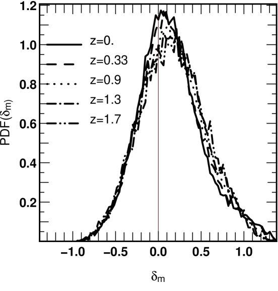
Figure 5: Top: Normalized probability distributions (PDF) of the excess of equatorial infall, $\delta_{m}$, measured at the virial radius. The quantity $1+\delta_{m}$ stands for the ratio between the flux of matter through the equatorial sub-region of the $R_{200}$ sphere and the average flux of matter through the whole $R_{200}$ sphere. The equatorial sub-region is defined as being perpendicular to the direction of the halo’s spin. It formally corresponds to the top-hat-smoothed mass flux density contrast. $\delta_{m}=0$ is expected for an isotropic infall of matter through the virial sphere. The average value of $\delta_{m}$ is always greater than 0 indicating that the infall of matter is, on average, more important in the direction orthogonal to the halo’s spin vector than in other directions. Bottom: the antisymmetric part of the $\delta_{m}$ distribution. Being positive for positive values of $\delta_{m}$, the antisymmetric part of the $\delta_{m}$ distributions shows that accretion in the equatorial plane is in excess relative to the one expected from an isotropic accretion of matter.

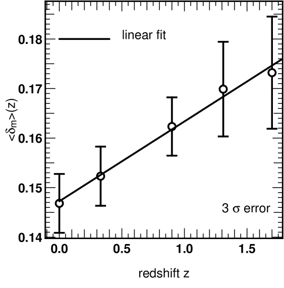
Figure 6: The redshift evolution of $\langle\delta_{m}\rangle$. The average $\langle\cdot\rangle$ is performed on a set of 40 000 haloes at $z=0$ and 10 500 haloes at $z=1.8$. The error bars stand for the error on the estimation of $\langle\delta_{m}\rangle$ with $\Delta=\sigma(\delta_{m})/\sqrt{N}$. N is the number of haloes needed to compute $\langle\delta_{m}\rangle$. $\langle\delta_{m}\rangle$ is always positive and indicates an excess of accretion in the equatorial plane. This redshift evolution can be fitted as $\langle\delta_{m}\rangle(z)=0.0161(\pm 0.0103)z+0.147(\pm 0.005)$. This excess is detected for every redshift smaller than $z=2$, which indicates an excess of accretion in the equatorial region. We applied a mass threshold of $5\cdot 10^{12}M_{\odot}$ to our haloes for every redshift. Then, the halo population is different from one redshift to another. This selection effect may dominate the observed time evolution.

The previous measurement doesn’t account for dark matter falling into the halo with a very small angular momentum (radial orbits). We therefore measured the excess of equatorial accretion, $\delta_{m}$, defined as follow. We can measure the average flow density of matter, $\Phi_{r}$, in a ring centered on the equatorial plane:

$$\Phi_{r}\equiv\frac{1}{S_{r}}\int_{-\pi/8<\theta-\pi/2<\pi/8}\rho{\bf v_{r}}({\mbox{\boldmath$\Omega$}})\cdot{{\mathrm{d}}}{{\mbox{\boldmath$\Omega$}}},$$ (14)

where $S_{r}=\int_{-\pi/8<\theta-\pi/2<\pi/8}{{\mathrm{d}}}{{\mbox{\boldmath$\Omega$}}}$. The ring-region is defined by the area where the polar angle satisfies $\theta_{pol}=\pi/2\pm\pi/8$ which corresponds to about 40 $\%$ of the total covered solid angle. The larger this region is, the better the convergence of the average value of $\Phi_{r}$, but the lower the effects of anisotropy, since averaging over a larger surface leads to a stronger smoothing of the field. This value of $\pm\pi/8$ is a compromise between these two contradictory trends. In the next section and in the appendix, we discuss more general filtering involving spherical harmonics which are related to the dynamical evolution of the inner component of the halo. We also measure the flow averaged on all the directions $\overline{\Phi}$:

$$\overline{\Phi}\equiv\overline{\rho{\bf v_{r}}}\equiv\frac{1}{4\pi}\int_{4\pi}\rho{\bf v_{r}}({\mbox{\boldmath$\Omega$}})\cdot{{\mathrm{d}}}{{\mbox{\boldmath$\Omega$}}}.$$ (15)

Since we are interested in accretion, we computed $\Phi_{r}$ and $\overline{\Phi}$ using only the infalling part of the density flux of matter, where $\rho{\bf v_{r}}({\mbox{\boldmath$\Omega$}})\cdot{{\mathrm{d}}}{{\mbox{\boldmath$\Omega$}}}<0$, ignoring the outflows. We therefore define $\delta_{m}$ as

$$\delta_{m}\equiv\frac{\Phi_{r}-\overline{\Phi}}{\overline{\Phi}}.$$ (16)

This number quantifies the anisotropy of the infall. It is positive when infall is in excess in the galactic-equatorial plane, while for isotropic infall $\delta_{m}\equiv 0$. The quantity $\delta_{m}$ can be regarded as being the ‘flux density’ contrast of the infall of matter in the ring region (formally it is the centered top-hat-filtered mass flux density contrast as shown in appendix C.1). This measurement, in contrast to those of the previous section does not rely on some knowledge on the inner region of the halo but only on the properties of the environment.

Fig. 5 displays the normalized distribution of $\delta_{m}$ measured for 50 000 haloes with a mass in excess of $5\cdot 10^{12}M_{\odot}$ and for different redshifts ($z=1.8,1.5,0.9,0.3,0.0$). The possible values for $\delta_{m}$ range between $\delta_{m}\sim-1$ and $\delta_{m}\sim 1.5$. The average value $\langle\delta_{m}\rangle$ of the distributions is statistically larger than zero (see also Fig. 6). Here $\langle\quad\rangle$ stands for the statistical expectation, which in this paper is approximated by the arithmetic average over many haloes in our simulations. The antisymmetric part of the distribution of $\delta_{m}$ is positive for positive $\delta_{m}$. The PDF of $\delta_{m}$ is skewed, indicating an excess of accretion through the equatorial ring. The median value for $\delta_{m}$ is $\delta_{\mathrm{med}}=0.11$, while the first $25\%$ haloes have $\delta_{m}<\delta_{25}\equiv-0.11$ and the first $75\%$ haloes have $\delta_{m}<\delta_{75}\equiv 0.37$. Therefore we have $(\delta_{75}-\delta_{\mathrm{med}})/(\delta_{25}-\delta_{\mathrm{med}})=1.13$, which quantifies how the distribution of $\delta_{m}$ is positively skewed. The skewness $S_{3}=\langle(\delta-{\bar{\delta}})^{3}\rangle/\langle(\delta-{\bar{\delta}})^{2}\rangle^{3/2}$ is equal to $0.44$. Combined with the fact that the average value $\langle\delta_{m}\rangle$ is always positive, this shows that the infall of matter is larger in the equatorial plane than in the other directions.

This result is robust with respect to time evolution (see Fig. 6). At redshift $z=1.8$, we have $\langle\delta_{m}\rangle=0.17$ which falls down to $\langle\delta_{m}\rangle=0.145$ at redshift $z=0$. This redshift evolution can be fitted as $\langle\delta_{m}\rangle(z)=0.0161(\pm 0.0103)z+0.147(\pm 0.005)$. This trend should be taken with caution. For every redshift z we take in account haloes with a mass bigger than $5\cdot 10^{12}M_{\odot}$. Thus the population of haloes studied at z=0 is not exactly the same as the one studied at z=2. Actually, at z=0, there is a strong contribution of small haloes (i.e. with a mass close to $5\cdot 10^{12}M_{\odot}$) which just crossed the mass threshold. The accretion on small haloes is more isotropic as shown in more details in appendix D.2. One possible explaination is that they experienced less interactions with their environment and have had since time to relax which implies a smaller correlation with the spatial distribution of the infall. Also bigger haloes tend to lie in more coherent regions, corresponding to rare peaks, whereas smaller haloes are more evenly distributed. The measured time evolution of the anisotropy of the infall of matter therefore seems to result from a competition between the trend for haloes to become more symmetric and the bias corresponding to a fixed mass cut.

In short, the infall of matter measured at the virial radius in the direction orthogonal to halo spin is larger than expected for an isotropic infall.

3.4 Harmonic expansion of anisotropic infall

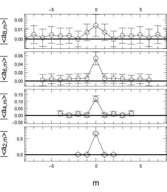
Figure 7: The convergence of modulus of the real part of $\langle{\tilde{a}_{\ell}^{m}}\rangle$, for $\ell=2,4,6,8$. The ${\tilde{a}_{\ell}^{m}}$ decomposition was computed for 25 000 haloes and each coefficient has been normalized with the corresponding $C_{0}$ (see text for details). Here, $\langle\,\,\,\rangle$ stands for the median while the error bars stand for the distance between the 5th and the 95th centile. The median value of $\langle\tilde{a}_{\ell}^{m}\rangle$ is zero except for the $\langle\tilde{a}_{\ell}^{0}\rangle$ coefficient: this is a signature of a field invariant to azimuthal rotations.

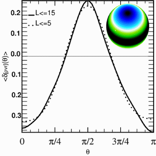
Figure 8: An illustration of the convergence of the $\tilde{a}_{\ell m}$ presented in Fig. 7. The solid line stands for the azimuthal average of the spherical contrast of accretion computed using Eq. (22). The dotted line for the spherical field reconstructed with $\ell\leq 5$. The insert represents the reconstructed spherical field using the expansion of the $\tilde{a}_{\ell m}$ of the mass flux measured at the virial sphere. The sphere presents an excess of accretion in the equatorial region because of the non-zero average value of $\tilde{a}_{\ell 0}$ coefficients (for even values of $\ell$).

As mentioned earlier (and demonstrated in appendix A), the dynamics of the inner halo and disk is partly governed by the statistical properties of the flux densities at the boundary. Accounting for the gravitational perturbation and the infalling mass or momentum requires projecting the perturbation over a suitable basis such as the spherical harmonics:

$$\varpi({\mbox{\boldmath$\Omega$}})=\sum_{\ell,m}\alpha^{m}_{\ell}Y_{\ell}^{m}({\mbox{\boldmath$\Omega$}})\,,$$ (17)

Here, $\varpi$ stands for, e.g. the mass flux density, the advected momentum flux density, or the potential perturbation. The resulting $\alpha_{\ell}^{m}$ coefficients correspond to the spherical harmonic decomposition in an arbitrary reference frame. The different $m$ correspond to the different fundamental orientations for a given multipole $\ell$. A spherical field with no particular orientation gives rise to a field averaged over the different realisations which appear as a monopole, i.e. $\langle\alpha_{\ell m}\rangle=0$ for $\ell\neq 0$. Having constructed our virial sphere in a reference frame attached to the simulation box, we effectively performed a randomization of the spheres’ orientation. However, since the direction of the halo’s spin is associated to a general preferred orientation for the infall, it should be traced through the $\alpha_{\ell m}$ coefficients. Let us define the rotation matrix, $\mathcal{R}$, which brings the z-axis of the simulation box along the direction of the halo’s spin. The spherical harmonic decomposition centered on the spin of the halo, $a_{\ell}^{m}$, is given by (e.g. Varshalovich et al. (1988)):

$$a^{m}_{\ell}=\mathcal{R}[\alpha^{m^{\prime}}_{\ell^{\prime}}]\equiv\sum_{\ell^{\prime}m^{\prime}}\mathcal{R}_{\ell,\ell^{\prime}}^{m,m^{\prime}}(\vartheta,\varphi)\alpha^{m^{\prime}}_{\ell^{\prime}}\,.$$ (18)

If the direction of the spin defines a preferential plane of accretion, the corresponding $a_{\ell}^{m}$ will be systematically enhanced. We therefore expect the equatorial direction (which corresponds to $m=0$ for every $\ell$) not to converge to zero.

We computed the spherical harmonic decomposition of $\rho v_{r}(\vartheta,\varphi)$ given by Eq. (17) for the mass flux density of 25 000 haloes at $z=0$, up to $\ell=15$. For each spherical field of the mass density flux, we performed the rotation that brings the halo’s spin along the z-direction to obtain a set of ‘centered’ $a_{\ell}^{m}$ coefficients. We also computed the related angular power spectrums $C_{\ell}$ :

$$C_{\ell}\equiv\frac{1}{4\pi}\frac{1}{2\ell+1}\sum_{m=-\ell}^{\ell}|a_{\ell}^{m}|^{2}=\frac{1}{4\pi}\frac{1}{2\ell+1}\sum_{m=-\ell}^{\ell}|\alpha_{\ell}^{m}|^{2}.$$ (19)

Let us define the normalized $\tilde{a}_{\ell}^{m}$ (or harmonic contrast, see appendix C.1),

$${\tilde{a}_{\ell}^{m}}\equiv\sqrt{4\pi}\frac{a_{\ell}^{m}}{a_{0}^{0}}=\frac{a_{\ell}^{m}}{\mathrm{sign}(a_{0}^{0})\sqrt{C_{0}}}.$$ (20)

This compensates for the variations induced by our range of masses for the halo. For each $\ell$, we present in Fig. 7 the median value, $|\langle\mathrm{Re}\left\{\tilde{a}_{\ell}^{m}\right\}\rangle|$ for $\ell=2,4,6,8$ computed for 25 000 haloes. All the $\tilde{a}_{\ell}^{m}$ have converged toward zero, except for the $\tilde{a}_{\ell 0}$ coefficients. The imaginary parts of $\tilde{a}_{\ell}^{m}$ have the same behaviour, except for the ${\rm Im}\{\tilde{a}_{\ell 0}\}$ coefficients which vanish by definition (not shown here). The $m=0$ coefficients are statistically non-zero. We find $\langle{\tilde{a}_{2}^{0}}\rangle=-0.65\pm 0.04$, $\langle{\tilde{a}_{4}^{0}}\rangle=0.12\pm 0.02$, $\langle{\tilde{a}_{6}^{0}}\rangle=-0.054\pm 0.015$ and $\langle{\tilde{a}_{8}^{0}}\rangle=0.0145\pm 0.014$. Errors stand for the distance between the 5th and the 95th centile. The typical pattern corresponding an $m=0$ harmonic is a series of rings parallel to the equatorial plane. This confirms that the accretion occurs preferentially in a plane perpendicular to the direction halo’s spin.

The spherical accretion contrast $\langle\delta_{\rho v_{r}}({\vartheta},\phi)\rangle$ can be reconstructed using the $\langle\tilde{a}_{\ell}^{m}\rangle$ coefficients (as shown in the appendix):

$$\delta_{[\rho v_{r}]}(\vartheta,\varphi)=\sum_{\ell,m}{\tilde{a}^{m}_{\ell}}Y_{\ell}^{m}(\vartheta,\varphi)-1.$$ (21)

In Fig. 8, the polar profile:

$$\langle\delta_{[\rho v_{r}]}({\vartheta})\rangle\equiv\sum_{\ell,m}\langle{\tilde{a}^{m}_{\ell}}\rangle Y_{\ell}^{m}(\vartheta,0)-1\,,$$ (22)

of this reconstructed spherical contrast is shown. This profile has been obtained using the $\langle\tilde{a}_{\ell}^{m}\rangle$ coefficients with $\ell\leq 5$ and $\ell\leq 15$. The contrast is large and positive near $\vartheta=\pi/2$ as expected for an equatorial accretion. The profile reconstructed using $\ell\leq 5$ is quite similar to the one using $\ell\leq 15$. This indicates that most of the energy involved in the equatorial accretion is contained in a typical angular scale of 36 degrees (a scale which is significantly larger than $\pi/20$ corresponding to the cutoff frequency in our sampling of the sphere as mentionned earlier).

Using a spherical harmonic expansion of the incoming mass flux density (Eq. (17)), we confirmed the excess of accretion in the equatorial plane found above. This similarity was expected since these two measurements (using a ring or using a spherical harmonic expansion) can be considered as two different filterings of the spherical accretion field as is demonstrated in the appendix C. The main asset of the harmonic filtering resides in its relevance for the description of the inner dynamics as is discussed in section 6.

3.5 Summary

To sum up, the two measurements of section 3.2 and 3.3 (or 3.4) are not sensitive to the same effects. The first measurement (involving the angular momentum $\rho{\bf L}$ at the virial radius) is mostly a measure of the importance of infalling matter in building the halo’s proper spin. The second and the third measurements (involving the excess of accretion in the equatorial plane, $\delta_{m}$, using rings and harmonic expansion) are quantitative measures of coplanar accretion. The equatorial plane of a halo is favoured relative to the accretion of matter (compared to an isotropic accretion) to a level of $\sim 12\%$ between $z=2$ and $z=0$. Down to the halo scale ($\sim 500$ kpc), anisotropy is detected and is reflected in the spatial configuration of infalling matter.

4 Anisotropic infall of substructures

To confirm and assess the detected anisotropy of the matter infall on haloes in our simulations, let us now move on to a discrete framework and measure related quantities for satellites and substructures. In the hierarchical scenario, haloes are built up by successive mergers of smaller haloes. Thus if an anisotropy in the distribution of infalling matter is to be detected it seems reasonable that this anisotropy should also be detected in the distribution of satellites. The previous galactocentric approach for the mass flow does not discriminate between an infall of virialised objects and a diffuse material accretion and therefore is also sensitive to satellites merging: one would need to consider, say, the energy flux density. However, it is not clear if satellites are markers of the general infall and Vitvitska et al. (2002) did not detect any anisotropy at a level greater than 20$\%$.

The detection of substructures and satellites is performed using the code ADAPTAHOP which is described in details in the appendix. This code outputs trees of substructures in our simulations, by analysing the properties of the local dark matter density in terms of peaks and saddle points. For each detected halo we can extract the whole hierarchy of subclumps or satellites and their characteristics. Here we consider the leaves of the trees, i.e. the most elementary substructures the haloes contain. Each halo contains a ‘core’ which is the largest substructure in terms of particles number and ‘satellites’ corresponding to the smaller ones. We call the ensemble core + satellites the ‘mother’ or the halo. Naturally the number of substructures is correlated with the mother’s mass. The bigger the number of substructures, the bigger the total mass. Because the resolution in mass of our simulations is limited, smaller haloes tend to have only one or two satellites. Thus in the following sections we will discriminate cases where the core have less than 4 satellites. A total of 50 000 haloes have been examined leading to a total of about 120 000 substructures.

4.1 Core spin - satellite orbital momentum correlations

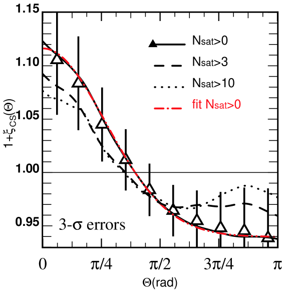
Figure 9: Excess probability, $1+\xi_{\mathrm{CS}}(\theta_{\rm cs})$, of the angle between the core’s spin and the orbital momentum of satellites. Cores have at least 1 satellite (solid line), 4 satellites (dashed line) and 10 satellites (dotted line). These curves have been normalized by the expected isotropic distribution and the Gaussian correction was applied to account for errors on the angle determination. Here $\xi_{\mathrm{CS}}(\theta)=0$ is expected for an isotropic distribution of angles between the core ’s spin and the orbital momentum. All satellites are external to the core, yet an excess of alignment is present. The triangles represent the angle distribution, the error bars stand for the $3\sigma$-dispersion for 50 subsamples of 10 000 satellites (out of 35 000) while the red curve stands for the best gaussian fit of the distribution for systems with at least one satellite (see Eq. 12 for parameterization). The best fit parameters are: $a_{1}=0.3993\pm 0.0038,a_{2}=0.0599\pm 0.0083,a_{3}=0.8814\pm 0.0055,a_{4}=0.9389\pm 0.0002$. The isotropic case is excluded with a good confidence level, even for systems with a large number of satellites.

In the mother-core-satellite picture, it is natural to regard the core as the central galactic system, while satellites are expected to join the halo from the intergalactic medium. One way to test the effect of large scale anisotropy is to directly compare the angle between the core’s spin, ${\bf S}_{c}$, and the satellites’ angular momentum, ${\bf L}_{s}$, relative to the core. These two angular momenta are chosen since they should be less correlated with each other than e.g. the haloes’ spin and the angular momentum of its substructures. Furthermore, particles that belong to the cores are strictly distinct from those that belong to satellites, thus preventing any ‘self contamination’ effect. As a final safeguard, we took in account only satellites with a distance relative to the core larger than the mother’s radius. The core’s spin is:

$${\bf S}_{c}=\sum_{p}({\bf r_{p}-r_{c}})\times({\bf v_{p}-v_{c}}),$$ (23)

where $\bf r_{p}$ and $\bf v_{p}$ (resp. $\bf r_{c}$ and $\bf v_{c}$) stands for particles’ position and velocities (resp. the core’s centre of mass position and velocity) and where:

$$r_{p}<d_{c},$$ (24)

where $d_{c}$ is the core’s radius. The angular momentum for a satellite is computed likewise, with a different selection criterion on particles, namely:

$$|{\bf r_{p}-r_{s}}|<d_{s},$$ (25)

where $\bf r_{s}$ stands for the satellite’s centre of mass position and $d_{s}$ is its radius.

Fig. 9 displays the reduced distribution of the angle, $\theta_{\rm cs}$, between the core’s spin and the satellites’ orbital momentum, where $\theta_{\rm cs}$ is defined by:

$$\theta_{\rm cs}=\cos^{-1}(\frac{{\bf L}_{s}\cdot{\bf S}_{c}}{|{\bf L}_{s}||{\bf S}_{c}|}).$$ (26)

The Gaussian correction was applied as described in section 3.2, to take into account the uncertainty on the determination of $\theta_{\rm cs}$.

The correlation of $\theta_{\rm cs}$ indicates a preference for the aligned configuration with an excess of $\sim 12\%$ of aligned configurations relative to the isotropic distribution. We ran Monte-Carlo realisations using 50 subsamples of 10 000 haloes extracted from our whole set of substructures to constrain the error bars. We found a $3\sigma$ error of $6\%$: the detected anisotropy exceeds our errors, i.e. $\xi_{\mathrm{CS}}(\theta_{\rm cs})$ is not uniform with a good confidence level. The variations with the fragmentation level (i.e. the number of satellites per system) remains within the error bars. The best fit parameters for the measured distributions of systems with at least 1 satellite are $a_{1}=0.3993\pm 0.0038,a_{2}=0.0599\pm 0.0083,a_{3}=0.8814\pm 0.0055,a_{4}=0.9389\pm 0.0002$ (see Eq. 12 for parametrization). Not surprisingly, a less structured system shows a stronger alignment of its satellites’ orbital momentum relative to the core’s spin. In the extreme case of a binary system (one core plus a satellite), it is common for the two bodies to have similar mass. Since the two bodies are revolving around each other, a natural preferential plane appears. The core’s spin will be likely to be orthogonal to this plane. Increasing the number of satellites increases the isotropy of the satellites’ spatial distribution (the distributions maxima are lower and the slope toward low values of $\theta_{\rm cs}$ is gentler), but switching from at least 4 satellites to at least 10 satellites per system does not change significantly the overwhole shape distribution. This suggests that convergence, relative to the number of satellites, has been reached for the $\theta_{\rm cs}$ distribution.

As the measurements of the anisotropy factor $\delta_{m}$ indirectly suggested, satellites have an anisotropic distribution of their directions around haloes. Furthermore the previous analysis of the statistical properties of $\delta$ (section 3.3) indicated an excess of aligned configuration of $15\%$ which is consistent with the current method using substructures. While the direction of the core’s spin should not be influenced by the infall of matter, we still find the existence of a preferential plane for this infall, namely the core’s equatorial plane.

4.2 Satellite velocity - satellite spin correlation

The previous sections compared haloes’ properties with the properties of satellites. In a galactocentric framework, the existence of this preferential plane could only be local. In the extreme each halo would then have its own preferential plane without any connection to the preferential plane of the next halo. Taking the satellite itself as a reference, we have analyzed the correlation between the satellite average velocity in the core’s rest frame and the structures’ spin. Since part of the properties of these two quantities are consequences of what happened outside the galactic system, the measurement of their alignment should provide information on the structuration on scales larger than the haloes scales, while sticking to a galactocentric point of view.

For each satellite, we extract the angle, $\theta_{\rm vs}$, between the velocity and the proper spin and derive its distribution using the Gaussian correction (see fig. 10). The satellite’s spin ${\bf S}_{s}$ is defined by:

$${\bf S}_{s}=\sum_{p}({\bf r_{p}-r_{s}})\times({\bf v_{p}-v_{s}}),$$ (27)

where $\bf r_{s}$ and $\bf v_{s}$ stands for the satellite’s position and velocity in the halo core’s rest frame. The angle, $\theta_{\mathrm{vs}}$, between the satellite’s spin and the satellite’s velocity is:

$$\theta_{\mathrm{vs}}=\cos^{-1}(\frac{{\bf S}_{s}\cdot{\bf v}_{s}}{|{\bf S}_{s}||{\bf v}_{s}|}).$$ (28)

Only satellites external to the mother’s radius are considered while computing the distribution of angles. This leads to a sample of about 40 000 satellites, at redshift $z=0$. The distribution $\xi(\theta_{\rm vs})$ was calculated as sketched in section 2. An isotropic distribution of $\theta_{\rm vs}$ would as usual lead to a uniform distribution $\xi(\theta_{\rm vs})=0$. The result is shown in Fig. 10. The error bars were computed using the same Monte-Carlo simulations described before with 50 subsamples of 10 000 satellites.

We obtain a peaked distribution with a maximum for $\theta_{\rm vs}=\pi/2$ corresponding to an excess of orthogonal configuration of $5\%$ compared to a random distribution of satellite spins relative to their velocities. The substructures’ motion is preferentially perpendicular to their spin. This distribution of angles for systems with at least 1 satellite can be fitted by a Gaussian function with the following best fit parameters (see Eq 12): $a_{1}=0.2953\pm 0.0040,a_{1}=1.5447\pm 0.0015,a_{2}=0.8045\pm 0.0059,a_{3}=0.9144\pm 0.0010$. The variation with the mother’s fragmentation level is within the error bars. However the effect of an accretion orthogonal to the direction of the spin is stronger for satellites which belong to less structured systems. This may be again related to the case where two comparable bodies revolve around each other, but from a satellite point-of-view. The satellite spin is likely to be orthogonal to the revolution plane and consequently to the velocity’s direction.

This result was already known for haloes in filaments (Faltenbacher et al. (2002)), where their motion occurs along the filaments with their spins pointing outwards. The current results show that the same behaviour is measured down to the satellite’s scale. However this result should be taken with caution since Monte-Carlo tests suggest that the error (deduced from the $3\sigma$ dispersion) is about $4\%$.

This configuration where the spins of haloes and satellites are orthogonal to their motion fit with the image of a flow of structures along the filaments. Larger structures are formed out of the merging of smaller ones in a hierarchical scenario. Such small substructures should have small relative velocities in order to eventually merge while spiraling towards each other. The filaments correspond to regions where most of the flow is laminar, hence the merging between satellites is more likely to occur when one satellite catches up with another, while both satellites move along the filaments. During such encounter, shell crossing induces vorticity perpendicular to the flow as was demonstrated in Pichon & Bernardeau (1999). This vorticity is then converted to momentum, with a spin orthogonal to the direction of the filament.

Finally, the flow of matter along the filaments may also provide an explanation for the excess of accretion through the equatorial regions of the virial sphere. If a sphere is embedded in a ‘laminar’ flow, the density flux detected near the poles should be smaller than that detected near the ‘equator’ of the sphere. The flux measured on the sphere is larger in regions where the normal to the surface is collinear with the ‘laminar’ flow, i.e. the ‘equator’. On the other hand, a nil flux is expected near the poles since the vector normal to the surface is orthogonal to direction of the flow. The same effect is measured on Earth which receives the Sun radiance: the temperature is larger on the Tropics than near the poles. Our observed excess of accretion through the equatorial region supports the idea of a filamentary flow orthogonal to the direction of the halo’s spin down to scales $\leq 500$ kpc.

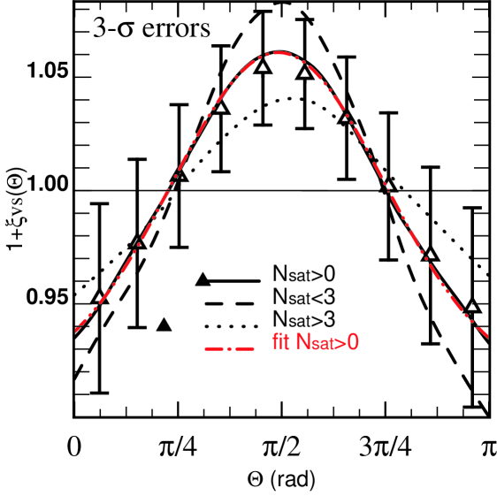
Figure 10: Excess probability, $1+\xi_{\mathrm{vs}}$, of the angle between the substructures’ spin and their velocities in the mother’s rest frame. The Gaussian correction was applied to take into account uncertainty on the angle determination. The distributions was measured for all mothers (solid), mothers with at least 4 substructures (dot) and mothers with at most 3 substructures (dash). The triangles represent the mean angle distribution. The error bars represent the Monte Carlo $3\sigma$-dispersion for 50 subsamples of 10 000 haloes (out of 35 000). The red dash-dotted curve stands for the best fit of the distribution with a Gaussian function for systems with at least 1 satellite (see Eq. 12 for parametrization). The best fit parameters are: $a_{1}=0.2953\pm 0.0040,a_{1}=1.5447\pm 0.0015,a_{2}=0.8045\pm 0.0059,a_{3}=0.9144\pm 0.0010$. In the core’s rest frame, the satellites’ motion is orthogonal to the direction of the satellites’ spin. This configuration would fit in a picture where structures move along filamentary directions.

5 Projected anisotropy

5.1 Projected satellites population

We looked directly into the spatial distributions of satellites surrounding the haloes cores to confirm the existence of a preferential plane for the satellites locations in projection. In Fig. 11, we show the compilation of the projected positions of satellites in the core’s rest frame. The result is a synthetic galactic system with 100 000 satellites in the same rest frame. We performed suitable rotations to bring the spin axis collinear to the z-axis for each system of satellites, then we added all these systems to obtain the actual synthetic halo with 100 000 satellites. The positions were normalized using the mother’s radius (which is of the order of the virial radius). A quick analysis of the isocontours of the satellite distributions indicates that satellites are more likely to be found in the equatorial plane, even in projection. The axis ratio measured at one mother’s radius is $\epsilon(R_{m})\equiv a/b-1=0.1$ with $a>b$. We compared this distribution to an isotropic ‘reference’ distribution of satellites surrounding the core. This reference distribution has the same average radial profile as the measured satellite distributions but with isotropically distributed directions. The result of the substraction of the two profiles is also shown in Fig. 11. The equatorial plane (perpendicular to the z-axis) presents an excess in the number of satellites (light regions). Meanwhile, there is a lack of satellites along the spin direction (dark regions). This confirms our earlier results obtained using the alignment of orbital momentum of satellites with the core’s spin, i.e. satellites lie more likely in the plane orthogonal to the halo spin direction. Qualitatively, these results have already been obtained by Tormen (1997), where the major axis of the ellipsoid defined by the satellite’s distribution is found to be aligned with the cluster’s major axis. This synthetic halo is more directly comparable to observables since, unlike the dark matter halo itself, the satellites should emit light. Even though $\Lambda$CDM predicts too many satellites, its relative geometrical distribution might still be correct. In the following sections, our intent is to quantify more precisely this effect.

The propension of satellites to lie in the plane orthogonal to the direction of the core’s spin appears as an ‘anti-Holmberg’ effect. Holmberg (1974) and more recently Zaritsky et al. (1997) have found observationnally that the distribution of satellites around disks is biased towards the pole regions. Thus if the orbital momentum vector of galaxies is aligned with the spin of their parent haloes, our result seems to contradict these observations. One may argue that satellites are easier to detect out of the galactic plane. Furthermore our measurements are carried far from the disk while its influence is not taken in account. Huang & Carlberg (1997) have shown that the orbital decay and the disruption of satellites are more efficient for coplanar orbits near the disk. It would explain the lack of satellites in the disk plane. Thus our distribution of satellites can still be made consistent with the ‘Holmberg effect’.

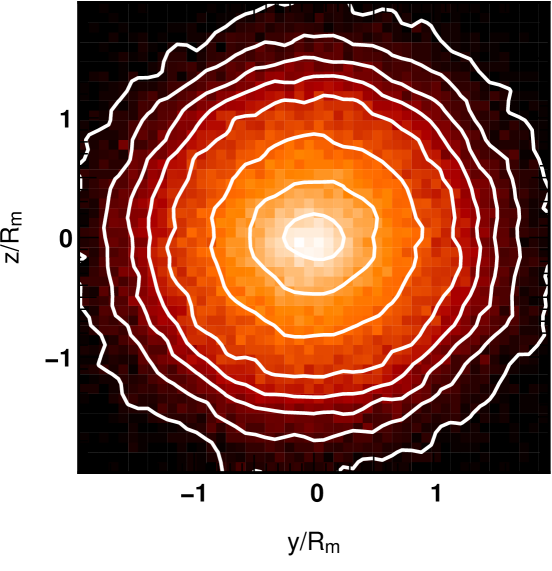
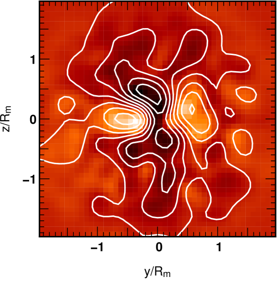
Figure 11: The projected distribution of satellites around the core’s centre of mass. We used the position of 40 000 satellites around their respective core to produce a synthetic halo+satellites (a ‘mother’) system. The projection is performed along the x-axis. The y and z coordinates are given in units of the mother’s radius. The z-axis is colinear to the direction of the core’s spin. Top: The isocontours of the number density of satellites around the core’s centre of mass present a flattened shape. The number of satellites is lower in darker bins than in lighter bins. The flattened isocontours indicate that satellites lie preferentially in the plane orthogonal to direction of the spin. Bottom: The excess number of satellites surrounding the core. We compared the distribution of satellites measured in our simulations to an isotropic distribution of satellites. Light zones stand for an excess of satellites in these regions (compared to an isotropic distribution) while dark zones stand for a lack of satellites. The satellites are more numerous in the equatorial region than expected in an isotropic distribution of satellites around the core. Also, there are fewer satellites along the spin’s axis than expected for an isotropic distribution of satellites.

5.2 Projected satellite orientation and spin

In addition to the known alignment on large scales, we have shown that the orientation of structures on smaller scales should be different from the one expected for a random distribution of orientations. Can this phenomenon be observed ? The previous measurements were carried in 3D while this latter type of observations is performed in projection on the sky. The projection ‘dilutes’ the anisotropy effects detected using three-dimensional information. Thus an effect of $15\%$ may be lowered to a few percents by projecting on the sky. However, even if the deviation from isotropy is as important as a few percents, as we will suggest, this should be relevant for measurements involved in extracting a signal just above the noise level, such as weak lensing.

To see the effect of projection on our previous measurements, we proceed in two steps. First, every mother (halo core + satellites) is rotated to bring the direction of the core’s spin to the z-axis. Second, every quantity is computed using only the y and z components of the relevant vectors, corresponding to a projection along the x-axis.

The first projected measurement involves the orientation of satellites relative to their position in the core’s rest frame. The spin of a halo is statistically orthogonal to the main axis of the distribution of matter of that halo (Faltenbacher et al. (2002)), and assuming that this property is preserved for satellites, their spin $\bf S_{s}$ is an indicator of their orientation. The angle, $\theta_{\rm P}$ (in projection), between the satellites’ spin and their position vector (in the core’s rest frame) is computed as follow:

$$\theta_{\mathrm{P}}=\cos^{-1}(\frac{{\bf S}_{s}^{y,z}\cdot{\bf r}_{sc}^{y,z}}{|{\bf S}_{s}^{y,z}||{\bf r}_{sc}^{y,z}|}),$$ (29)

with

$${\bf r}_{sc}={\bf r}_{s}-{\bf r}_{c},$$ (30)

where ${\bf r}_{s}$ and ${\bf r}_{c}$ stand respectively for the position vector of the satellite and the core’s centre of mass. Two extreme situations can be imagined. The ‘radial’ configuration corresponds to a case where the satellite’s main axis is aligned with the radius joining the core’s centre of mass to the satellite centreof mass (spin perpendicular to the radius, or $\theta_{\rm P}\sim\pi/2$). The ‘circular’ configuration is the case where the satellite main axis is orthogonal to the radius (spin parallel to the radius, $\theta_{\rm P}\sim 0[\pi]$). These reference configuration will be discussed in what follows.

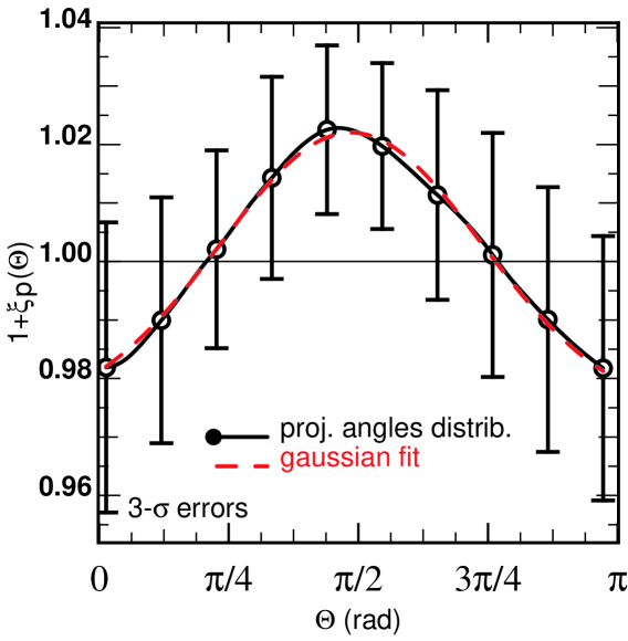
Figure 12: Excess probability, $1+\xi_{P}$, of the projected angles between the direction of the spin of substructures and their position vector in the core’s rest frame . The projection is made along the x-axis where the z-axis is concurrent with the core’s spin direction. The solid line represents the average distribution of projected angles of 50 subsamples of 50 000 substructures (out of 100 000 available substructures). The error bars represents the $3\sigma$ -dispersion relative to these 50 subsamples. An isotropic distribution of orientation would correspond to a value of 1 for $1+\xi_{\rm P}$. The projection plus the reference to the position vector instead of the velocity’s direction lowers the anisotropy effect. The red curve stands for the best Gaussian fit of the excess probability (see Eq. 12 for parameterization). The best fit parameters are: $a_{1}=0.0999\pm 0.0030,a_{2}=1.5488\pm 0.0031,a_{3}=0.8259\pm 0.0131,a_{4}=0.9737\pm 0.0007$. It seems that on average the projected orientation of a substructure is orthogonal to its projected position vector.

The resulting distribution, $1+\xi_{\rm P}(\theta_{\rm P})$, is shown in Fig. 12. As before, an isotropic distribution of orientations would lead to $\xi_{\rm P}(\theta_{\rm P})=0$. The distribution is computed with 100 000 satellites, without the cores, while the error bars result from Monte-Carlo simulations on 50 subsamples of 50 000 satellites each. As compared to the distribution expected for random orientations, the orthogonal configuration is present in excess of $\xi_{\rm P}(\pi/2)\sim 0.02$. If the spin of satellites is orthogonal to their principal axis, the direction vector in the core’s rest frame is more aligned with the satellites principal axes than one would expect for an isotropic distribution of satellites’ orientations. This configuration is ‘radial’. The peak of the distribution is slightly above the error bars: $\Delta\xi_{\rm P}(\theta_{\rm P}\sim\pi/2)\sim 0.02$. The distribution can be fitted by the Gaussian function given in Eq. 12 with the following parameters: $a_{1}=0.0999\pm 0.0030,a_{2}=1.5488\pm 0.0031,a_{3}=0.8259\pm 0.0131,a_{4}=0.9737\pm 0.0007$. The alignment seems to be difficult to detect in projection. With 50 000 satellites, we barely detect the enhancement of the orthogonal configuration at the 3-$\sigma$ level, thus we do not expect a detection of this effect at the 1-$\sigma$ level for less than 6000 satellites. Nevertheless, the distribution of the satellites’ orientation in projection seems to be ‘radial’ on dynamical grounds, without reference to a lensing potential.

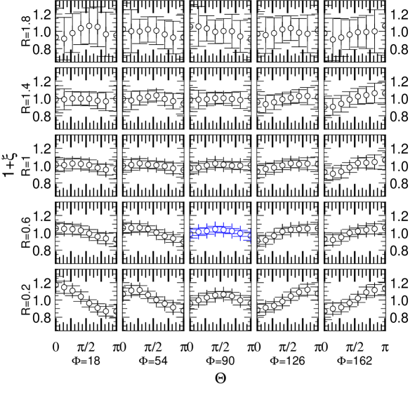
Figure 13: Radial and azimuthal grid of the excess probability, $1+\xi_{\rm P}$, of the projected angles between the direction of the spin of substructures and their direction relative to the central position of the core (as shown on average in Fig 12). The projection is made along the x-axis where the z-axis is concurrent with the direction of the core’s spin. Each row represents a distance relative to central core in the mother’s radius units (from bottom to top): $R\in[0,0.4[$, $R\in[0.4,0.8[$, $R\in[0.8,1.2[$, $R\in[1.2,1.6[$ and $R\in[1.6,2[$. Each column represents an angular distance (in degrees) relative to the direction of the core’s spin (z-axis) : $\phi_{s}\in]0,36]$, $\phi_{s}\in[36,72[$, $\phi_{s}\in[72,108[$, $\phi_{s}\in[108,144[$ and $\phi_{s}\in[144,180[$. The isotropic orientation distribution corresponds to a value of 1. Each sector presents a preferential direction that depends on its position relative to the spin direction of the central core. The distributions are computed using 50 samples of 50 000 satellites each. In each sector, the points represents the distribution averaged over the 50 samples. The error bars represent the $3\sigma$-Monte Carlo dispersion of the distribution over these 50 samples.

Figure 14: Geometric configuration of mean satellites around their core galaxy; each panel of Fig. 13 is represented by an ellipse at its log radius and angle around the core galaxy. The axis ratio of the ellipses is proportional to the peak-to-peak amplitude of the corresponding correlation (accounting for the relative SNR), while its orientation is given by the orientation of the maximum of $1+\xi_{\rm P}$.

Our previous measurement was ‘global’ since it does not take into account the possible change of orientation with the relative position of the satellites in the core’s rest frame. In Fig. 13, we explore the evolution of $1+\xi_{\rm P}$ with the radial distance relative to the core’s centre of mass and with the angular distance relative to the z-axis, i.e. relative to the direction of the core’s spin. The previous synthetic halo was divided in sectors and for each sector, $1+\xi_{\rm P}$ can be computed. The sectors are thus defined by their radius (in the mother’s radius units): $R\leq 0.4$, $0.4<R\leq 0.8$, $0.8<R\leq 1.2$, $1.2<R\leq 1.6$ and $1.6<R\leq 2$ and by their polar angle relative to the direction of the core’s spin (in degrees): $\phi_{s}\leq 36$, $36<\phi_{s}\leq 72$, $72<\phi_{s}\leq 108$, $108<\phi_{s}\leq 144$ and $144<\phi_{s}\leq 180$. Each of the previous Monte-Carlo subsamples can also be divided into sectors in order to compute the dispersion $\sigma$ for the distributions within the subsamples. The error bars still represent the $3\sigma$ dispersions.

The Fig. 14 is a qualitative representation of the results presented in Fig. 13. Each sector with $R\leq 1$ in Fig. 13 is represented by an ellipse at its actual position. The orientation of the ellipse is given by the angle of the maximum of the corresponding $1+\xi_{\rm P}(\theta_{p})$ function. We chose to represent the spin’s direction perpendicular to the ellipse’s major axis. We also chose to scale the ellipse axis ratio with the signal-to-noise ratio of $1+\xi_{\rm P}(\theta_{p})$. Indeed large errors leads to weak constrains on the spin orientation and the galaxy would be seen as circular on average. Conversely a strongly constrained orientation leads to a typical axis ratio of 0.5.

Two effects seem to emerge from this investigation. For some sectors, the orthogonal configuration is in excess compared to an isotropic distribution of satellites’ orientation relative to the radial vector. This seems to be true especially for radii smaller than the mother’s radius but the effect is still present at larger distances, especially near $\phi_{s}\sim\pi/2$. Switching from low values to high values of $\phi_{s}$ changes the slope of the $1+\xi_{\rm P}(\theta)$ distribution. This may be a marker of a ‘circular configuration’ of the orientation of satellites.

The existence of a ‘radial’ component in the orientation of the satellites was expected, both from the unprojected measurements made in the previous sections and from the global distribution extracted from the projected data. The fact that the ‘radial’ signature is stronger around the equatorial plane ($72<\phi_{s}<108$ in Fig. 13) may be an another evidence for a filamentary flow of satellites, even in projection. It seems that the existence of a ‘circular’ component was mostly hidden in the previous measurements by the dominant signature of the ‘radial’ flow. Nevertheless, the dominance of ’circular’ orientations near the poles fits with the picture of a halo surrounded by satellites with their spin pointing orthogonally to the filament directions.

The ‘circular’ flow may alternatively be related to the flow of structures around clusters located at the connection between filaments. There are observations of such configurations (Kitzbichler $\&$ Saurer 2003), where galaxies have their spin pointing along their direction of accretion and these observations could be consistent with our ‘circular’ component.

6 Applications

Let us give here a quick overview of the implications of the previous measurements for the inner dynamics of the halo down to galactic scales. In particular let us see how the self-consistent dynamical response of the halo propagates anisotropic infall inwards, and then briefly and qualitatively discuss implications of anisotropy to galactic warps, disk thickening and lensing.

6.1 Linear response of galaxies

In the spirit of e.g. Kalnajs (1971) or Tremaine & Weinberg (1984) we show in appendix A and elsewhere (Aubert & Pichon (2004)) how to propagate dynamically the perturbation from the virial radius into the core of the galaxy using a self consistent combination of the linearized Boltzmann and Poisson equations under the assumption that the mass of the perturbation is small compared to the mass of the host galaxy. Formally, we have:

$${\mathbf{r}}({\mathbf{x}},t)={\mathbf{R}}[F,{\mbox{\boldmath$\Omega$}},{\mathbf{x}},t-\tau]\left({{\varpi}}({\mbox{\boldmath$\Omega$}},\tau)\right)\,,$$ (31)

where $\mathbf{R}$ is a linear operator which depends on the equilibrium state of the galactic halo (+disk) characterized by its distribution function $F$, and ${\mathbf{r}}({\mathbf{x}},t)$ represents the self consistent response of the inner halo at time t due to a perturbation ${{\varpi}}({\mbox{\boldmath$\Omega$}},\tau)$ occuring at time $\tau$. Here $\varpi$ represents formally the perturbed potential on the virial sphere and the flux density of advected momentum, mass and kinetic energy at $R_{200}$. A ‘simple’ expression for ${\mathbf{R}}$ is given in Appendix A for the self consistent polarisation of the halo. The linear operator, ${\mathbf{R}}$, follows from Eq. (42), (49) and  (52). These equations generalize the work of Kalnajs in that it accounts for a consistent infall of advected quantities at the outer edge of the halo. It is shown in particular in appendix A that self-consistency requires the knowledge of all ten (scalar, vector and symmetric tensor) fields $\varpi_{\rho}({{\mbox{\boldmath$\Omega$}}},\tau),\varpi_{\rho{\bf v}}({{\mbox{\boldmath$\Omega$}}},\tau),\varpi_{\rho\sigma_{i}\sigma_{j}}({{\mbox{\boldmath$\Omega$}}},\tau)$.

When dealing with disk broadening, ${\mathbf{r}}$ could be the velocity orthogonal to the plane of the disk, or, for the warp, its amplitude, as a function of the position in the disk, ${\mathbf{x}}$ (or the orientation of each ring if the warp is described as concentric rings). More generally, it could correspond to the perturbed distribution function of the disk+halo. The whole statistics of ${\mathbf{r}}$ is relevant. The average response $\langle{\mathbf{r}}({\mathbf{x}},t)\rangle$ can be written as:

$$\langle{\mathbf{r}}({\mathbf{x}},t)\rangle={\mathbf{R}}\langle\varpi({\mbox{\boldmath$\Omega$}},\tau)\rangle=\sum_{\ell m}{\mathbf{R}}Y_{\ell}^{m}({\mbox{\boldmath$\Omega$}})\langle a^{m}_{\ell}\rangle$$ (32)

Since the accretion is anisotropic, $\langle a^{m}_{\ell}\rangle$ do not converge toward zero (see section 3.4) inducing a non-zero average response. Most importantly the two point correlation of the response since it will tell us qualitatively what the correlation length and the root mean square amplitude of the response will be. For the purpose of this section, and to keep things simple, we will ignore temporal issues (discussed in Appendix A) altogether, both for the mean field and the cross-correlations. The two-point correlation of ${\mathbf{r}}({\mathbf{x}})$ then depends linearly on the two-point correlation of ${\varpi}$:

$$\langle{{\mathbf{r}}({\mathbf{x}})}\cdot{{\mathbf{r}}^{\top}}({\mathbf{y}})\rangle={\mathbf{R}}\langle{{\varpi}}({\mbox{\boldmath$\Omega$}})\cdot{{{\varpi}}^{\top}}({\mbox{\boldmath$\Omega$}}^{\prime})\rangle{{{\mathbf{R}}}^{\top}}\,,$$ (33)

where ^⊤ stands for the transposition. Clearly, if the infall, $\varpi({\mbox{\boldmath$\Omega$}}$), is anisotropic the response will be anisotropic. As was discussed in section 3.4 when the infall is not isotropic, we have

$$\langle|\tilde{a}^{m}_{\ell}|^{2}\rangle\neq\langle|\tilde{\alpha}^{m}_{\ell}|^{2}\rangle=\frac{1}{2\ell+1}\sum_{m=-\ell}^{m=\ell}\langle|\tilde{\alpha}^{m}_{\ell}|^{2}\rangle\,,$$ (34)

Let us therefore introduce:

$$\Delta\tilde{R}_{\ell}^{m}\equiv\langle|\tilde{a}^{m}_{\ell}|^{2}\rangle-\langle|\tilde{\alpha}^{m}_{\ell}|^{2}\rangle,$$ (35)

which would be identically zero if the field were stationary on the sphere. Here $\Delta\tilde{R}_{\ell}^{m}$ represents the anisotropic excess for each harmonic correlation. In particular, the excess polarisation of the response induced by the anisotropy reads

$$\Delta\langle{{\mathbf{r}}({\mathbf{x}})}\cdot{{\mathbf{r}}^{\top}}({\mathbf{y}})\rangle=\sum_{\ell m}{\mathbf{R}}Y_{\ell}^{m}({\mbox{\boldmath$\Omega$}})\Delta\tilde{R}_{\ell}^{m}Y_{\ell}^{m}({\mbox{\boldmath$\Omega$}}^{\prime}){{\mathbf{R}}^{\top}}\,.$$ (36)

Fig. 15 displays $\Delta\tilde{R}_{\ell}^{m}$, for $\ell=1,2,3,4$. The different $\Delta\tilde{R}_{\ell}^{m}$ clearly converge toward different non-zero values. Consequently the response should reflect the anisotropic nature of the external perturbations.

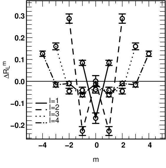
Figure 15: The residual anisotropic harmonic power spectra, $\Delta\tilde{R}_{\ell}^{m}$, introduced in Eq. (35) as a function of $m$ for $\ell=1,2,3,4$. These residuals will serve as input to the computation of the dynamical response of the halo.

It is beyond the scope of this paper to pursue the quantitative exploration of the response of the inner halo to a given anisotropic infall, since this would require an explicit expression of the response operator, ${\mathbf{R}}$, for each dynamical problem investigated.

6.2 Implication for warps, thick disks and lensing

In this paper, the main emphasis is on measured anisotropies. It turns out that it never exceeds 15 $\%$ in accretion. For a whole class of dynamical problems where anisotropy is not the dominant driving force it can be ignored at that level. Here we now discuss qualitatively the implication of the previous measurements to galactic warps, the thick disk and weak lensing where anisotropy is essential.

6.2.1 Galactic warps

The action of the torque applied on the disk of a galaxy is different for different angular and radial position of the perturbation. Consequently the warp’s orientation and its amplitude are functions of the spatial configuration of the external potential. For example, López-Corredoira et al. (2002) found that the warp’s amplitude due to an intergalactic flow is dependent on the direction of the incoming ‘beam’ of matter. Having modelled the intergalactic flow applied to the Milky Way, they found that the warp amplitude rises steeply as the beam leaves the region coplanar to the disk and this warp amplitude reaches a maximum for an inclination of 30 degrees relative to the disk’s plane. As the beam direction becomes perpendicular to the galactic plane, the warp amplitude decreases slowly. In this context, the existence of a typical spatial configuration for the incoming intergalactic matter or satellites infall may induce a kind of ’typical’ warp in the disk of galaxies.

The existence of a preferential plane for the accretion of angular momentum also implies that the recent evolution of the halo’s spin has been rather smooth. Bullock et al. (2001) have shown that the angular momentum tends to remain aligned within haloes. Furthermore, the accretion of matter by haloes is preferentially performed on plunging radial orbits, thus the inner parts of haloes are aware of the properties of the recently accreted angular momentum. Therefore, a disk embedded in the halo would also ‘feel’ this anisotropic accretion. Ostriker & Binney (1989) have shown that the misalignment of the accreted angular momentum and the disk’s spin forces the latter to slew the symmetry axis of its inner parts. The warp line of nodes is also found to be aligned with the axis of the torque applied to the disk. As stressed by Binney (1992), non straight line of nodes can be associated with changes in the direction of the accreted angular momentum. Using a sample of 12 galaxies, Briggs (1990) established rules of thumb for galactic warps, one of them being that the line of nodes is straight in the inner region of disk while it is wound in the outer parts. If the angular momentum is accreted along a stationary preferential direction, as we suggest, the warp line of nodes should remain mostly straight. However, if the accretion plane differs slightly from the disk plane, more than one direction of accretion become possible (by symmetry around the vector defining the disk plane) and, as a consequence, different directions are possible for the torque induced by accreted matter. We may then consider a varying torque along accretion history with an accreted angular momentum ‘precessing’ around the halo’s spin but close to its direction. In this scenario, the difference in the behaviour of the warp line of nodes between the inner and outer regions of the galaxies may be explained.

6.2.2 Galactic disk thickening

Thin galactic disks put serious constraints on merging scenarii, since their presence implies a fine-tuning between the cooling mechanisms (e.g. coplanar infall of gas), and the heating processes (merging of small virialised objects, deflection of spirals on molecular clouds). It has been shown that small mergers can produce a thick disk (e.g. Quinn et al. (1993), Walker et al. (1996) ). However, the presence of old stars within the thin disk cannot be explained in the framework of the merging scenario unless a fraction of the accretion took place within the equatorial plane of the galaxy. Furthermore, the geometric characteristic of the infall is essential in the formation process of a thick disk. In Velazquez & White (1999), numerical simulations of interactions between galactic disks and infalling satellites show that the heating and thickening is more efficient for coplanar satellites. They also stressed the differences between the effect of prograde or retrograde orbits of infalling satellites (relative to the rotation of the disk): prograde orbits induce disk heating while retrograde orbits induce disk tilting. Our results indicate that the infall is preferentially prograde and coplanar relative to the halo’s spin: if we consider an alignment between the halo’s spin and the galaxy’s angular momentum, the thickening process may be more efficient than the one expected in an isotropic configuration of infalling matter. Furthermore, our estimate of the fraction of coplanar accretion at the virial scale may be considered as a lower bound near the disk since the presence of a disk will focus the infall closer to the galactic plane. In fact, Huang & Carlberg (1997) found that the disk tends to tilt toward the orbital plane of infalling prograde low-density satellites. This effect would also contribute to enhance the excess of coplanar accretion down to galactic scales.

However the nature of infalling virialised objects was shown to affect their ability to heat or destroy the disk. Huang & Carlberg (1997) found that the presence of low density satellites should induce preferentially a tilting of the disk instead of a thickening: one needs to enhance the relative mass of the satellite ($\sim 30\%$ of the disk mass) to produce an observable thickening in the inner parts of the galaxy. Unfortunately such a massive satellite has a destructive impact on the outer parts of the disk. The relationship between the excess of accretion and the satellite mass should be constrained but our limited mass resolution prevents us from performing such a quantitative analysis. We should therefore aim at achieving higher angular resolution of the virial sphere and higher mass resolution in order to describe well compact virialised objects.

6.2.3 Gravitational lensing

The first detection of cosmic shear was reported by four different groups in 2000 (Bacon et al. (2000), Kaiser et al. (2000), Van Waerbeke et al. (2000), Wittman et al. (2000)). One of the basic assumptions made by cosmic shear studies is that the intrinsic ellipticities of galaxies are expected to be uncorrelated, and that the observed correlations are the results of gravitational lensing induced by the large scale structures between those galaxies and the observer. Hence, the detection of weak lensing signal assumes a gravitationally induced departure from a random distribution of the galactic shapes. Consequently, if there exists intrinsic alignments or preferential patterns in galactic orientations, this would potentially affect the interpretation from weak lensing measurements. Several papers have already considered the ‘contamination’ of the weak lensing signal by intrinsic galactic alignment. Using analytic arguments, Catelan et al. (2001) have shown that such alignments should exist. The issue of the amplitude of the intrinsic correlations compared to the correlation induced by the cosmic shear has also been explored by Croft & Metzler (2000) and Heavens et al. (2000). The ‘intrinsic’ correlations may overcome the shear-induced signal in surveys with a narrow redshift range. We have shown that the orientation of satellites around haloes is not randomly distributed, which is a clear indication of intrinsic correlations for our considered scales ($\sim$ 500 kpc). Taking $z_{m}=1$ as a typical median redshift for large lensing surveys, the corresponding angular scale is 1 arcminute in our simulations’ cosmogony. Furthermore, the prospect of studying the redshift evolution of gravitational clustering via shear measurements will require investigating narrower redshift bins and as such, small scale dynamically induced polarisation might become an issue. As recommended by Catelan et al. (2001), our measurement may also be used as a ‘numerical’ calibration of the relation between ellipticity and tidal fields. Interestingly, they suggested to compensate for the finite number of galaxies around clusters by ‘stacking’ several clusters, which is precisely the procedure we followed to extract signal from our simulations. Finally, Weak lensing predicts no ‘curl’ component in the shear field (e.g. Pen et al. (2000)) and such ‘curl’ configurations would serve to extract the intrinsic signal. Even though satellites exhibit both ‘circular’ and ‘radial’ configurations in our simulations, we do not observe a clear signature of a ’curl’ component of orientations at our level of detection.

7 Conclusion $\&$ Prospects

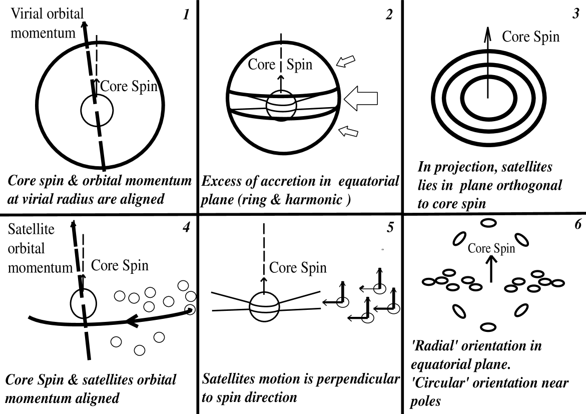
Figure 16: A schematic representation of all estimate of anisotropic accretion considered in this paper. 1): we measured the distribution of the angle between the orbital momentum on the virial sphere and the halo’s spin. The average orbital momentum measured on the virial sphere is mostly aligned with the spin of the halo embedded in the virial sphere (discussed in section 3.2). 2): we compared the accretion in the plane orthogonal to the direction of the halo’s spin with the average accretion on the sphere. On the virial sphere, we detected an excess of ring-like or harmonic accretion in the equatorial plane (discussed in section 3.3 and 3.4). 3): in projection, we used a ‘synthetic’ halo to look at the distribution of satellites detected with ADAPTAHOP and at the orientation of their spin around the direction of the spin. In projection, satellites lie preferentially in the projected equatorial plane (discussed in section 5.1). 4): We measured the angle between the halo’s spin and the orbital momentum of each satellite. The orbital momentum of satellites is preferentially aligned with the spin of their hosting core (discussed in section 4.1). 5): We compared the orientation of each satellite velocity vector (in the core’s rest frame) with the orientation of their own spin. The velocity vector of satellites (in the core’s rest frame) is orthogonal to the direction of their spin (discussed in section 4.2). 6): In the equatorial plane, the projected orientation of satellites is more ’radial’, while near the direction of the spin a ’circular’ configuration of orientation seems to emerge (discussed in section 5.2).

Table 1: Summary of the fitting parameters for the angular correlations

angle	$a_{1}$	$a_{2}$	$a_{3}$	$a_{4}$
$\theta_{\rm\rho L}$	2.351$\pm$0.006	-0.178$\pm$0.002	1.343$\pm$0.002	0.669$\pm$0.000
$\theta_{\rm\rho vrL}$	3.370$\pm$0.099	-0.884$\pm$0.037	1.285$\pm$0.016	0.728$\pm$0.001
$\theta_{\rm cs}$	0.399$\pm$0.003	0.059$\pm$0.008	0.881$\pm$0.005	0.938$\pm$0.000
$\theta_{\rm vs}$	0.295$\pm$0.004	1.544$\pm$0.001	0.804$\pm$0.005	0.914$\pm$0.001
$\theta_{p}$	0.099 $\pm$ 0.003	1.548 $\pm$ 0.003	0.825 $\pm$ 0.013	0.973 $\pm$ 0.000

Here $\theta_{\rm\rho L}$ is the angle between the halo’s spin and the angular momentum measured on the virial sphere; $\theta_{\rm\rho vrL}$ is the angle between the halo’s spin and the accreted angular momentum measured on the virial sphere; $\theta_{\rm cs}$ is the angle between the core’s spin and the satellite orbital momentum; $\theta_{\rm vs}$ is the angle between the satellite velocity in the core ’s rest frame and the satellite’s spin; $\theta_{p}$ is the projected angle between the satellite’s spin and its direction relative to the core s’ position. The fitting model we used is $1+\xi(\theta)=a_{1}/(\sqrt{2\pi}a_{3})\exp\left[-(\theta-a_{2})^{2}/(2a_{3}^{2})\right]+a_{4}$.

Table 2: Summary of other quantities related to anisotropic accretion

$\langle\delta_{m}\rangle(z)$	0.0161($\pm$ 0.0103) z +0.147 ($\pm$ 0.005)
$S_{3}(\delta_{m})$	0.44
$\epsilon(R_{m})$	0.1
${\tilde{a}_{20}}$	-0.65 $\pm$ 0.04
${\tilde{a}_{40}}$	0.12 $\pm$ 0.02
${\tilde{a}_{60}}$	-0.054 $\pm$ 0.015
${\tilde{a}_{80}}$	0.0145 $\pm$ 0.0014

$\langle\delta_{m}\rangle(z)$ is the redshift evolution of the average excess of accretion in the plane orthogonal to the direction of the spin. $S_{3}(\delta_{m})$ is the skewness of the distribution of excess of accretion. $\epsilon(R_{m})$ is the axis ratio $a/b-1$ with $a>b$ of the projected satellite distribution. ${\tilde{a}_{20}}$, ${\tilde{a}_{40}}$, ${\tilde{a}_{60}}$ and ${\tilde{a}_{80}}$ are the normalized harmonic coefficients of the ‘equatorial’ modes.

7.1 Conclusion

Using a set of 500 $\Lambda$CDM simulations, we investigated the properties of the spatial configuration of the cosmic infall of dark matter around galactic $\approx L_{\star}$ haloes. The aim of the present work was to find out if the existence of preferential directions existing on large scales (such as filaments) is reflected in the behaviour of matter accreted by haloes, and the answer is a clear quantitative yes.

Two important assumptions were made in the present paper.We did not consider different class of haloes’ masses (except for Fig. 19), but instead applied normalisations to includes all haloes in our measurements (considering e.g. the statistical average of constrasts). We also did not take in account outflows and focused on accreted quantities.

First we looked at the angular distribution of matter at the interface between the intergalactic medium and the inner regions of the haloes. We measured the accreted mass and the accreted angular momentum at the virial radius, describing these quantities as spherical fields.

• The total (resp. advected) angular momentum measured at the virial radius is strongly aligned with the inner spin of the halo with a proportion of aligned configuration $30\%$ (resp. $50\%$) more frequent than the one expected in an isotropic distribution of accreted angular momentum ($1+\xi_{\mathrm{LS}}(0)\sim 1.5$). This result reflects the importance of accreted angular momentum in the building of the haloes’ inner spin.

• The accretion of mass measured at the virial radius in the ring-like region perpendicular to the direction of the halo’s spin is $\sim 15\%$ larger than the one expected in the case of an isotropic infall of matter.
  We also detected the excess of accretion at the same level in the equatorial plane using a spherical harmonic expansion of the mass density flux.

• In the spin’s frame, the average of the harmonic $a_{\ell 0}$ coefficients does not converge toward zero, indicating that there is a systematic accretion structured in rings parallel to the equatorial plane.

  Using the substructure detection code ADAPTAHOP, we confirmed that the existence of a preferential plane for the infalling mass is reflected in the distribution of satellites around haloes.

• Investigating the degree of alignment between the orbital momentum of satellites and the central spin of the halo, it is shown that the aligned configuration is present in excess of $\sim 12\%$. Satellites tend to revolve in the plane orthogonal to the direction of the halo’s spin. The two methods (using spherical fields and satellites’ detection) yield consistent results and suggest that the image of a spherical infall on haloes should be reconsidered at the quoted level.
  We studied the distribution of the angle between the direction of accretion of satellites and their own spin.

• An orthogonal configuration is $5\%$ more frequent than what would one expect for an isotropic distribution of spin and directions of accretion. Satellites tend to be accreted in the direction orthogonal to their own spin.

  These findings are interpreted as the results of the filamentary flows of structures, where satellites and haloes are accreted along the main direction of filaments with their spins orthogonal to this preferential direction. The flow along filaments also explains why the matter is accreted preferentially in the equatorial plane at the virial radius. The halo points its spin perpendicular to the flow and sees a larger flux in the regions normal to the flow direction, i.e. near the equator. Thus, it appears that the existence of preferential directions on large scales is still relevant on galactic scales and should have consequences for the inner dynamics of the halo.

  We addressed the issue of observing these alignments in projection.

• The distribution of satellites projected onto the sky is flattened, with an axis ratio of $1.1$ at the virial radius.

• It seems that the orientation of satellites around their haloes is not random, even if the two dimensional representation dilutes the effects of alignments. The ‘radial’ orientation, where the satellites main axis is aligned with the line joining the satellite to the halo centre, is $\sim 5\%$ more frequent than the one expected in a completely random distribution of orientation. The ‘circular’ configuration, where the satellites main axis is perpendicular to the line joining the satellite to the halo centre, is also present in excess compared to an random distribution near the pole of the host galaxy.

All corresponding fits are summarized in Table 1 and 2, while Fig. 16 gives a schematic view of the measurements we carried out.

We investigated how the self-consistent dynamical response of the halo would propagate anisotropic infall down to galactic scales. In particular we gave the corresponding polarisation operator in the context of an opened system. We have shown in appendix A that accounting for dark matter infall required the knowledge of the first three moments of the flux densities, $\varpi_{\rho}({{\mbox{\boldmath$\Omega$}}},\tau),\varpi_{\rho{\bf v}}({{\mbox{\boldmath$\Omega$}}},\tau),\varpi_{\rho\sigma_{i}\sigma_{j}}({{\mbox{\boldmath$\Omega$}}},\tau)$.

It is suggested that the existence of a preferential plane of accretion of matter, and thus of angular momentum, should have an influence on warp generation and disk thickening. If the anisotropic properties of infalling matter measured in the outer parts of haloes are conserved in the inner region of galaxies, there may exist a ’typical’ warp amplitude and this anisotropic accretion of matter may explain the properties of warp line of nodes. In the same spirit, the efficiency of the thickening of the disk may be enhanced or reduced by equatorial accretion. Finally, our finding of intrinsic alignments on small scales as well as specific orientations of structures should be relevant for cosmic shear studies on wide and shallow surveys.

7.2 Prospects

The main purpose of our investigation was to provide quantitative measurements of the level of anisotropy involved in the infall on scales $\leq 500$ kpc. The next step should clearly involve working out quantitatively their implications for warp, disk heating etc… as was discussed in section 6.

Our measurements were carried out at $R_{200}$, which on galactic scales is a long way from the inner region of the galaxy. One should clearly propagate the infall (and its anisotropy) towards the centre of the galaxy, and more radial infalling components will play a more important role and should be weighted accordingly. It should also be stressed that we did not take into account the extra polarisation induced by the presence of an embedded disk, which will undoubtedly reinforce the polarisation and the anisotropy of the infall. We also concentrated on mass accretion, as the lowest order moment of the underlying “fluid” dynamics. Clearly higher moments involving the anisotropically accreted momentum, the kinetic energy etc. are dynamically relevant for the evolution of the central object as is discussed in section 6 and in the appendix. The time evolution of the statistics of these flux densities is also essential for the inner dynamic of the halo and should be addressed systematically as well. It will be worthwhile to explore different cosmologies and their implications on small scale dynamics, and on the characteristics of infalling clumps, though we hope that the qualitative results sketched here should persist.

It should be emphasized that some aspects of the present work are exploratory only, in that the resolution achieved ($M_{\mathrm{halo}}>5\cdot 10^{12}M_{\odot}$) is somewhat high for $L_{\star}$ galaxies. In fact, it would be interesting to see if the properties of infall changes for lower mass ($M_{\mathrm{halo}}<5\cdot 10^{10}M_{\odot}$) together with the intrinsic properties of galaxies. In addition a systematic study of biases induced by the estimators of angular correlations should be conducted, e.g. the mass weighted errors we introduced in section 3.2.

Observationaly, the synthetic halo described in section 5.1 could be compared to stacked satellite distributions relying on galactic surveys such as the SDSS. Once the anisotropy has been propagated to the inner regions of the galactic halo following the method sketched in section 6, we should be in a position to compile a synthetic edge-on galactic disk and compare the flaring of the disk with the corresponding predictions. The residual preferred orientation of galactic disks around more massive objects discussed in section 5.2 should be observed on the scales $\leq 500{\rm kpc}$.

Using larger simulations will allow us to combine high resolution with the statistics required to detect the anisotropic accretion of mass and angular momentum. A wide range of halo masses will become accessible and the halo mass dependency of our findings will be constrained without suffering from the lack of statistics. Better angle determinations will naturally follow from a better resolution and will improve the accuracy of our quantitative results. Resimulations (zoom simulations) should give access to a larger range of satellite masses, while we were here mostly sensitive to the biggest substructures. Large infalling objects are likely to feel differently the effects of tidal forces or dynamical friction than smaller satellites. Resimulated haloes allow us to investigate the dependency on the spatial distribution of satellites with their masses corresponding to a given cosmological environment. However using only a few resimulations may not be sufficient to overcome cosmic variance and, given the difficulty to produce a large number of high resolution haloes, such a project remains challenging.

The inclusion of gas physics in these simulations and their impact on the results is the natural following step. For example, gas filaments are known to be narrower than dark matter filaments, thus we expect to see a higher level of anisotropy in the distribution of accreted gas by the haloes. Furthermore, the transmission of angular momentum from one parcel of gas to another (or to the underlying dark matter) may be highly effective and would lead to higher homogeneity of the properties of the accreted angular momentum direction, enhancing the effect of spin alignments. The loss of angular momentum from the gaz to the halo will lead to a modification of our pure dark matter findings. Yet, the inclusion of gas physics in simulations would force us to address issues such as the over-cooling, the requirement to take star formation and related feedback processes into account. It remains that in the longer term, the inclusion of gas physics cannot be avoided and will give new insights into the anisotropic accretion of matter by haloes.

Acknowledgements

We are grateful to J. Devriendt, J. Heyvaerts, A. Kalnajs, D. Pogosyan, E. Scannapieco, F. Stoehr, R. Teyssier, E. Thiébaut, for useful comments and helpful suggestions. DA would like to thank C. Boily for reading early versions of this paper. CP would like to thank F. Bernardeau for stimulating discussions during the premises of this work. We would like to thank D. Munro for freely distributing his Yorick programming language (available at ftp://ftp-icf.llnl.gov:/pub/Yorick), together with its MPI interface, which we used to implement our algorithm in parallel.

Appendix A Linear response of a spherical halo to infalling dark matter fluxes

In the following section, we extend to open spherical stellar systems the formalism developed by Tremaine & Weinberg (1984) and e.g. Murali (1999) by adding a source term to the collisionless Boltzmann equation. For an open system, the dark matter dynamics within the $R_{200}$ sphere is governed by the collisionless Boltzmann equation coupled with the Poisson equation:

$$\frac{{dF}}{{dt}}\equiv\frac{\partial F}{\partial t}+\{F,H\}=s^{e}({\bf r},{\bf v},t),\quad{\rm and}\quad\nabla^{2}\Psi=4\pi G\int{{\mathrm{d}}}^{3}vF({\bf v}).$$ (37)

where $\{\,\,\}$ is the standard Poisson bracket, $F({\bf r},{\bf v},t)$ is the system’s distribution function submitted to $\Psi({\bf r},t)$, the total gravitational potential (self-gravity + external perturbation). The r.h.s. of (37) is non-zero because of infalling fluxes from the environment which require adding a source term, $s^{e}({\bf r},{\bf v},t)$, to the Vlazov equation. We may now discriminate between a stationary part corresponding to the unperturbed state from a weak time-dependent perturbation induced by the environnement. Thus the DF can be written as $F=F_{0}+f$. Provided the mass of the incoming flux of dark matter is small compared to the mass of the halo, we may assume that $f$ is small compared to $F_{0}$. Similarly, the Hamiltonian $H$ of the system can be expanded as $H_{0}+\Delta H$, with $\Delta H=\psi^{e}+\psi$ where $\psi^{e}$ and $\psi$ stand respectively for the external perturbative potential and for the small response in potential of the open system.

A.1 The Boltzmann equation in action-angle

Given the periodicity of the system, the most adequate representation of a spherical halo corresponds to action-angle variables (Goldstein (1950)). The linearized Boltzmann equation in such a representation is:

$$\frac{\partial f_{\bf k}({\bf I},t)}{\partial t}+\imath{\bf k}\cdot{{{\mbox{\boldmath$\omega$}}}}f_{\bf k}({\bf I},t)=\imath{\bf k}\cdot\frac{{{\mathrm{d}}}{}F_{0}}{{{\mathrm{d}}}{\bf I}}\Delta H_{\bf k}({\bf I},t)+s^{e}_{\bf k}({\bf I},t).$$ (38)

The new variables are the actions ${\bf I}$ and the angles ${\bf w}$ together with the angular rates ${{\mbox{\boldmath$\omega$}}}\equiv{{\mathrm{d}}}{\bf w}/{{\mathrm{d}}}t$. In equation 38 we have Fourier expanded the linearized equation 37 over the periodic angles:

$$X({\bf r},{\bf v},t)=\sum_{{\bf k}}X_{\bf k}({\bf I},t)\exp{(\imath{\bf k}\cdot{\bf w})},\quad{\rm with}\quad X_{{\bf k}}({\bf I},t)=\frac{1}{(2\pi)^{3}}\int{{\mathrm{d}}}^{3}{{\bf w}}\exp(-\imath{\bf k}\cdot{\bf w})X({\bf r},{\bf v},t),$$ (39)

where $X$ is any function of $({\bf r},{\bf v},t)$ with ${\bf k}$ being the Fourier triple index corresponding to the three degrees of freedom on the sphere. The equilibrium state $F_{0}$ does not depend on time nor angles since it is assumed to be stationary. Then the solution to (38) can be written as:

$$f_{\bf k}({\bf I},t)=\int_{-\infty}^{t}{{\mathrm{d}}}\tau\exp(\imath{\bf k}\cdot{\bf\omega}(\tau-t))\left[\imath{\bf k}\cdot\frac{{{\mathrm{d}}}F_{0}}{{{\mathrm{d}}}{\bf I}}\left[\psi_{\bf k}({\bf I},\tau)+\psi^{e}_{\bf k}({\bf I},\tau)\right]+s^{e}_{\bf k}({\bf I},\tau)\,\right],$$ (40)

where we have written $\Delta H_{\bf k}({\bf I},\tau)=\psi_{\bf k}({\bf I},\tau)+\psi^{e}_{\bf k}({\bf I},\tau)$. We can integrate (40) over velocities and sum over ${\bf k}$ to recover the density perturbation:

$$\rho({\bf r},t)=\sum_{{\bf k}}\int_{-\infty}^{t}{{\mathrm{d}}}\tau\int{{\mathrm{d}}}^{3}{\bf v}\left(\exp(\imath{\bf k}\cdot{{{\mbox{\boldmath$\omega$}}}}(\tau-t)+\imath{\bf k}\cdot{\bf w})\left[\imath{\bf k}\cdot\frac{{{\mathrm{d}}}F_{0}}{{{\mathrm{d}}}{\bf I}}\left[\psi_{\bf k}({\bf I},\tau)+\psi^{e}_{\bf k}({\bf I},\tau)\right]+s^{e}_{\bf k}({\bf I},\tau)\,\right]\right).$$ (41)

Let us expand the potential and the density over a bi-orthogonal complete basis function $\{\psi^{[{\mathbf{n}}]},\rho^{[{\mathbf{n}}]}\}$such that

$$\psi({\bf r},t)=\sum_{{\mathbf{n}}}a_{{\mathbf{n}}}(t)\psi^{[{\mathbf{n}}]}({\bf r})\,;\quad\rho({\bf r},t)=\sum_{{\mathbf{n}}}a_{{\mathbf{n}}}(t)\rho^{[{\mathbf{n}}]}({\bf r})\,;\quad\nabla^{2}\psi^{[{\mathbf{n}}]}=4\pi G\rho^{[{\mathbf{n}}]}\,;\quad\int{{\mathrm{d}}}^{3}{\bf r}\psi^{[{\mathbf{n}}]*}({\bf r})\rho^{[{\mathbf{p}}]}({\bf r})=\delta^{n}_{p}.$$ (42)

The external potential can be expanded along the same basis as:

$$\quad\psi^{e}({\bf r},t)=\sum_{{\mathbf{n}}}b_{{\mathbf{n}}}(t)\psi^{[{\mathbf{n}}]}({\bf r}).$$ (43)

Note that in Eq. (42) the expansion runs over a triple index ${\mathbf{n}}\equiv(n,\ell,m)$ corresponding to the radial, azimuthal and alt-azimuthal degrees of freedom, while in Eq. (42) the three coefficients are not independent since the radial variation of the external potential is fixed by its boundary value on the sphere $R_{200}$. Making use of the biorthogonality, multiplying (41) by $\psi^{[{\mathbf{p}}]*}({\bf r})$ for some given ${\mathbf{p}}$ and integrating over ${\bf r}$ yields:

$$a_{{\mathbf{p}}}(t)=\sum_{{\bf k}}\int_{-\infty}^{t}{{\mathrm{d}}}\tau\int\int{{\mathrm{d}}}^{3}{\bf v}{{\mathrm{d}}}^{3}{\bf r}\exp(\imath{\bf k}\cdot{{{\mbox{\boldmath$\omega$}}}}(\tau-t)+\imath{\bf k}\cdot{\bf w})\psi^{[{\mathbf{p}}]*}({\bf r})\left[\sum_{{\mathbf{n}}}\imath{\bf k}\cdot\frac{{{\mathrm{d}}}F_{0}}{{{\mathrm{d}}}{\bf I}}\left[a_{{\mathbf{n}}}(\tau)+b_{{\mathbf{n}}}(\tau)\right]\psi^{[{\mathbf{n}}]}_{\bf k}({\bf I})+{s}^{e}_{\bf k}({\bf I},\tau)\,\right]$$ (44)

A.2 Self-consistency of the response

We may now swap from position-velocity to angle-action variables since ${{\mathrm{d}}}^{3}{\bf v}{{\mathrm{d}}}^{3}{\bf r}={{\mathrm{d}}}^{3}{\bf w}{{\mathrm{d}}}^{3}{\bf I}$. In (44) only $\psi^{[{\mathbf{p}}]}({\bf r})$ depends on ${\bf w}$ so we may carry the ${\bf w}$ integration over $\psi^{[{\mathbf{p}}]*}$, yielding $\psi^{[{\mathbf{p}}]*}_{\bf k}({\bf I})$ which leads to

$$a_{{\mathbf{p}}}(t)=\sum_{{\bf k}}\int_{-\infty}^{t}{{\mathrm{d}}}\tau\int{{\mathrm{d}}}^{3}{\bf I}\exp(\imath{\bf k}\cdot{{{\mbox{\boldmath$\omega$}}}}(\tau-t))\left[\sum_{{\mathbf{n}}}\imath{\bf k}\cdot\frac{{{\mathrm{d}}}F_{0}}{{{\mathrm{d}}}{\bf I}}\left[a_{{\mathbf{n}}}(\tau)+b_{{\mathbf{n}}}(\tau)\right]\psi^{[{\mathbf{p}}]*}_{\bf k}({\bf I})\psi^{[{\mathbf{n}}]}_{\bf k}({\bf I})+{s}^{e}_{\bf k}({\bf I},\tau)\,\psi^{[{\mathbf{p}}]*}_{\bf k}({\bf I})\right]$$ (45)

Note that the last term of Eq. (45) corresponds to the modulated potential along the unperturbed trajectories weighted by the number of entering particles with $({\mathbf{v}},{\mbox{\boldmath$\Omega$}})$ at time $\tau$. This is expected since it just reflects the fact that could have linearly summed over all incoming individual particles (since the interaction between particles in a collisionless fluid is purely gravitationnal). In this sense, this terms corresponds to a ray tracing problem in a variable index medium. Note also that Eq. (45) does not account for dynamical friction since we integrate over the unperturbed trajectories. At this point, we expand the source term over a complete basis; this basis should also describe (known) velocity space variations. We assume that such a basis $\phi^{[{\mathbf{n}}]}({\bf r},{\bf v})$ exists. We write:

$$s^{e}({\bf r},{\bf v},t)=\sum_{{\mathbf{n}}}c_{{\mathbf{n}}}(t)\phi^{[{\mathbf{n}}]}({\bf r},{\bf v})\,\,\,{\rm so}\,\,{s}^{e}_{\bf k}({\bf I},\tau)\,=\sum_{{\mathbf{n}}}c_{{\mathbf{n}}}(\tau){\sigma}^{[{\mathbf{n}}]e}_{\bf k}({\bf I})\,\,{\rm where}\,\,{\sigma}^{[{\mathbf{n}}]e}_{\bf k}({\bf I})\equiv\frac{1}{(2\pi)^{3}}\int{{\mathrm{d}}}^{3}{{\bf w}}\exp(-\imath{\bf k}\cdot{\bf w})\phi^{[{\mathbf{n}}]}({\bf r},{\bf v}).$$ (46)

Calling ${\bf a}(\tau)=[a_{{\mathbf{1}}}(\tau),\cdots,a_{{\mathbf{n}}}(\tau)]$, ${\bf b}(\tau)=[b_{{\mathbf{1}}}(\tau),\cdots,b_{{\mathbf{n}}}(\tau)]$, ${\bf c}(\tau)=[c_{{\mathbf{1}}}(\tau),\cdots,{c}_{{\mathbf{n}}}(\tau)]$, and $\Theta(\tau)$ the Heaviside function, we define two tensors:

$${K}_{{\mathbf{p}}{\mathbf{n}}}(\tau)=(1-\Theta(\tau))\cdot\sum_{{\bf k}}\int{{\mathrm{d}}}^{3}{\bf I}\exp(\imath{\bf k}\cdot{{{\mbox{\boldmath$\omega$}}}}\tau)\imath{\bf k}\cdot\frac{{{\mathrm{d}}}F_{0}}{{{\mathrm{d}}}{\bf I}}\psi^{[{\mathbf{p}}]*}_{\bf k}({\bf I})\psi^{[{\mathbf{n}}]}_{\bf k}({\bf I}),$$ (47)

which depends only on the halo equilibrium state via $F_{0}$ and

$${H}_{{\mathbf{p}}{\mathbf{n}}}(\tau)=(1-\Theta(\tau))\cdot\sum_{{\bf k}}\int{{\mathrm{d}}}^{3}{\bf I}\exp(\imath{\bf k}\cdot{{{\mbox{\boldmath$\omega$}}}}\tau){\sigma}^{[{\mathbf{n}}]e}_{\bf k}({\bf I})\,\psi^{[{\mathbf{p}}]*}_{\bf k}({\bf I}),$$ (48)

which depends only on the expansion basis, equation (45) becomes:

$${\bf a}(t)=\int_{-\infty}^{\infty}{{\mathrm{d}}}\tau\left\{{\bf K}(\tau-t)\cdot\left[{\bf a}(\tau)+{\bf b}(\tau)\right]+{\bf H}(\tau-t)\cdot{\bf c}(\tau)\right\}.$$ (49)

We now perform a Fourier transform with respect to time, hence convolutions become multiplications and we get:

$${\bf\hat{a}}(p)=({\bf I}-{\bf\hat{K}}(p))^{-1}\cdot\left[{\bf\hat{K}}(p)\cdot{\bf\hat{b}}(p)+{\bf\hat{H}}(p)\cdot{\bf\hat{c}}(p)\right],$$ (50)

where $p$ stands for the frequency conjugate to time. The computation of the variance-covariance matrix is straightforward:

$$\langle{{\mathbf{\hat{a}}}}\cdot{{\mathbf{\hat{a}}}}^{*{{}^{\top}}}\rangle=\langle({\bf I}-{\bf\hat{K}})^{-1}\cdot\left[{\bf\hat{K}}\cdot{\bf\hat{b}}+{\bf\hat{H}}\cdot{\bf\hat{c}}\right]\cdot\left[{\bf\hat{K}}\cdot{\bf\hat{b}}+{\bf\hat{H}}\cdot{\bf\hat{c}}\right]^{{{}^{\top}}*}\cdot({\bf I}-{\bf\hat{K}})^{-1*{{}^{\top}}}\rangle\,,$$ (51)

where ${\bf I}$ the identity matrix. Note that $\langle{{\mathbf{\hat{a}}}}\cdot{{\mathbf{\hat{a}}}}^{*{{}^{\top}}}\rangle$ involves autocorrelation like $\langle{{\mathbf{\hat{b}}}}\cdot{{\mathbf{\hat{b}}}}^{*{{}^{\top}}}\rangle$ and $\langle{{\mathbf{\hat{c}}}}\cdot{{\mathbf{\hat{c}}}}^{*{{}^{\top}}}\rangle$ but also cross correlation terms such as $\langle{{\mathbf{\hat{b}}}}\cdot{{\mathbf{\hat{c}}}}^{*{{}^{\top}}}\rangle$. In other words, recalling that ${\mathbf{b}}$ and ${\mathbf{c}}$ stand respectively for the expansion coeficients of the external potential, Eq. (43), and the parametrized velocity distribution, Eq. (46), their cross-correlation will in fine modify the correlation of the response of the inner halo. Two-points statistics are sufficient to caracterize stationnary perturbations and therefore the induced response. Nevertheless, higher statistics of the response can be easily expressed in terms of higher order correlations of the pertubation if needed. For example, it can be shown that the three-point correlation function of the response’s coefficients can be written as function of the two- and three-points correlation of the perturbations’ coefficients. There are yet quite a few caveats involved; for instance, it is not completely clear today that we have a good understanding of what the unperturbed distribution function of a halo+disk should be.

A.3 The source term

A possible choice for the source term consistent with the first two velocity moments of the entering matter, involves constructing $s^{e}({\bf r},{\bf v},t)$ in the following manner:

$$s^{e}({\bf r},{\bf v},t) = \sum_{\bf m}Y_{{\mathbf{m}}}({{\mbox{\boldmath$\Omega$}}})\frac{\delta_{\rm D}(r-R_{200})\,{\hat{\varpi}}_{\rho,{\mathbf{m}}}(t)(2\pi)^{-3/2}}{{\rm det}|{{\hat{\varpi}}_{\rho\sigma_{i}\sigma_{j},{\mathbf{m}}}(t)}/{{\hat{\varpi}}_{\rho,{\mathbf{m}}}}(t)|\,\,}\exp\left[-\frac{1}{2}\left({\bf v}-\frac{{\hat{\varpi}}_{\rho{\bf v},{\mathbf{m}}}(t)}{{\hat{\varpi}}_{\rho,{\mathbf{m}}}(t)}\right)^{{{}^{\top}}}\left(\frac{{\hat{\mbox{\boldmath$\varpi$}}}_{\rho\sigma_{i}\sigma_{j},{\mathbf{m}}}(t)}{{\hat{\varpi}}_{\rho,{\mathbf{m}}}(t)}\right)^{-1}\left({\bf v}-\frac{{\hat{\varpi}}_{\rho{\bf v},{\mathbf{m}}}(t)}{{\hat{\varpi}}_{\rho,{\mathbf{m}}}(t)}\right)\right]$$ (52)

$$\equiv \sum_{\bf m}Y_{{\mathbf{m}}}({{\mbox{\boldmath$\Omega$}}})\delta_{\rm D}(r-R_{200}){\cal C}_{{\mathbf{m}}}({\bf v},t)\,,$$

where ${\mathbf{m}}$ stands for the two harmonic number, $(\ell,m)$ and $Y_{{\mathbf{m}}}({{\mbox{\boldmath$\Omega$}}})\equiv Y_{\ell}^{m}({{\mbox{\boldmath$\Omega$}}})$. Here the Dirac function $\delta_{\rm D}(r-R_{200})$ is introduced since we measure the source terms at the virial radius. The global form is Gaussian and is constructed using ${\hat{\varpi}}_{\rho,{\mathbf{m}}}$, ${\hat{\varpi}}_{\rho{\bf v},{\mathbf{m}}}$, ${\hat{\varpi}}_{\rho\sigma_{i}\sigma_{j},{\mathbf{m}}}$, the harmonic components of respectively the mass flux density field, velocity flux density vector field and the specific kinetic energy flux density tensor field measured on the $R_{200}$ sphere. When taking the successive moment of this flux distribution over velocity, we get:

$$\int{{\mathrm{d}}}{}^{3}{\mathbf{v}}s^{e}({{\bf r}},{\bf v})={\varpi}_{\rho}({\bf r})\,,\quad\int{{\mathrm{d}}}{}^{3}{\mathbf{v}}{\bf v}s^{e}({{\bf r}},{\bf v})={\varpi}_{\rho{\mathbf{v}}}({\bf r})\,,$$ (53)

while

$$\quad\int{{\mathrm{d}}}{}^{3}{\mathbf{v}}{(v_{i}-\frac{{\varpi}_{\rho{\bf v},i}}{{\varpi}_{\rho}})}\,{(v_{j}-\frac{{\varpi}_{\rho{\bf v},j}}{{\varpi}_{\rho}})}s^{e}({\bf r},{{\bf v}})={\varpi}_{\rho\sigma_{i}\sigma_{j}}({\bf r})+\left(\sum_{\bf m}Y_{{\mathbf{m}}}({{\mbox{\boldmath$\Omega$}}})\delta(r-R_{200})\frac{{\hat{\varpi}}_{\rho{\bf v},{\mathbf{m}}}(t)^{2}}{{\hat{\varpi}}_{\rho,{\mathbf{m}}}(t)}-\frac{{\varpi}_{\rho{\mathbf{v}}}({\bf r})^{2}}{{\varpi}_{\rho}({\bf r})}\right)\approx{\varpi}_{\rho\sigma_{i}\sigma_{j}}({\bf r}),$$ (54)

so that the Ansatz, Eq. (52), satisfy the first two moments, and approximatively the third moment of the fluid equations. Let us now expand ${\cal C}_{{\mathbf{m}}}({\bf v},t)$ over a linear complete basis, say b-splines covering the radial velocity component and spherical harmonics for the angle distribution of the velocity vector:

$${\cal C}_{{\mathbf{m}}}({\bf v},t)=\sum_{\alpha}C_{{\mathbf{m}},\alpha}(t)b_{\alpha}({\bf v}).$$ (55)

The particular choice of Eq. (52) has led to the parametrisation:

$$c_{{\mathbf{n}}}(t)={C}_{{\mathbf{m}},\alpha}(t)\quad{\rm and}\quad\phi^{[{\mathbf{n}}]}({\bf r},{\bf v})=b_{\alpha}({\bf v})\,Y_{{\mathbf{m}}}({{\mbox{\boldmath$\Omega$}}})\delta_{\rm D}(r-R_{200})\,,$$ (56)

while Eq. (46) becomes

$${\sigma}^{[{\mathbf{n}}]e}_{\bf k}({\bf I})=\frac{1}{(2\pi)^{3}}\int{{\mathrm{d}}}^{3}{{\bf w}}\exp\left(-\imath{\bf k}\cdot{\bf w}\right)Y_{{\mathbf{m}}}[{{\mbox{\boldmath$\Omega$}}}({\bf I},{\bf w})]b_{\alpha}({\bf v}[{\bf I},{\bf w}])\delta_{\rm D}(r({\bf I},{\bf w})-R_{200})\,.$$ (57)

Note that we can make use of the $\delta_{\rm D}$ function occurring in Eq. (57) since $w_{r}\equiv{\tilde{w}}_{r}(r,{\bf I})$. Therefore Eq. (57) reads:

$${\sigma}^{[{\mathbf{n}}]e}_{\bf k}({\bf I}) = \int\frac{{{\mathrm{d}}}^{2}{{\bf w}}}{(2\pi)^{3}}\int{{\mathrm{d}}}w_{r}\exp\left(-\imath{\bf k}\cdot{\bf w}\right)Y_{{\mathbf{m}}}[{{\mbox{\boldmath$\Omega$}}}({\bf I},{\bf w})]b_{\alpha}({\bf v}[{\bf I},{\bf w}])\frac{1}{|\partial{\tilde{w}}_{r}/\partial r|^{-1}}\delta_{\rm D}(w_{r}-{\tilde{w}}_{r}[R_{200},{\bf I}])\,,$$ (58)

$$= \int\frac{{{\mathrm{d}}}^{2}{{\bf w}}}{(2\pi)^{3}}\exp\left(-\imath{\bf k}\cdot{\bf w}\right)Y_{{\mathbf{m}}}[{{\mbox{\boldmath$\Omega$}}}({\bf I},{\bf w},{\tilde{w}}_{r}[R_{200},{\bf I}])]b_{\alpha}({\bf v}[{\bf I},{\bf w},{\tilde{w}}_{r}(R_{200},{\bf I})])\frac{\omega_{r}({\bf I})}{|{\dot{r}}(R_{200},{\bf I})|}\exp\left(-\imath k_{r}\cdot{\tilde{w}}_{r}[R_{200},{\bf I}]\right)$$

In Eq. (58) we sum over all intersections of the orbit ${\bf I}$ with the $R_{200}$ sphere, at the radial phase corresponding to that intersection (with a weight corresponding to $\omega_{r}/|{\dot{r}}|$).

Given Eq. (42), Eq. (52), together with Eq. (58), Eq. (49) can be recast formally as

$$\rho({\mathbf{r}},t)={\mathbf{R}}\{F_{0},t,\tau,{{\mbox{\boldmath$\Omega$}}}\}\left[\psi_{e}({{\mbox{\boldmath$\Omega$}}},\tau),\varpi_{\rho}({{\mbox{\boldmath$\Omega$}}},\tau),\varpi_{\rho{\bf v}}({{\mbox{\boldmath$\Omega$}}},\tau),\varpi_{\rho\sigma_{i}\sigma_{j}}({{\mbox{\boldmath$\Omega$}}},\tau)\right]$$ (59)

which corresponds to the form given in the main text in Equation 31. It should be emphasized once again that the splitting of the gravitationnal field into two components, one outside of $R_{200}$, and one inside, via point particles obeying the distribution $s_{e}({\mathbf{r}},{\mathbf{v}},t)$ is completely arbitrary from the point of view of the dynamics. In fact, one should account that $\psi_{e}({\mbox{\boldmath$\Omega$}},t)$ should be switched on long before any particles enter $R_{200}$ since no particle is created at the boundary. This last constraint is clearly satisfied by our simulations.

Appendix B ADAPTAHOP: a substructure finder based on saddle point handling

Dark matter haloes can contain a hierarchy of subhaloes, which can be viewed as a tree of structures and sub-structures. Given a mass resolution (a finite number of particles such as in our $N$-body simulations), there is a limit to this hierarchy, which can be formalised as an ensemble of leaves in a tree. The goal here is to draw this tree by applying the simplest principles of Morse theory (e.g. Jost (2002)). Morse theory basically involves relating the topology of an excursion, e.g., the regions of space with density above a given threshold, $\rho>\rho_{\rm t}$, to the set of critical points it contains, $\{{\bf x},\nabla\rho({\bf x})=0\}$, and to the field lines connecting these points together, i.e. the curves obtained by following the gradient of the density field. In that approach, the smallest substructures, which are the leaves of the tree, can be identified as peak patches, i.e. ensembles of field lines converging to the same local maximum. The connectivity between substructures is ruled by the saddle points, which are local maxima in the surfaces defining the contours of the peak patches: from the knowledge of these saddle points and the local maxima they connect, it is possible to extract the full tree of structures (haloes) and sub-structures (subhaloes) in four steps:

1. In order to eliminate, at least partly, the effects of Poisson noise and to have an estimate of the local density as close as possible to a Morse function, while conserving as much as possible details of the distribution, we perform adaptive smoothing of this distribution with standard SPH technique (Smooth Particle Hydrodynamics, e.g. Monaghan (1992)). This smoothing assumes that each particle is a smooth spherical cloud of given radius $R$, e.g. a spline $S(r)$. For each particle, the list of its $N_{\rm SPH}$ closest neighbors is found, typically $N_{\rm SPH}$ of a few tens (here we take $N_{\rm SPH}=64$). The distance from the furthest neighbor fixes $R$, while the SPH density at the particle of interest is estimated by a summation over its neighbors with weight $S(r)$. To find rapidly the closest neighbors of each particle, we use a standard Oct-tree algorithm, which decomposes hierarchically space in subcells untill they contain zero or one particle.

2. The leaves of the tree of structures and substructures are identified while associating each particle to the peak patch it belongs to. This is performed by a simple walk from particle to particle, while following the gradient until convergence: at each step of the walk, the SPH density of the particle is compared to its $N_{\rm HOP}$ closest neighbors (which were stored during the SPH smoothing step), the particle for the next step of the walk being the one with the largest SPH density. We take $N_{\rm HOP}=16$, as advocated by Eisenstein & Hut (1998).

3. For each leave of the tree, the connections with the other leaves are created by searching the saddle points on the intersecting surfaces ${\cal S}_{ij}$ between peak patches $i$ and $j$. Each surface ${\cal S}_{ij}$ is made of particles belonging to one of the peak patches and having at least one of their closest neighbors among $N_{\rm HOP}$ in the other peak patch, and vice versa. If the set ${\cal S}_{ij}$ contains only particles belonging to $i$ or only particles belonging to $j$, the connection between $i$ and $j$ is considered as non significant (because non symmetric) and eliminated, ${\cal S}_{ij}=\hbox{}$. Saddle points are local maxima in ${\cal S}_{ij}$. To establish the connectivity as a function of a density threshold, only the highest saddle point matters, when there are several. The search for this saddle point involves finding the maximum of the SPH density among particles belonging to $S_{ij}$. We proceed as follows to estimate accurately the SPH density in $S_{ij}$. For each particle $A$ in $S_{ij}$, say belonging to peak patch $i$ and with density $\rho_{A}$, we consider the list of its closest neigbors among $N_{\rm HOP}$ belonging to peak patch $j$, with density $\rho_{k}$, $k=1,\cdots,N_{j}\leq N_{\rm HOP}$. The density associated to this particle in ${\cal S}_{ij}$ is then given by $\rho=\min(\rho_{A},\rho_{k})$. By applying this procedure, we locate accurately $S_{ij}$ and avoid slight overestimation of the SPH density at the saddle point.

4. It is possible to build the tree of structures and sub-structures, when the list of neighboring leaves to which a given leave is connected is given, as well as the corresponding saddle points. This is performed recursively by increasing progressively a threshold parameter, $\rho_{\rm t}$, from an initial value, $\rho_{\rm TH}$, corresponding to the typical overdensity used to select galaxy haloes, here called structures. A typical choice for $\rho_{\rm TH}$ is $\rho_{\rm TH}=81$, which corresponds approximately to friend-of-friend haloes selected with a linking paremeter $b=0.2$ (e.g., Eisenstein & Hut (1998)). Suppose we are at step $n$ of the process and let us compute step $n+1$. At this point, we are sitting on a branch of the tree –a structure or a sub-structure– and we aim to draw the details of this branch. This (sub-) structure contains a number of peak patches connected by saddle points of densities $\rho_{\rm s}$. For the considered value of $\rho_{\rm t}$, the connections inside that (sub-) structure are examined and destroyed when $\rho_{\rm s}<\rho_{\rm t}$. The (sub-) structure is then broken into as many components as necessary. During the process, the particles above $\rho_{\rm t}$ belonging to each sub-component are tagged, which allows us to determine at any time various properties of a given (sub-) structure, namely the number of particles it contains, its mass, its average and maximum SPH density, for possible application to various morphological criterions of selection. One such criterion is Poisson noise. In order to asses if a given sub-structure containing $N$ particles should be considered as statistically significant compared to Poisson noise, its average density must be sufficiently significant compared to $\rho_{\rm t}$:

   $$\langle\rho\rangle_{\rm sub-structure}>\rho_{\rm t}\left[1+\frac{f_{\rm Poisson}}{\sqrt{N}}\right],$$ (60)

   where $f_{\rm Poisson}$ is a “$f_{\rm Poisson}\sigma$” detection parameter, typically a few unities. A good choice is $f_{\rm Poisson}=4$. If the sub-structure is below this threshold, it disappears, i.e. it is not considered in next step of the recursion. At the end of the selection, two situations are possible: (i) two sub-structures or more are detected and new nodes are created in the tree (ii) the (sub)-structure was not broken into multiple components and nothing happens at this step. The process is then repeated on the new sub-structures by increasing locally the threshold $\rho_{\rm t}$:

   $$\rho_{\rm t}\rightarrow\rho_{\rm t}\times\left[1+\frac{f_{\rm Poisson}}{\sqrt{N}}\right],$$ (61)

   until there is only one peak patch in the (sub-)structure. Note that the Poisson noise selection, eq. (60) is not applied to the haloes, when $\rho_{\rm t}=\rho_{\rm TH}$.

At the end of the process, one obtains a tree of structures and sub-structures, where each node of the tree corresponding to a (sub-)structure, with its position, its number of particles, is mean square radius, its average and maximum SPH density, and the density $\rho_{\rm s}$ of the highest saddle point which connects it to another substructure. In addition, a flag is given to each particle. This flag is a pointer to the node the closest possible to a leave (if not a leave), which allows one to find recursively the list of particles belonging to any (sub-)structure and thus perform some more ellaborate post-treatement, such as some relying on dynamical prescriptions (boundness). The difficulty in that case is to estimate accuratly the gravitational potential. Its computation can be rather costly, since “pealing” the (sub-)haloes requires iterating several forward and backward walks in the tree of structures and sub-structures with corresponding calculations of the gravitational potential. Our prescription is therefore at the present time purely morphological and does not involve the estimate of the gravitational potential. The current implementation is rather fast, most of the CPU time being taken by the SPH smoothing, e.g. 1-3 hours on 16 millions particles on current fast scalar processors.

Our algorithm is called ADAPTAHOP since we aim at improving HOP (Eisenstein & Hut (1998)): the first two step above are exactly the same as in HOP, but the last two are different. Indeed, in HOP, the idea is to combine informations on the saddle point densities, $\rho_{\rm s}$, on the local maxima, $\rho_{\rm max}$, inside a connected set of peak patches to decide whether it has to be broken into multiple disjoint haloes. The aim of HOP is indeed to improve standard friend-of-friend methods in order to obtain more compact and spherical haloes. The goal of ADAPTAHOP is quite different since it focuses on sub-structure detection.

In spirit, ADAPTAHOP is in fact very similar to the substructure finder of Springel (1999): SUBFIND (see also Springel et al. (2001)). Of course, there is a major difference, since SUBFIND has in addition a sophisticated dynamical prescription involving exact calculation of the gravitationnal potential. Springel uses also a slightly more elegant method to construct the tree of structures and substructures prior to dynamical post-treatment. After step one above, the idea is to rank the particles by decreasing density and treat them in this order. Investigating the distribution of particules is such a way is equivalent to examining isocontours of decreasing density. It uses (as in ADAPTAHOP) the closests neighbors of a particle to decide if the particle examined during the process (i) creates a new (sub-)structure since it is isolated (ii) belongs to an existing substructure or (iii) connects two substructures, which makes the construction of the tree of structures and substructures much simpler than in ADAPTAHOP and more accurate, since there no need for using the threshold parameter $\rho_{\rm t}$. In SUBFIND, no treatment is made to account for the local Poisson noise: it is not necessary because of the dynamical post-processing, which destroys unbounded structures.

It is important to note that since ADAPTAHOP has no dynamical post-treatment, it gives slightly different results compared to SUBFIND in its present form. In particular, for a given sufficiently massive dark matter halo , SUBFIND (Springel et al. (2001)) describes it in terms of a large, smooth central component, and a bunch of much less massive sub-haloes. In ADAPTAHOP, the result is quite similar, except that the central component is much less spatially extended (it is extended up to the isocontour level corresponding to the saddle point connecting it to a sub-halo), and it is therefore less massive.

Fig. 17 illustrates how well ADAPTAHOP performs in one of the simulations we realized for this work, for the most massive halo detected in this realization.

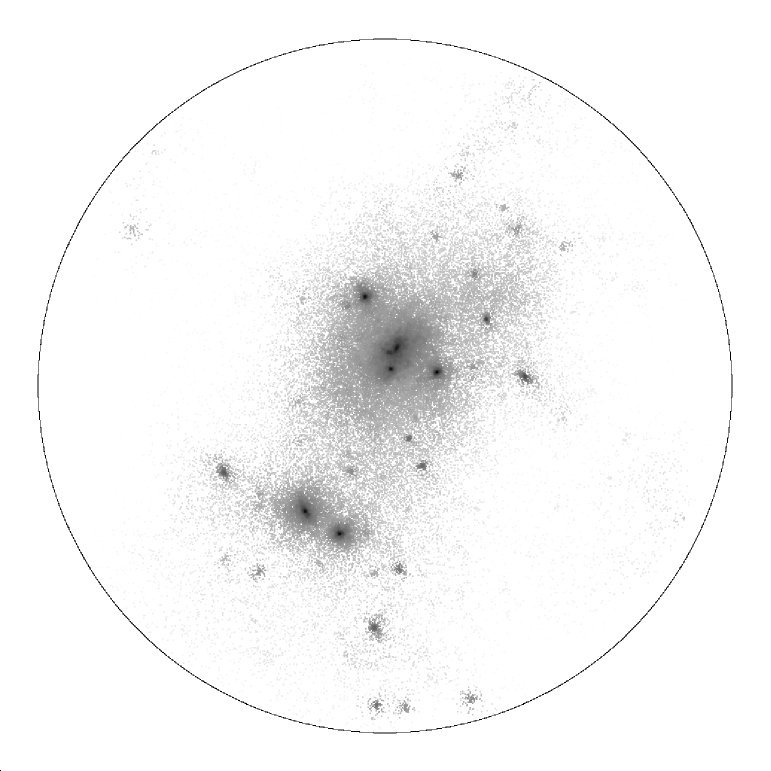
Figure 17: Illustration of the output of ADAPTAHOP for one of the simulations of this work. A sphere of radius 5 Mpc centered on the most massive halo is represented. In the upper pannel, the dark matter density is shown using a logarithmic scale. Darker regions correspond to higher density contrasts. The lower pannel displays the detected subhaloes (i.e. the most elementary structures corresponding to the peak patches or the leaves of the tree). The size of the circle scales with $M^{1/3}$, where $M$ is the mass of the subhalo. Most of the subhaloes seen on the figure belong to the most massive halo. Clearly, ADAPTAHOP is rather successfull at detecting all the significant substructures.

Appendix C Statistics on the sphere

When dealing with spherical fields, there are different ways to characterize their angular structure. In the present paper, we essentially deal with centered statistics, i.e. we describe the angular structuration of scalar or vector fields relative to a specific direction, defined by the halo or satellite’s spin $\bf S$. Let us first formally introduce filtering on the sphere, statistical and angular averages, and present one-point statistics (probability distribution functions) while postponing two-point statistics (correlation functions, or excess probability of joint events) to Aubert & Pichon (2004).

C.1 One point statistics

For any field, $x$, on the sphere, let us introduce the smoothed field, $(x)_{\alpha}$ (filtered on scale $\alpha$) , as

$$(x)_{\alpha}({\mbox{\boldmath$\Omega$}}) \equiv \frac{1}{\int\Theta_{\alpha}({\mbox{\boldmath$\Omega$}}^{\prime})\mathrm{d}{\mbox{\boldmath$\Omega$}}^{\prime}}\int\Theta_{\alpha}({\mbox{\boldmath$\Omega$}}^{\prime}-{\mbox{\boldmath$\Omega$}})x({\mbox{\boldmath$\Omega$}}^{\prime})\mathrm{d}{\mbox{\boldmath$\Omega$}}^{\prime}$$ (62)

$$\equiv \int w_{\alpha}({\mbox{\boldmath$\Omega$}}-{\mbox{\boldmath$\Omega$}}^{\prime})x({\mbox{\boldmath$\Omega$}}^{\prime})\mathrm{d}{\mbox{\boldmath$\Omega$}}^{\prime},$$ (63)

where $\Theta_{\alpha}$stands for the top hat function,

$$\Theta_{\alpha}({\mbox{\boldmath$\Omega$}})=1\quad\textrm{if \quad}|\vartheta|\leqslant\alpha,$$ (64)

and $w_{\alpha}$ is defined by 68 the standard top hat filter on the sphere.

Consider now the centered top-hat-filtered (on scale $\alpha$) field, $[x]_{\alpha}$, defined by

$$[x]_{\alpha} \equiv (x)_{\alpha}(\frac{\pi}{2}),$$ (65)

$$\equiv \frac{1}{\int\Theta_{\alpha}({\mbox{\boldmath$\Omega$}}^{\prime})\mathrm{d}{\mbox{\boldmath$\Omega$}}^{\prime}}\int\Theta_{\alpha}({\vartheta}^{\prime}-\pi/2)x({\mbox{\boldmath$\Omega$}}^{\prime})\mathrm{d}{\mbox{\boldmath$\Omega$}}^{\prime},$$ (66)

$$\equiv \int W_{\alpha}({\mbox{\boldmath$\Omega$}}^{\prime})x({\mbox{\boldmath$\Omega$}}^{\prime})\mathrm{d}{\mbox{\boldmath$\Omega$}}^{\prime}.$$ (67)

Note that Eq. (67) defines $W_{\alpha}$. Our filtering is now centred, in that the average is carried on a window which is centred at the equatorial plane (since we are in this paper interested in the polarisation of accretion processes with respect to that plane). Let us also introduce the average of $x$ on the sphere, as

$${\bar{x}}\equiv(x)_{\pi/2}=\frac{1}{\int\mathrm{d}{\mbox{\boldmath$\Omega$}}}\int x({\mbox{\boldmath$\Omega$}})\mathrm{d}{\mbox{\boldmath$\Omega$}},$$ (68)

We may also for a given $x$ define its contrast as

$$\delta_{x}\equiv\frac{x}{\bar{x}}-1.$$ (69)

Note that, in contrast to standard cosmology, we expect that $\bar{x}\neq\langle x\rangle$, (i.e. no ergodicity) since the angular average over one virial sphere is not representative of the whole cosmological set, and since $\langle x\rangle$ depends on $\vartheta$ whereas $\bar{x}$ doesn’t. As a consequence,

$$\langle\delta_{x}\rangle=\langle\frac{x}{\bar{x}}\rangle-1\neq\frac{\langle x\rangle}{\langle\bar{x}\rangle}-1\,.$$

Consider now the top-hat-filtered-centred flux density contrast, $[\delta_{\varpi}]_{\alpha}$, defined by

$$[\delta_{\varpi}]_{\alpha}\equiv(\delta_{\varpi})_{\alpha}(\pi/2)=\frac{1}{\bar{\varpi}}\int W_{\alpha}({\mbox{\boldmath$\Omega$}})\varpi\,\mathrm{d}{\mbox{\boldmath$\Omega$}}-1\,.$$ (70)

Since by construction, $[\delta_{\varpi}]_{\alpha}$, is a filtered version of $\delta_{\varpi}$, it inherits some of it statistical properties. In particular, the PDF of $\delta_{\varpi}(\pi/2)$ and $[\delta_{\varpi}]_{\alpha}$ should be quite similar provided $\alpha$ is small enough.

In the main text, we consider the anisotropic parameter, $\delta_{m}\equiv[\delta_{\rho v_{r}}]_{\pi/8}$, which therefore corresponds formally to the centered top-hat-smoothed (on scales of $\pi/8$) mass flux density contrast. Following the same spirit, we could also consider quantities such as $[\delta_{\rho v_{r}v^{2}}]_{\pi/8}$, which would measure the anisotropy in the accreted kinetic energy: the excess of accreted kinetic energy should allow us to track the excess of incoming virialised objects in the equatorial plane without performing their explicit identification. One should also consider $[\delta_{\rho v_{r}L}]_{\pi/8}$, the anisotropy in the accreted momentum, since this quantity is directly related to the torque applied onto the system by the infall. More generally still we could investigate $(\delta_{\varpi})_{\alpha}(\vartheta)$, the flux density contrast top-hat-smoothed on a ring of size $\alpha$ centred on $\vartheta$.

Note that we can think of the harmonic coefficients, $a^{m}_{\ell}$ introduced in section 3.4 as a specific type of filtering, where the window function, $W_{\alpha}$, is replaced by an axisymmetric spherical harmonic, $Y_{\ell}^{0}({\mbox{\boldmath$\Omega$}})$:

$$[\delta_{\varpi}]_{\ell}=\frac{1}{\bar{\varpi}}\int Y^{0\star}_{\ell}({\mbox{\boldmath$\Omega$}})\varpi({\mbox{\boldmath$\Omega$}})\,{{\mathrm{d}}}{\mbox{\boldmath$\Omega$}}=\frac{a^{0}_{\ell}}{\bar{\varpi}}.$$ (71)

We can also write ${\bar{\varpi}}$ in terms of spherical harmonics:

$${\bar{\varpi}}\equiv\frac{1}{4\pi}\int\varpi\mathrm{d}{\mbox{\boldmath$\Omega$}}=\frac{1}{\sqrt{4\pi}}\int Y^{0\star}_{0}({\mbox{\boldmath$\Omega$}})\varpi\mathrm{d}{\mbox{\boldmath$\Omega$}}=\frac{a^{0}_{0}}{\sqrt{4\pi}}.$$ (72)

Therefore we obtain :

$$[\delta_{\varpi}]_{\ell}=\frac{a_{\ell}^{0}}{{\rm sign}(a_{0}^{0})\sqrt{C_{0}}},$$ (73)

where $C_{0}=|a^{0}_{0}|^{2}/4\pi$ is the $\ell=0$ component of the angular power spectrum $C_{\ell}$.

Since a step function can be expanded along spherical harmonics as

$$\Theta_{\alpha}(\vartheta-\frac{\pi}{2})=\sum_{\ell}b_{\ell}Y_{\ell}^{0}(\vartheta,0)\,;$$ (74)

therefore, $[\delta_{\varpi}]_{\alpha}$ defined by Eq. 70 obeys

$$[\delta_{\varpi}]_{\alpha}=\sum_{\ell}b_{\ell}\,[\delta_{\varpi}]_{\ell}-1.$$ (75)

Taking $x=\rho v_{r}$ for example, we have :

$$\delta_{[\rho v_{r}]}(\vartheta,\varphi)=\sum_{\ell,m}d_{\ell}^{m}Y_{\ell}^{m}(\vartheta,\varphi)=\frac{\rho v_{r}(\vartheta,\varphi)}{\overline{\rho v_{r}}}-1,$$ (76)

where

$$\overline{\rho v_{r}}=\frac{1}{4\pi}\int{{\mathrm{d}}}{\vartheta}{{\mathrm{d}}}{\varphi}\rho v_{r}(\vartheta,\varphi)\sin\vartheta=\frac{a_{0}^{0}}{\sqrt{4\pi}}.$$ (77)

Since

$$\int{{\mathrm{d}}}{\vartheta}{{\mathrm{d}}}{\varphi}Y_{\ell}^{m}(\vartheta,\varphi)\sin\vartheta=\sqrt{4\pi}\delta_{l0}\delta_{m0}$$

(e.g. Varshalovich et al. (1988)), we find :

$$d_{\ell}^{m}={\tilde{a}^{m}_{\ell}}-\sqrt{4\pi}\delta_{l0}\delta_{m0}.$$ (78)

We finally obtain :

$$\delta_{[\rho v_{r}]}(\vartheta,\varphi)=\sum_{\ell,m}{\tilde{a}^{m}_{\ell}}Y_{\ell}^{m}(\vartheta,\varphi)-1.$$ (79)

Appendix D Convergence issues

D.1 Substructures & the haloe’s spin

Figure 18: Comparison of the substructure’s and the core’s contribution to the amplitude of the mother’s spin and to the mother’s mass. Top: Comparison of the core’s contribution to the mother’s spin compared to the contribution of all the satellites for each mother detected in our simulations. Bottom: same comparison but for the core’s and satellites’ mass relative to the mother’s total mass. In both figures, the symbol indicates the barycenter of the cloud of points while the thick line’s slope is unity. While the total mass is dominated by the core’s contribution, the mother’s spin is dominated by satellites showing that their specific orbital momentum is more important than that of the core.

For each tree of substructure-satellites, we computed the total spin inside the mother structure, ${\mathbf{S}}_{M}$, and the momentum of each substructure inside the mother structure, ${\mathbf{L}}_{s}$. Then we compared the inner satellites’ and the contribution of the core to the mother’s spin. The comparison is only made on the components of the substructures momentum parallel to $\vec{S}_{M}$. The results are shown in Fig. 18. We plotted the total contribution of satellites to the mother’s spin versus the core’s contribution. From the barycenter of the distribution shown in Fig. 18, it appears that substructures contain about 80 $\%$ of the total host’s spin with a satellites contribution of 50$\%$ and about 30 $\%$ for the core. The bottom panel shows the total contribution of substructures to the mother’s mass versus the contribution of the core. As expected given the definition of the core, we found that the relative proportion are almost reversed compared to the previous plot. A core contains about half of the total mass while satellites represent about 40$\%$ of the total mass. Clearly the specific angular momentum is larger in satellites than in the core. The distance of satellites relative to the mother’s centre and their velocities induce a ‘lever arm’ effect. Even if satellite remnants are light in terms of mass they are important if not dominant for the spin of the galactic system. This effect also suggests that the mother’s spin is aligned with the orbital momentum of infalling satellites because they determine the direction of the halo’s spin.

D.2 the mass dependence of $\langle\delta_{m}\rangle$

Figure 19: Comparison of $\langle\delta_{m}\rangle$ for different classes of halo mass at z=0. The error bars stand for the 3$\sigma$ error. The thin lines separate the three classes of mass: $5\cdot 10^{12}M_{\odot}<m<1.25\cdot 10^{13}M_{\odot}$, $1.25\cdot 10^{13}M_{\odot}<m<2.5\cdot 10^{13}M_{\odot}$ and $m>2.5\cdot 10^{13}M_{\odot}$. Each class contains 16500 haloes.

We measured the average excess of accretion $\langle\delta_{m}\rangle$ ( see section 3.3) for three different class of masses at redshift z=0: $5\cdot 10^{12}M_{\odot}<m<1.25\cdot 10^{13}M_{\odot}$, $1.25\cdot 10^{13}M_{\odot}<m<2.5\cdot 10^{13}M_{\odot}$ and $m>2.5\cdot 10^{13}M_{\odot}$. Each class contains approximatively 16 500 haloes. The results are shown in Fig. 19. It is found that $\langle\delta_{m}\rangle$ increases with mass but does not change significantly even if the three classes cover different mass magnitudes. Consequently, no class of mass dominates when all the haloes are being used in the computation of $\langle\delta_{m}\rangle$.

References

- Aubert & Pichon (2004) Aubert D., Pichon C., 2004, MNRAS , in prep.
- Bacon et al. (2000) Bacon D. J., Refregier A. R., Ellis R. S., 2000, MNRAS , 318, 625
- Bardeen et al. (1986) Bardeen J. M., Bond J. R., Kaiser N., Szalay A. S., 1986, ApJ , 304, 15
- Bertschinger (2001) Bertschinger E., 2001, ApJS , 137, 1
- Binney (1992) Binney J., 1992, ARAA , 30, 51
- Briggs (1990) Briggs F. H., 1990, ApJ , 352, 15
- Bullock et al. (2001) Bullock J. S., Dekel A., Kolatt T. S., Kravtsov A. V., Klypin A. A., Porciani C., Primack J. R., 2001, ApJ , 555, 240
- Catelan et al. (2001) Catelan P., Kamionkowski M., Blandford R. D., 2001, MNRAS , 320, L7
- Croft & Metzler (2000) Croft R. A. C., Metzler C. A., 2000, ApJ , 545, 561
- Eisenstein & Hut (1998) Eisenstein D. J., Hut P., 1998, ApJ , 498, 137
- Faltenbacher et al. (2002) Faltenbacher A., Gottlöber S., Kerscher M., Müller V., 2002, AAP , 395, 1
- Goldstein (1950) Goldstein H., 1950, Classical mechanics. Addison-Wesley World Student Series, Reading, Mass.: Addison-Wesley, 1950
- Hatton & Ninin (2001) Hatton S., Ninin S., 2001, MNRAS , 322, 576
- Heavens et al. (2000) Heavens A., Refregier A., Heymans C., 2000, MNRAS , 319, 649
- Holmberg (1974) Holmberg E., 1974, Arkiv for Astronomi, 5, 305
- Huang & Carlberg (1997) Huang S., Carlberg R. G., 1997, ApJ , 480, 503
- Jost (2002) Jost J., 2002, Riemannian Geometry and Geometric Analysis. Springer
- Kaiser et al. (2000) Kaiser N., Wilson G., Luppino G., 2000, astro-ph/0003338
- Kalnajs (1971) Kalnajs A. J., 1971, ApJ , 166, 275
- Kitzbichler & Saurer (2003) Kitzbichler M. G., Saurer W., 2003, ApJL , 590, L9
- López-Corredoira et al. (2002) López-Corredoira M., Betancort-Rijo J., Beckman J. E., 2002, AAP , 386, 169
- Monaghan (1992) Monaghan J. J., 1992, ARAA , 30, 543
- Murali (1999) Murali C., 1999, ApJ , 519, 580
- Ostriker & Binney (1989) Ostriker E. C., Binney J. J., 1989, MNRAS , 237, 785
- Peirani et al. (2003) Peirani S., Mohayaee R., De Freitas Pacheco J. A., 2003, astro-ph/0311149
- Pen et al. (2000) Pen U., Lee J., Seljak U., 2000, ApJL , 543, L107
- Pichon & Bernardeau (1999) Pichon C., Bernardeau F., 1999, AAP , 343, 663
- Plionis & Basilakos (2002) Plionis M., Basilakos S., 2002, MNRAS , 329, L47
- Press & Schechter (1974) Press W. H., Schechter P., 1974, ApJ , 187, 425
- Quinn et al. (1993) Quinn P. J., Hernquist L., Fullagar D. P., 1993, ApJ , 403, 74
- Springel (1999) Springel V., 1999, Ph.D. Thesis
- Springel et al. (2001) Springel V., White S. D. M., Tormen G., Kauffmann G., 2001, MNRAS , 328, 726
- Springel et al. (2001) Springel V., Yoshida N., White S. D. M., 2001, New Astronomy, 6, 79
- Tormen (1997) Tormen G., 1997, MNRAS , 290, 411
- Tremaine & Weinberg (1984) Tremaine S., Weinberg M. D., 1984, MNRAS , 209, 729
- van Haarlem & van de Weygaert (1993) van Haarlem M., van de Weygaert R., 1993, ApJ , 418, 544
- Van Waerbeke et al. (2000) Van Waerbeke L., Mellier Y., Erben T., Cuillandre J. C., Bernardeau F., Maoli R., Bertin E., Mc Cracken H. J., Le Fèvre O., Fort B., Dantel-Fort M., Jain B., Schneider P., 2000, AAP , 358, 30
- Varshalovich et al. (1988) Varshalovich D. A., Moskalev A. N., Khersonskii V. K., 1988, Quantum Theory of Angular Momentum. World Scientific
- Velazquez & White (1999) Velazquez H., White S. D. M., 1999, MNRAS , 304, 254
- Vitvitska et al. (2002) Vitvitska M., Klypin A. A., Kravtsov A. V., Wechsler R. H., Primack J. R., Bullock J. S., 2002, ApJ , 581, 799
- Walker et al. (1996) Walker I. R., Mihos J. C., Hernquist L., 1996, ApJ , 460, 121
- West (1994) West M. J., 1994, MNRAS , 268, 79
- Wittman et al. (2000) Wittman D. M., Tyson J. A., Kirkman D., Dell’Antonio I., Bernstein G., 2000, Nature, 405, 143
- Zaritsky et al. (1997) Zaritsky D., Smith R., Frenk C. S., White S. D. M., 1997, ApJL , 478, L53+