Gravitational Redshifts in Simulated Galaxy Clusters

Abstract

We predict the amplitude of the gravitational redshift of galaxies in galaxy clusters using an N-body simulation of $\rm{\Lambda}$CDM universe. We examine if it might be possible to detect the gravitational effect on the total redshift observed for galaxies. For clusters of mass $M\sim 10^{15}{\rm h^{-1}M_{\odot}}$, the difference in gravitational redshift between the brightest galaxy and the rest of the cluster members is $\sim 10{\rm\;km\;s^{-1}}$. The most efficient way to detect gravitational redshifts using information from galaxies only involves using the full gravitational redshift profile of clusters. Massive clusters, while having the largest gravitational redshift suffer from large galaxy peculiar velocities and substructure, which act as a source of noise. This and their low number density make it more reasonable to try averaging over many clusters and groups of relatively low mass. We examine publicly available data for 107 rich clusters from the ESO Nearby Abell Clusters Survey (ENACS), finding no evidence for gravitational redshifts. Test on our simulated clusters show that we need at least $\sim 2500$ clusters/groups with $M>5\times 10^{13}{\rm h^{-1}M_{\odot}}$ for a detection of gravitational redshifts at the 2$\sigma$ level.

1. Introduction

General Relativity predicts redshift of photons due to a gravitational field. When a photon with wavelength $\lambda$ is emitted in a gravitational potential $\Phi$, it will lose energy when it climbs up in the gravitational field and will consequently be redshifted. The redshift observed at infinity is given in the weak field limit by:

$$z_{g}=\frac{\Delta\lambda}{\lambda}\simeq\frac{\Delta\Phi}{c^{2}}$$ (1)

where $\Delta\lambda$, $\Delta\Phi$ are respectively the difference in wavelength, and difference in potential between where the photon is emitted and where it is observed.

If we consider galaxies as sources of the photons, the gravitational redshift effect is so tiny that we take it for granted that a measurement of the total galaxy redshift can be assumed to be the sum of Hubble expansion and peculiar velocities. In this paper we examine whether this is always the case, and in particular whether galaxies in galaxy clusters could have measurable values of $z_{g}$.

Since the gravitational potential depends on the mass distribution around galaxies, the gravitational redshift, if observable, should be most evident in dense environments. In an early study by Nottale (1976), the redshift difference between pairs of clusters was compared to the richness difference. A supposed strong effect was found, with the pair member of higher richness having a systematically high redshift. However, when Rood & Struble (1982) rexamined this with a larger sample, their result showed no such correlation. Nottale (1990) discussed that the effect should be looked for in galaxies at the centers of galaxy clusters, by comparing their redshifts with those of galaxies at the cluster edges. Stiavelli & Setti (1993) carried out a related test in individual elliptical galaxies, finding at $99.9\%$ confidence that elliptical galaxy cores are redshifted with respect to the galaxy outer regions, explaining this as a result of gravitational redshift.

The study of gravitational redshifts in galaxy clusters was taken further by Cappi (1995), who modelled clusters using different density profiles including a de Vaucouleurs law. It was predicted that the gravitational redshift is non-negligible in very rich clusters. For example, the centers of clusters of masses $10^{16}{\rm h^{-1}M_{\odot}}$ should be redshifted by as much as $300{\rm\;km\;s^{-1}}$ with respect to infinity. Broadhurst & Scannapieco (2000) modelled the effect using a Navarro Frenk & White (1997) (hereafter NFW) density profile, and suggested that the gravitational redshift of metal lines in the cluster gas could eventually be used to map out the potential directly. As the gravitational redshift is sensitive to the distribution of mass in the innermost regions of clusters, it could be used as a probe to constrain the amount of dark matter there. Gravitational redshifts would provide complimentary information to gravitational lensing (e.g., Sand et al. 2003), as unlike lensing they do not depend on the mass density projected along the line of sight.

Here we use an $N$-body simulation made publically available by the Virgo Consortium (Frenk et al. 2000) to estimate the magnitude of the effect of gravitational redshifts on galaxy clusters in a $\rm{\Lambda CDM}$ universe. We examine possible observational strategies and determine if galaxy gravitational redshifts could be detected with a reasonable number of clusters. By using the numerical simulation, we will be able to study the effect of substructure in the density and the potentially complex velocity field of realistic clusters. We will see if Nottale’s suggestion of measuring the difference in gravitational redshift between the central galaxy and galaxies at the edge of the cluster is realizable in practice. The potential wells should be deeper for the most massive clusters, which means larger gravitational redshifts. However, massive clusters are rare, so that there may not be enough large mass clusters in reality, something which we will investigate.

The gravitational redshift of the galaxy closest to the center of the potential is always positive with respect to the other galaxies, whereas the Hubble velocity component and peculiar velocity components can have either sign. We extract the gravitational redshift information by summing the total redshift from galaxies in many clusters so that the noise from Hubble expansion and peculiar velocities is averaged out. Small mass clusters may be better candidates than massive ones in this sense because they are more abundant in the Universe. The effective mass range for detection is also discussed in this paper.

The structure of the paper is as follows. In §2, the numerical simulation used as our model universe is described. In §3, we discuss the magnitude of the gravitational redshift and the number clusters needed in order to detect the effect observationally. In §4, we briefly examine constraints on gravitational redshifts from an observed sample of cluster galaxies, take from the ENACS survey. Finally, in §5, we summarize our results and conclude.

2. Simulations

2.1. Model Universe

Our model universe is an output of an $N$-body simulation run by the Virgo Consortium(Frenk et al. 2000), in which discrete particles represent dark matter. The background cosmology is dominated by a cosmological constant ($\Omega_{\Lambda}=0.7$) and the matter content is 85% Cold Dark Matter (CDM). No gas dynamics is included and dissipationless particles are used to model the baryons also. The output we use is of the $\Lambda$CDM model at $z=0$ ($\Omega_{M}=0.3,h=0.7,\sigma_{8}=0.9$). The box is periodic, of side length is 239.5$\;h^{-1}{\rm Mpc}$ and contains $256^{3}$ particles of mass 6.86 $\times 10^{10}\;h^{-1}{\rm h^{-1}M_{\odot}}$.

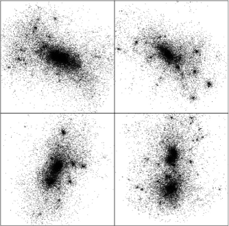
Figure 1.— Some cluster examples. The top left panel shows the most massive cluster in the simulation ($M=1.4\times 10^{15}{\rm h^{-1}M_{\odot}}$); top right: $M=8.3\times 10^{14}{\rm h^{-1}M_{\odot}}$; bottom left: $M=1.1\times 10^{15}{\rm h^{-1}M_{\odot}}$; bottom right: $M=1.2\times 10^{15}{\rm h^{-1}M_{\odot}}$. Each panel is $8\;h^{-1}{\rm Mpc}$ wide.

2.2. Cluster and Galaxy Selection

For group finding, we use the friends-of-friends (fof) method (e.g., Huchra & Geller 1982). A particle is defined to belong to a group if it is within some linking length ($b$) of any other particle in the group. We select clusters by using $b=0.2$ where $b$ is the linking length as a fraction of the mean particle separation. This definition of dark matter haloes was shown by Jenkins et al. (2001) to yield a mass function with a univeral form. Running the fof algorithm again, this time with $b=0.05$, we find the largest group in each cluster, and define this to be the most massive or central galaxy. When we refer to “galaxies” apart from the most massive galaxy later in the paper, we refer to particles randomly sampled from those cluster member particles which do not fall in the central galaxy halo.

In Figure 1 we show some examples of rare rich clusters selected from the simulation in this way. The most massive cluster in the entire simulation has mass $\sim 1.4\times 10^{15}{\rm h^{-1}M_{\odot}}$. Because the simulation includes non-linear clustering and clusters form from the bottom up, we expect each cluster to have its own substructure. Even though we are at $z=0$ and one might have expected some relaxation to have occurred, the substructure is very obvious. The cluster in the bottom right plainly consists of two clusters with similar masses merging. If such a merger was seen face on, then observationally it would be possible to separate the clusters. However, if the clusters lie one behind the other along the line of sight, this would not be possible. In analyzing our simulated clusters, we are conservative and do not assume that clusters with much substructure could be removed, so that we use all clusters selected with our fof algorithm.

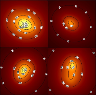
Figure 2.— Slices through the gravitational potential profile of different mass clusters (same as Figure 1). Contours are of gravitational redshift with respect to $\infty$ and are labelled in km/s.

2.3. Calculation of Gravitational Redshifts

As a measure of gravitational redshift, we adopt velocity units, so that the quantity is given by:

$$\Delta v_{g}=\Delta z_{g}c=\frac{\Delta\Phi}{c},$$ (2)

where $\Phi$ is the gravitational potential. For each particle in the simulation, we calculate the gravitational potential with respect to infinity using a tree algorithm (Barnes & Hut 1986). When doing this, we soften the gravitational potential in order to avoid noise from particles very close to one another, using 5 h^-1 Kpc equivalent Plummer softening (e.g., Aarseth 1963).

In Figure 2 we plot contours of gravitational redshift in some examples of galaxy clusters (the same clusters whose density distributions were shown in Figure  1.) Each panel shows the two dimensional slice of gravitational potential in the $xy$ plane that passes through the cluster center of mass. The substructure in the cluster density field is also somewhat reflected in the potential profile. However, the potentials are smoother, and even the merging clusters in the bottom right panel do not show strong evidence of two minima in the potential. The gravitational redshifts, which are related to the potential will therefore vary smoothly across the cluster, without much substructure. The substructure in the density distribution will however cause noise in the Hubble flow part of the total redshift (see §3.2).

Figure 3.— The effect of gravitational redshift for the most massive cluster. The line of sight lies parallel to the y-axis. The lines start at the position of a galaxy before adding its gravitational redshift and end at the position including the gravitational redshift. Peculiar velocities are not added in the plot.

In Figure 3 we show the effect of gravitational redshifts on the positions of particles when they are plotted in redshift space. We choose $y$ as the line of sight.In this figure we have not included the effect of peculiar velocities so that the much smaller gravitational redshift effect can be clearly seen. The value of $\Delta v_{g}$ for the central galaxy is $\sim 40km/s$, which causes it to be displaced $0.4\;h^{-1}{\rm Mpc}$ further away from the observer than in real space. The gravitational redshift gets smaller rapidly as we move away from the center of the cluster and particles at the edges of the cluster mass distribution have $\Delta v_{g}$ values wrt infinity of $\sim 5{\rm\;km\;s^{-1}}$.

3. Results

3.1. Comparison with an Analytic Profile

We compare the gravitational redshift from the simulation with an analytic prediction using a spherically symmetric density profile. We are interested in the difference in gravitational redshift between the central galaxy and the other cluster members and we will compare our analytic results with those from the simulation. The density profile we adopt is given by (Hernquist 1990):

$$\rho(r)\propto\frac{1}{r(a+r)^{3}}$$ (3)

where $a\sim R_{e}/1.8153$. The spatial gravitational redshift profile implied by this is (Cappi 1995):

$$V_{H}=\frac{GM}{c(r+a)}.$$ (4)

The gravitational redshift of the central galaxy or of the cluster is then given by integrating the mass weighted $V_{H}$ value over the radius of the galaxy or the radius of the cluster, as in the following expression:

$$v_{g}=\frac{\int^{r_{g}}_{0}\rho(r)V_{H}(r)dV}{\int^{r_{g}}_{0}\rho(r)dV}=\frac{GM}{c}\frac{\int^{r_{g}}_{0}\frac{r}{(a+r)^{4}}dr}{\int^{r_{g}}_{0}\frac{r}{(a+r)^{3}}dr},$$ (5)

where here $r_{g}$ is the galaxy radius.

We use the trapezoidal rule to integrate Eq. 5 numerically. For the characteristic radius of the central galaxies and the clusters, we take the mass weighted mean radius of galaxy (or cluster) member particles. With this definition, the average characteristic radius of clusters in the simulation with mass greater than $10^{13}\;h^{-1}{\rm Mpc}$ is 0.338 $\;h^{-1}{\rm Mpc}$, and the average radius of galaxies in those clusters is $0.084\;h^{-1}{\rm Mpc}$ With a threshold in mass of $10^{14}\;h^{-1}{\rm Mpc}$ the average radius of clusters and galaxies respectively is $0.713\;h^{-1}{\rm Mpc}$ and $0.154\;h^{-1}{\rm Mpc}$. The characteristic radius of the largest cluster in simulation is 1.9 $\;h^{-1}{\rm Mpc}$.

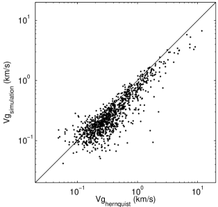
Figure 4.— Difference in gravitational redshift between the most massive galaxy and the rest of cluster members. $x$ axis: from Hernquist analytic profile using Eq 5, $y$ axis: from simulation. The straight line is where $Vg_{hernquist}=Vg_{simulation}$.

For the gravitational redshift of the most massive galaxy, Eq. 5 has been integrated up to the radius of the most massive galaxy, and for the gravitational redshift of the rest of members, the size of the most massive galaxy and the radius of the cluster are used as the lower and upper limits of integration respectively. The difference between the two values are calculated and the results from the simulation and from Eq. 5 are plotted in Figure 4. We can see from the figure that the values of central galaxy gravitational redshift from the simulation are broadly consistent with the estimate from analytic Hernquist density profile, although the estimate from analytic profile is slightly larger (by about $25\%$) than the result from the numerical simulation. We investigated if this could be due to the substructure of clusters, i.e., we checked whether $\Delta v_{g}$ is large when $\Delta y_{c.m.}$ is small, which might be expected if concentricity of the galaxy and cluster yields a greater gravitational redshift. We find no such effect, however. A possible explanation of the difference could follow from the known fact that the density profiles of halos are better fitted by the NFW profile which gives $\rho\propto 1/r^{3}$ for large $r$ rather than the steeper ($\rho\propto 1/r^{4}$) Hernquist profile. The latter would lead to a greater difference in the potential of the outer and central parts. In any case, the scatter we see in Figure 4 is quite small, indicating that substructure and deviations from spherical symmetry do not disrupt the agreement with the analytic results. Also apparent from the plot is the range of gravitational redshifts which will be relevant in our study, from $\sim 1{\rm\;km\;s^{-1}}$ to $\sim 10{\rm\;km\;s^{-1}}$.

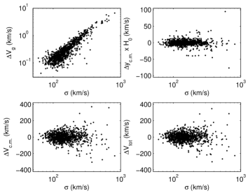
Figure 5.— The difference in gravitational redshift velocity (top left), center of mass (top right), and center of mass velocity (bottom left) of the central galaxy from the rest of the cluster members as a function of velocity dispersion. The bottom right panel shows the total redshift velocity, which is the sum of the 3 previous components. 1,000 randomly chosen clusters are shown.

3.2. Gravitational Redshift in Redshift Space

The total redshift velocity difference we observe between a galaxy and cluster is given by:

$$\Delta v_{tot}=\Delta v_{g}+\Delta y\times H_{0}+\Delta v,$$ (6)

where $\Delta y\times H_{0}$ is the Hubble expansion part and $\Delta v$ is the peculiar velocity. For each component, we have calculated the difference in redshift between the most massive galaxy and the other cluster members (see also §3.3). There will also be measurement errors on the redshift, which we shall cover later. In Figure 5 we plot each redshift component separately and the total redshift as a function of the cluster line-of-sight velocity dispersion. In order that these values may be related to cluster mass, we have fitted a power law to the relationship between cluster mass and velocity dispersion, finding it to be:

$$\log M=(2.56\pm 0.04)\log\sigma+7.12\pm 0.08,$$ (7)

where $M$ is in units of ${\rm h^{-1}M_{\odot}}$ and the units of $\sigma$ are ${\rm\;km\;s^{-1}}$. The slope of the relation is not too far from the value of 2 expected for virialized objects. The massive, high velocity dispersion clusters have the largest central galaxy gravitational redshifts. The rest of the redshift components exhibit larger scatter as velocity dispersion increases.

The cluster in the bottom right panel in Figure 1 has more substructure than the others and this is reflected in the large redshift difference between the most massive galaxy and the center of mass of rest of members. The position differences for all the panels are $\Delta y_{c.m.}=$ 0.0698, 0.049, -0.181 and 1.309 $\;h^{-1}{\rm Mpc}$ respectively (clockwise from the top left in Figure 1). Compared to the velocity difference, however, this has a small effect on the total redshift (see top right panel in Figure  5). Figure 5 shows that most scatter comes from the velocity difference between the central galaxy and the rest of the cluster.

The plot shows how small the gravitational redshift is compared to the other redshift components. In the bottom right panel of Figure 5 where we show the total redshift, it is obvious that we cannot see the effect of gravitational redshifts by eye on individual clusters or overall in a scatter plot such as this one.

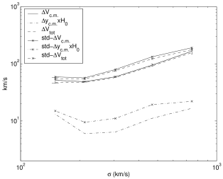
Figure 6.— Difference in redshift between central galaxy and cluster centroid as a function of cluster velocity dispersion $\sigma$. We show the scatter in center of mass velocity, Hubble component, and total redshift, as in Figure 5. The lines show the values which enclose 68% of the distribution and symbols the $1\sigma$ standard deviations. Error bars (Poisson errors) are shown for the center of mass velocity.

The redshift due to the position and velocity differences will be the most important source of noise when we try to extract the gravitational redshift. If the most massive galaxy were lying at rest at the centroid of the cluster, then the accuracy of our measurement of the gravitational redshift difference between it and the other cluster members would be limited only by Poisson noise in computation of the mean redshift of the cluster. Because the central galaxy is usually moving with respect to the mean of the other cluster members, and is usually not at the cluster center of mass, we have this additional source of noise, shown in the bottom left panel of Figure 5. Averaging results over many clusters in order to reduce the error on the mean $v_{g}$ is the approach we will take in this paper. An interesting question is how best to do this. For the clusters with the greatest mass, $v_{g}$ will be large, but so will the noise per cluster. On the other hand, $v_{g}$ for small mass clusters is small but the peculiar velocity and position noise is small as well. We will discuss this more later in the paper and determine the optimal range of cluster mass for detection of gravitational redshifts.

One can ask how one might expect the dominant noise component $\Delta V_{c.m.}$ to scale with the cluster velocity dispersion $\sigma$. If the central galaxy were a random galaxy in the cluster, then the scatter in $\Delta V_{c.m.}$ should be approximately $\sigma$. However, we expect it to be substantially less than this, as the central galaxy, while not at rest is still moving less with respect to the cluster center of mass than a random galaxy. In order to quantify this, we have plotted in Figure 6 the standard deviation of $\Delta V_{c.m.}$ against $\sigma$. We find standard deviation of $\Delta V_{c.m.}$ to be approximately $0.35\sigma$. We have also plotted the other source of noise from the Hubble component $\Delta y_{c.m.}\times H_{0}$, as well as the total, $\Delta V_{tot}$. Interestingly, the total noise on the central galaxy position, $\Delta V_{tot}$ is slightly lower than $\Delta V_{c.m.}$. On investigation, we have found that this is because of residual coherent infall of particles into the cluster, so that clusters on the far side, with +ve $\Delta y_{c.m.}\times H_{0}$ have -ve values of $\Delta V_{c.m.}$ and vice versa. In Figure 6, we also compare the directly computed $68\%$ interval to the standard deviation, finding that the distribution of $\Delta V_{tot}$ is close to Gaussian.

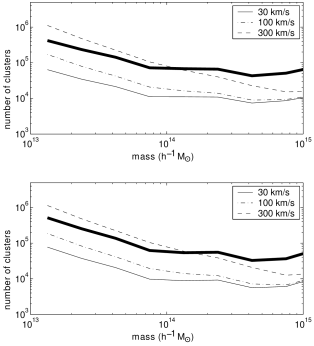
Figure 7.— The number of clusters needed to detect graviational redshift as a function of cluster mass. We show results using either 50 randomly selected galaxies per cluster (top) or using a number of galaxies proportional to the cluster mass (bottom), both for a 2$\sigma$ level detection. For the latter case, the number of galaxies used is equal to 0.1 times the number of dark matter particles in it, so that for a $10^{13}{\rm h^{-1}M_{\odot}}$ we use 15 galaxies. Measurement uncertainties of 30 km/s, 100 km/s and 300 km/s are included. The thick line represents a 4$\sigma$ detection with no measurement uncertainty. Note that the graph flattens for large cluster masses.

3.3. Estimate of the Number of Clusters Needed to Observe Gravitational Redshifts

One simple method for detection of gravitational redshifts would involve finding the redshift difference between the central galaxy and the other cluster members, after averaging over a large number of clusters. We have seen in the previous section that the noise from substructure is small, and that this should be feasible given enough clusters. In this subsection we investigate how well this could be done in practice. In the next subsection, we will include information on all galaxies in the cluster rather than just splitting the galaxy population into “central galaxy” and “other”.

With the difference in gravitational redshift computed from the simulation, we make an estimate of the number of clusters needed for a detection. We try two cases, randomly selecting either $N_{gal}=50$ galaxies per cluster or $N_{gal}$ = one tenth of the number of dark matter particles, so that $N_{gal}=M_{cluster}/7\times 10^{11}{\rm h^{-1}M_{\odot}}$. We assume that the noise from the difference in position and velocities contributes independently. Including the measurement uncertainty $\Delta_{meas.}$, we have

$$\sigma_{tot}^{2}=\sigma_{vel.}^{2}+\sigma_{pos.}^{2}+\Delta_{meas.}^{2},$$ (8)

where

$$\sigma_{vel}^{2}=\frac{1}{N_{c}-1}\sum_{i=1}^{N_{c}}(v_{i}-v_{gal,i})^{2}$$ (9)

and

$$\sigma_{pos.}^{2}=\frac{1}{N_{c}-1}\sum_{i=1}^{N_{c}}(r_{i}-r_{gal,i})^{2}\times H_{0}^{2}$$ (10)

And the error on the mean is given by

$$\frac{\sigma_{tot}}{\sqrt{N_{0}}},$$ (11)

We have split the clusters in the simulation into bins by mass, and $N_{c}$ here is the number of clusters in the simulation in a particular bin. For each bin we compute the number of clusters ($N_{0}$) actually needed for a detection of the gravitational redshift, with a given statistical significance. For example, for clusters in the mass bin centered on $\sim 8\times 10^{14}{\rm h^{-1}M_{\odot}}$, $\sigma\sim 300{\rm\;km\;s^{-1}}$ and $\Delta v_{g}\sim 7{\rm\;km\;s^{-1}}$. With $\sim 10^{4}$ clusters we expect our error bar to be $\sim 3{\rm\;km\;s^{-1}}$, which is a $\sim 2\sigma$ detection of gravitational redshift.

We might expect that the number of clusters should decrease for high mass because the gravitational redshift is proportional to the cluster velocity dispersion. However, for these clusters, the error bars also increase because the dispersion in velocity difference between central galaxy and others is getting larger. Figure 7 shows how many clusters we need to detect the gravitational redshift at the 2$\sigma$ and 4$\sigma$ levels as a function of cluster mass. We choose the measurement uncertainty to be 30 km/s, 100 km/s and 300 km/s as best, typical and worst cases (e.g., Stoughton et al. 2002). Given relatively small measurement uncertainty, the number of clusters needed decreases at first and then stays roughly the same ($\sim 10^{4}$ clusters for $\Delta_{meas.}=$ 30 km/s) after $M\lower 2.15277pt\hbox{$\;\buildrel>\over{\sim}\;$}10^{14}{\rm h^{-1}M_{\odot}}$. Since we use average values, it does not make much difference whether we use 50 galaxies per cluster or a number proportional to the cluster mass.

In order to understand the behaviour seen Fig 7, we can ask what should happen if the redshift noise on the central galaxy from peculiar velocities and position differences were proportional to the cluster velocity dispersion (assuming we are averaging over a fixed number of galaxies in each cluster). As the gravitational redshift is proportional to cluster velocity dispersion also (Figure 5), then the number of clusters for a detection of a given significance should be constant. This is approximately what is seen for clusters of mass $M$ greater than $\sim 10^{14}{\rm h^{-1}M_{\odot}}$. For smaller clusters, the noise from the displacement of the central galaxy (the Hubble velocity component, $\Delta y_{c.m.}\times H_{0}$) is becoming a non negligible fraction of the total noise, and its effect means that more clusters must be averaged over.

Note that, as mentioned above, only the mass-averaged gravitational redshift has been used here and it has not been taken into account that the gravitational redshift has a gradual radial dependence. More information is therefore available which could in principle aid a detection. We discuss this in the following subsection.

3.4. Gravitational Redshift Profile

We now calculate the profile of gravitational redshifts averaged over many clusters. As in the previous section, we take the central galaxy to be our zero point. The other galaxies in the cluster are binned as a function of their impact parameter from this galaxy ($r=\sqrt{\Delta x^{2}+\Delta z^{2}}$, where $y$ is the line of sight) In each bin, and for all clusters, we have summed the gravitational redshift difference between the galaxy and the central cluster galaxy. We then divide by the number of galaxies in each bin (as mentioned previously the “galaxies” which are not the central one are actually particles).

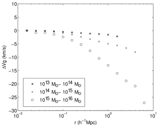
Figure 8.— The gravitational redshift profile averaged over many clusters as a function of impact parameter from the most massive galaxy. The gravitational redshift of the central galaxy is subtracted from the average gravitational redshift of the rest of cluster members.

Figure 8 shows the resulting gravitational redshift profile for clusters within different mass ranges as a function of the impact parameter $r$. All of the clusters in the simulation have been used, and it should be noted that each mass bin does not an have equal number of clusters contributing to it. Also, at large radii, within each mass range, only the more massive clusters contribute, because the smaller clusters do not have any galaxies out that far. As expected, gravitational redshifts increase for large mass clusters. This result is consistent with that of Cappi (1995) who used analytic profiles, in that the function decreases smoothly with a maximum at the center.

As we have described in section 3.1 our central galaxies have a mean radius of $\sim 0.1\;h^{-1}{\rm Mpc}$, which means that within the central few bins, we do not expect the gravitational redshifts of the galaxy to rise very steeply. If the central galaxy were modelled as a point (as was done by Broadhurst & Scannapieco 2000), the profile could become steeper. The dark matter halos in this simulation will have profiles consistent with the NFW form, so that we do not expect the central profile to be very steep even if the central galaxy is allowed to be much smaller, at least in this dark matter only run. The gravitational redshift profile for NFW clusters is shown in Broadhurst & Scannapieco 2000., and flattens off towards the center. According to El-Zant et al. (2003), any baryonic dissipational effects can cause either a steeping or flattening of the density profile towards the center, which will increase or decrease the gravitational redshift, but this is ignored in the present study.

In order to use the redshift profile information to make a detection of gravitational redshift, we must average over a large number of clusters to reduce the noise from peculiar velocities and Hubble expansion. As before, we add the total redshifts for many clusters so that the redshifts from position and velocity are averaged out, leaving only the gravitational redshift. This time, this will be done in bins of impact parameter. We can then estimate how many clusters we need to observe in order to ascertain to a given significance level that the gravitational redshift is inconsistent with zero.

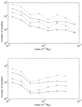
Figure 9.— top: Number of clusters needed to detect gravitational redshifts at the $2\sigma$ (circle) and $4\sigma$ ($\times$) levels as a function of cluster mass. The $\chi^{2}$ has been calculated with (dotted line) and without the (solid line) covariance matrix. We use all particles in each cluster. bottom: Number of clusters needed to detect gravitational redshifts as a function of mass when we are restricted to 100 galaxies per cluster. Note that the graph flattens for the mass above $\sim 3\times 10^{13}h^{-1}M_{\odot}$ when only diagonal terms are used. Measurement uncertainties are not included.

First, given a sample of simulated clusters in a certain mass range, we calculate the gravitational redshift profile in bins of impact parameter and the matrix of covariance between bins. The technique of Singular Value Decomposition (Press et al. 1992) is used to invert the matrix, and then the value of $\chi^{2}$ is computed:

$$\chi^{2}=\sum_{N}(x_{i}-\overline{x}_{i})C_{ij}^{-1}(x_{j}-\overline{x}_{j})$$ (12)

where $x_{i}$ is the gravitational redshift, $C_{ij}$ is covariance matrix. As we are interested in the possibility of detection, we set $\overline{x}_{i}=\overline{x}_{j}=0$ exactly so that $\chi^{2}$ is then the difference $\Delta\chi^{2}$ from a model with zero gravitational redshift. Because $C_{ij}$ is proportional to $1/\sqrt{N_{i}N_{j}}$, where $N_{i}$ is the number of clusters contributing to $r$ bin $i$, $\chi^{2}$ is proportional to the total number of clusters, if $N_{i}=N_{j}$. The number of $r$ bins which could be used depends on the angular extent of the cluster. Our criterion is to truncate at the outermost bin with less than 20 clusters contributing and not use the larger $r$ bins to build the covariance matrix. Additionally, when the number of clusters in a given mass range is small, the matrix is too noisy to invert. We consider the results invalid when $\chi^{2}$ calculated with the covariance matrix is greater than $\chi^{2}$ computed using only the diagonal elements of the covariance matrix. This occurs for the clusters with $M>5\times 10^{14}{\rm h^{-1}M_{\odot}}$ since there are only 4 in the simulation, and for this mass range we use the diagonal elements of the matrix only.

The top panel in Figure 9 shows the number of clusters needed for detections of non-zero gravitational redshifts at the 2$\sigma$ and 4$\sigma$ levels as a function of mass. No measurement uncertainties are included in this plot. $\chi^{2}$ values with only the diagonal elements were also calculated and those results are shown as additional lines in the plot. Including the proper covariances between bins reduces the sensitivity of the test, so that approximately a factor 2 more clusters are needed. The plot has slightly different behaviour to Figure 7, as the number of clusters needed continues to decrease for high masses. This is basically because we have used all galaxy information in each cluster. This is obviously not very realistic, as up to 20000 galaxies (particles) have been averaged over in the most massive clusters. We have therefore recomputed our results assuming that only 100 galaxies per cluster are available.

When we do this as shown in the bottom panel in Figure 9, we find that the curve flattens for high mass clusters and even goes up slightly when the effect of covariances is included. This means that observing clusters of mass $\sim 5\times 10^{13}{\rm h^{-1}M_{\odot}}$ seems to be the most efficient way to detect gravitational redshifts, at least when using galaxies as tracers of the potential. For higher mass clusters, we have larger gravitational redshift effects but also have more noise.

Note that when only the diagonal terms in the covariance matrix are used in $\chi^{2}$ calculation the flattening of the graph is consistent with the simpler estimator in §3.2 (Figure 7). However, both the mass threshold and the number of clusters needed to detect gravitational redshifts are smaller here, by about a factor of 3. This is because we have more information in the sense that we use the gravitational redshift profile in many $r$ bins while in §3.2, there are effectively only two bins - the central galaxy and the rest of the galaxies in each cluster.

For a more direct comparison with Figure 7, we then use 50 galaxies per cluster and one-tenth the number of particles while including measurement uncertainties in the covariance matrix (Figure 10). When the uncertainty is small, the result is consistent with Figure 7 in that with fixed number of galaxies per cluster, the curve flattens for high mass clusters. However, when the uncertainty is large, it appears that the measurement uncertainty is the dominant factor deciding the number of clusters needed regardless of the number of galaxies per cluster.

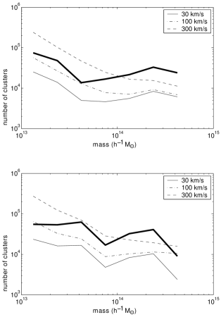
Figure 10.— top: Number of clusters needed to detect gravitational redshifts at the $2\sigma$ level as a function of cluster mass. The measurement uncertainties of 30 km/s, 100 km/s and 300 km/s are included. We use 50 particles per cluster (top) and tenth the size of cluster (bottom). Note that the graph flattens for the mass above $\sim 3\times 10^{13}h^{-1}M_{\odot}$. The thick line represents the $4\sigma$ level with no measurement uncertainty.

We have seen that for a $2\sigma$ detection of gravitational redshifts we expect to need a sample of $\sim 5000$ galaxy clusters/groups with 50 measured redshifts per cluster ( with measurement error $\Delta_{meas.}$ = 30 km/s). A statistically correct detection would involve making use of the covariance matrix of the noise between bins, which could be done from our model clusters, or else computed directly from the observational sample itself. This required number of clusters/groups is large, but may be just within the range of present day redshift surveys. We will return to this in our discussion (§5), as well as exploring results from a recent survey below. Alternatively, as stressed by Cappi (1995), the observed absence of an effect could be used to place limits on the gravitating mass of clusters.

4. Results from the ENACS survey

The ESO Nearby Abell Cluster Survey (ENACS, Katgert et al. 1998) is a redshift survey of rich Abell clusters in the southern sky. The catalog contains redshift, magnitude and position information for 5634 galaxies in 107 clusters. The mean velocity dispersion of these clusters is $\sim 700{\rm\;km\;s^{-1}}$ (Biviano et al 1996), so that based on the work in §3 we only expect there to be a small ($\sim 5{\rm\;km\;s^{-1}}$) redshift difference on average between the central galaxy and the other cluster members. We will compute this statistic in order to check consistency with our expectations.

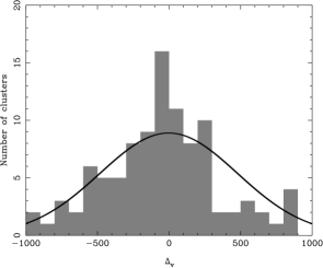
Figure 11.— Difference in redshift between the brightest cluster galaxy and the other cluster members, for 107 rich Abell clusters from the ENACS. A Gaussian curve with the same standard deviation, $\sigma=486{\rm\;km\;s^{-1}}$ is also shown.

We take the ENACS data and find cluster centers by placing a cylinder of length $3000{\rm\;km\;s^{-1}}$ along the line of sight and radius $2.0\;h^{-1}{\rm Mpc}$ around each galaxy. We find the center of mass of each cylinder (weighting each galaxy by the inverse of the selection function), recenter it on this point and iterate until convergence. We eliminate all overlapping cylinders, keeping those with most galaxies. We then rank all cylinders by the weighted number of galaxies and end up with a list of 107 rich clusters and their members.

Because we do not expect to be able to detect a gravitational redshift signal, we only carry out the simplest test, measuring the difference in redshift between the brightest galaxy in each cluster and the other cluster members. The results are shown as a histogram in Figure 11. The $rms$ difference between the brightest and other cluster galaxies is $486\pm 47{\rm\;km\;s^{-1}}$ (Poisson error). In the simulations, for a sample of clusters with the same mean velocity dispersion we expect an rms difference of $255{\rm\;km\;s^{-1}}$ (from Hubble flow and peculiar velocities.) This is rather lower than the observed value, and in fact it takes a simulated sample with a mean velocity dispersion of $970{\rm\;km\;s^{-1}}$ to have the same $rms$ difference (by applying a lower mass threshold of $9.3\times 10^{14}{\rm h^{-1}M_{\odot}}$. This could be a sign that there may some differences between the structure of observed and simulated clusters. It is likely that this is at least partly due to observational measurement errors, as the quoted uncertainties of $\sim 100{\rm\;km\;s^{-1}}$, when added in quadrature would increase the rms difference to $275{\rm\;km\;s^{-1}}$. The mean of the histogram for the ENACS clusters is $-66{\rm\;km\;s^{-1}}$ (a blue shift), with a $1\sigma$ uncertainty of $47{\rm\;km\;s^{-1}}$ so that as expected there is no detectable evidence for gravitational redshifts from this small sample.

We note that Cappi (1995) also carried out a similar same test with a sample of 42 clusters with cD galaxies, and found a small blue shift, $-39\pm 32$ km/s. Although in the ENACS sample we have simply measured the redshift difference of the brightest galaxy without regard to whether it is a true cD or not, we find essentially consistent results. On the other hand, Broadhurst and Scannapieco (2000) find a mean cD redshift of $260\pm 58{\rm\;km\;s^{-1}}$ for a sample of 8 clusters, of which 5 have cooling flows. This value is an order of magnitude larger than what we expect from our simulations. These authors have pointed out that the central potential could have been made steeper over time by cooling flows.

5. Summary and Discussion

We have explored the gravitational redshifts of galaxies in the potential wells of simulated galaxy clusters. In particular we have concentrated on the possibility of detecting gravitational redshifts from surveys of cluster galaxies. Our main findings are as follows:

• For clusters of $\sim 10^{15}{\rm h^{-1}M_{\odot}}$, the difference in redshift between the central galaxy and the other cluster members is $\sim 10{\rm\;km\;s^{-1}}$.

• The gravitational potential of clusters does not exhibit much substructure, even when the clusters are not relaxed. The most important source of noise on a measurement is from galaxy peculiar velocities.

• The most sensitive method for detecting gravitational redshifts with galaxy data is to use the gravitational redshift profile as a function of impact parameter.

• For a given number of galaxy redshifts measured, the most efficient strategy would be to target clusters of $\sim 5\times 10^{13}{\rm h^{-1}M_{\odot}}$, which have lower noise from galaxy peculiar velocities than more massive clusters.

• For a 2$\sigma$ detection, we require $\sim 5000$ clusters with $M>5\times 10^{13}{\rm h^{-1}M_{\odot}}$ when the measurement uncertainty is 30 km/s and $\sim 2500$ clusters when the measurement uncertainty is negligible.

Our result for the shape of the gravitational redshift profile are consistent with that of Cappi(1995) and Broadhurst and Scannapieco (200). However, the masses of clusters in our simulation are generally smaller than those used as examples by these authors. For example Cappi (1995) found that gravitational redshift with respect to infinity of the central regions of a cluster of mass $M=5\times 10^{15}{\rm h^{-1}M_{\odot}}$ to be $>100{\rm\;km\;s^{-1}}$ and predicted the effect for even more massive clusters with $M=10^{16}{\rm h^{-1}M_{\odot}}$ ($v_{g}\sim 300{\rm\;km\;s^{-1}}$). Unfortunately, even though the gravitational redshift in a cluster with mass $10^{16}{\rm h^{-1}M_{\odot}}$ is large, there is little chance of finding such a massive cluster in the Universe.

We can roughly estimate the number of clusters in the universe whose mass is $M=8\times 10^{14}{\rm h^{-1}M_{\odot}}$ or greater. First, we approximate the mass function of clusters given by (Bahcall & Bode, 2003) as a power law:

$$\log n(>M_{1.5,com}=8\times 10^{14}{\rm h^{-1}M_{\odot}})\approx-2z-6.75,$$ (13)

The comoving distance as a function of redshift is given by (e.g., Hogg 1999):

$$D=D_{H}\int^{z}_{0}\frac{dz^{\prime}}{E(z^{\prime})}$$ (14)

where $E(z)\equiv\sqrt{\Omega_{M}(1+z)^{3}+\Omega_{k}(1+z)^{2}+\Omega_{\Lambda}}$ and $D_{H}=3000\;h^{-1}{\rm Mpc}$. We take $\Omega_{M}=0.3$ and $\Omega_{\Lambda}=0.7.$ We then find the total number of clusters in the universe (up to $z=1$, although raising the $z$ limit makes essentially no difference) :

$$N=\int ndV=4\pi D_{H}^{3}\times 10^{-6.75}\int^{1}_{0}\frac{10^{-2z}}{E(z)}\left(\int^{z}_{0}\frac{dz^{\prime}}{E(z^{\prime})}\right)^{2}dz.$$ (15)

Integrating Eq. 15 numerically we find that there are only $\sim 600$ clusters ($M>8\times 10^{14}{\rm h^{-1}M_{\odot}}$) observable in the entire universe. We have seen, however in §3, that in any case the larger noise from peculiar velocities in more massive clusters makes a detection of gravitational redshifts problematic anyway. It might be better to use lower mass clusters in order to detect the gravitational redshift, even though effect is small.

As for observed samples of clusters with lower masses, the situation is more promising. For example, the Sloan Digital Sky Survey has been used to find $\sim 1,000$ clusters in total with $z<0.15$ and $M>5\times 10^{13}{\rm h^{-1}M_{\odot}}$ so far (Chris Miller, 2003, private communication). For a more on cluster finding in the SDSS, see Nichol (2003) and Annis et al. (2003). Published samples of SDSS clusters include those of Goto et al. (2002) and Bahcall et al. (2003b). Merchan and Zandivarez (2002) have constructed a galaxy group catalog from the 100K data release of the the 2dF galaxy redshift survey (refs). They find $\sim 1000$ clusters/groups with masses $M>5\times 10^{13}{\rm h^{-1}M_{\odot}}$. The final 2dF data release contains $\sim 2\times 10^{5}$ galaxies (Colless et al. 2003), which should enable construction of a group/cluster catalog with $\sim 2500$ members above this lower mass limit. As we have seen in §3.4, this may be close to the level required in order to make a $2\sigma$ detection of the gravitational redshift. A catalog of similar groups selected from the final SDSS survey might allow a 4 $\sigma$ detection.

Because the effect we are searching for is very small (a redshift on the order of a few km/s), we must be careful to consider possible systematic effects. The effects of peculiar velocities and cluster substructure have been included in our simulations, and averaging over large numbers of clusters produces reasonable results. One effect we have not included is full selection of clusters in redshift space. In the simulation, we simply define a cluster in real space with a linking length of our choice. In a survey, we select the clusters in redshift space and we include some contaminating galaxies behind and in front of each cluster that are not members. This would act to increase the noise, but not by much, as they will be heavily outnumbered by cluster members.

A real problem would be any effect which gives a systematically positive or negative redshift for the central galaxy with respect to the other galaxies. If we select cluster galaxies using a cone of constant angular size rather than a cylinder of fixed radius, then more contaminating galaxies will come from the larger volume behind the cluster than in front, and the average redshift of the galaxies apart from the central one will change. We have calculated the potential effect of this bias using the cluster-galaxy cross-correlation function data of Croft et al. (1999) to find the number of contaminating galaxies. We find a relative blueshift of $\sim 1{\rm\;km\;s^{-1}}$ for the central galaxy. This can be avoided simply by using a cylinder to select cluster members, however.

An additional potential problem which goes in the opposite direction is the fact that with a magnitude limited survey, the contaminating galaxies behind the cluster should be fewer in number because they are at a greater distance. The size of this effect depends on the steepness of the luminosity function of galaxies. It could also however easily be eliminated by applying a local volume limit in the vicinity of each cluster, rejecting galaxies which would be too faint when placed at the far edge of the cluster.

In this paper we have seen that realistically, gravitational redshifts are an extremely small effect, and that looking at the most massive galaxy clusters may not help in detection because the noise is much larger than for small clusters. If a detection is to be made using a galaxy survey, it will be important to carry out cross checks. For example, enough data needs to be a available that clusters can be divided by mass into more than one bin, to make sure that the effect is largest for the high mass clusters (even if the error bar is large). The more tracers of the clusters potential that are available, the better. Broadhurst & Scannapieco (2000) have shown that X-ray emission from intracluster gas could be used. Other probes of the potential could include using redshifts of intracluster planetary nebulae (e.g., Feldmeier et al. 2003).

It may be marginally possible to detect the gravitational redshift of cluster galaxies with the data available today. However, more surveys of greater scope have been imagined for the future. Someday this will provide us enough information to separate the gravitational redshift effect from total redshift.

We thank the anonymous referee for useful suggestions. RACC acknowledges support from the NASA-LTSA program, contract NAG5-11634.

References

- (1) Annis, J. et al., 2003, in preparation.
- (2) Aarseth, S. J., 1963, MNRAS, 126, 223
- (3) Bahcall, N. & Bode, P., 2003, ApJ, 588, L1-L4
- (4) Bahcall, et al. , 2003b, ApJS, in press, astro-ph/0305202
- (5) Barnes, J., Hut, P. 1986, Nature, 324, 446
- (6) Biviano, A., Giuricin, G., Katgert, P., Mazure, A., den Hartog, R., Dubath, P., Escalera, E., Focardi, P., Gerbal, D., Jones, B., Le Fevre, O., Moles, M., Perea, J., Rhee, G., 1996, Astrophysical Letters and Communications, 33, 157
- (7) Broadhurst, T., & Scannapieco, E., 2000, ApJ, 533L, 93
- (8) Cappi, A., 1995, A&A, 301, 6
- (9) Colless, M. et al., 2003, astro-ph/036571
- (10) Croft, R.A.C., Dalton, G.B., & Efstathiou, G., 1999, MNRAS305, 547
- (11) El-Zant, A., Hoffman, Y., Primack, J., Combes, F., Shlosman, I., 2003, astro-ph/0309412
- (12) Feldmeier, J. J.; Ciardullo, R., Jacoby, G. H., Durrell, P. R., 2003, ApJS, 145,65
- (13) Frenk, C.S.,Colberg, J.M., Couchman, H.M.P., Efstathiou, G., Evrard, A.E., Jenkins, A., MacFarland, T.J., Moore, B., Peacock, J. A., Pearce, F. R., Thomas, P. A., White, S. D. M., Yoshida, N., astro-ph/0007362.
- (14) Goto, T., Sekiguchi, M., Nichol, R. C.; Bahcall, N. A., Kim, R. S. J.; Annis, J., Ivezic, Z., Brinkmann, J.; Hennessy, G. S., Szokoly, G. P., Tucker, D. L., 2002, Astronomical Journal, 123, 1807
- (15) Hernquist, L., 1990, ApJ, 356, 359.
- (16) Hogg, D.W., astro-ph/9905116.
- (17) Huchra, J.P., Geller M.J., 1982, ApJ, 257, 423.
- (18) Katgert, P., Mazure, A., den Hartog, R., Adami, C., Biviano, A., Perea, J, 1998, Astronomy and Astrophysics Supplements, 129, 399.
- (19) Jenkins, A., Frenk, C. S., White, S. D. M., Colberg, J. M., Cole, S., Evrard, A. E., Couchman, H. M. P., Yoshida, N, 2001, MNRAS, 321, 372
- (20) Merchan, M., Zandivarez, A., MNRAS, in press, astro-ph/0204493.
- (21) Navarro, J. F., Frenk, C. S., White, S. D. M., 1997, ApJ, 490,493.
- (22) Nichol, R.C., 2003, in the Carnegie Observatories Astrophysics Series, Vol. 3: Clusters of Galaxies: Probes of Cosmological Structure and Galaxy Evolution, ed. J. S. Mulchaey, A. Dressler, and A. Oemler (Cambridge: Cambridge Univ. Press)
- (23) Nottale, L., 1976, ApJ, 208, L103.
- (24) Nottale, L., 1990, in Gravitational Lensing, Mellier, Y., Fort, B., G.Soucail eds., Springer-Verlag, p.29
- (25) Rood, H. J., Struble, M. F., 1982, ApJ, 252, L7.
- (26) Press, W. H., Teukolsky, S. A., Vetterling, W. T., Flannery, B. P., 1992, Numerical Recipes, (Cambridge: Cambridge Univ. Press)
- (27) Sand, D., Treu, T., Smith, G., Ellis, R., 2003, ApJ, submitted, astro-ph/0309465
- (28) Stiavelli, M., Setti, G., 1993, MNRAS, 262, L51.
- (29) Stoughton, C. et al., 2002, AJ, 123, 485