The metallicity-luminosity relation at medium redshift based on faint CADIS emission line galaxies

The emission line survey within the Calar Alto Deep Imaging Survey (CADIS) detects galaxies with very low continuum brightness by using an imaging Fabry-Perot interferometer. With spectroscopic follow-up observations of $\rm{M}_{\rm{B}}\ga-19$ CADIS galaxies using FORS2 at the VLT and DOLORES at TNG we obtained oxygen abundances of 5 galaxies at $z\sim 0.4$ and 10 galaxies at $z\sim 0.64$. Combining these measurements with published oxygen abundances of galaxies with $\rm{M}_{\rm{B}}\la-19$ we find evidence that a metallicity-luminosity relation exists at medium redshift, but it is displaced to lower abundances and higher luminosities compared to the metallicity-luminosity relation in the local universe. Comparing the observed metallicities and luminosities of galaxies at $z\la 3$ with Pégase2 chemical evolution models we have found a favoured scenario in which the metallicity of galaxies increases by a factor of $\sim 2$ between $z\sim 0.7$ and today, and their luminosity decreases by $\sim 0.5-0.9$ mag.

1 Introduction

In the local universe, metallicity is well correlated with the absolute luminosity (stellar mass) of galaxies (Skillman et al. skilm (1989), Zaritsky et al. zarit (1994), Richer & McCall richer (1995), Garnett et al. garnet (1997), Hunter & Hoffman hunter (1999), Melbourne & Salzer melb (2002), among others) in the sense that more luminous galaxies tend to be more metal rich. This metallicity-luminosity relationship is often attributed to the action of galactic superwinds: massive (more luminous) galaxies reach higher metallicities because they have deeper gravitational potentials which are better able to retain their gas against the building thermal pressures from supernovae, whereas low-mass systems eject large amounts of metal-enriched gas by supernovae-driven winds before high metallicities are attained (e.g., MacLow & Ferrara maclow (1999)). However, a greater degree of gas consumption in luminous galaxies and/or suppressed infall of low-metallicity or pristine gas may also play a major role (Pagel pagel97 (1997)).

Optical emission lines from Hii  regions have long been the primary mean of gas-phase chemical diagnosis in galaxies (see, e.g., the review by Shields shields (1990)). The advent of large telescopes and sensitive spectrographs has enabled direct measurement of the chemical properties in the ionized gas of cosmologically–distant galaxies with the same nebular analysis techniques used in local Hii regions. Distant galaxies subtend small angles on the sky, comparable to typical slit widths in a spectrograph. A typical ground-based resolution element of 1$\aas@@fstack{\prime\prime}$0 corresponding to a linear size of $\sim 6$ kpc at $z=0.5$ encompasses the entire galaxy at medium redshift; so galaxy spectra tend to be integrated spectra. The use of spatially-integrated emission line spectroscopy for studying the chemical properties of star-forming galaxies at earlier epochs has been explored by Kobulnicky et al. (kob99 (1999)). They concluded that spatially-integrated emission line spectra can reliably indicate the chemical properties of distant star-forming galaxies. They also found that, given spectra with sufficient signal-to-noise, the oxygen abundance of these galaxies can be measured to within $\pm 0.2$ dex using the $\rm R_{23}$ method, first suggested by Pagel et al. (pagel (1979)). The $\rm R_{23}$ method allows to derive metallicities also for faint galaxies where only prominent emission lines are observable (see more details in Sect. 4).

At medium redshift, all previous attempts to study the evolution of metallicity with cosmic time (Kobulnicky & Zaritzky kobzar (1999), Hammer et al. hammer (2001), Carollo & Lilly carol (2001), Contini et al. contini (2002)) have been based on continuum selected samples, the emission lines of which were identified using spectroscopy. Owing to magnitude-limited selection effects in these surveys, the samples of medium redshift galaxies for which metallicities were determined are biased towards luminous galaxies. Thus, for instance, the CFRS sample used by Carollo & Lilly (2001), selected by $I<22.2$, contains only bright galaxies ($M_{B}<-20$) at redshift $0.6\la z\la 1$, the continuum of which is dominated by an evolved stellar population.

Kobulnicky & Koo (kobko (2000)) found that star-forming Lyman-break galaxies at $z\sim 3$ are 2$-$4 mag more luminous than local spiral galaxies of similar metallicity, and thus are offset from the local luminosity-metallicity relation. Also Pettini et al. (pettini (2001)) found that Lyman break galaxies at $z\sim 3$ are significantly overluminous for their metallicities.

It seems therefore possible that the whole metallicity-luminosity relation is displaced to lower abundances at high or medium redshifts, ilustrating how galaxies participate in the chemical evolution process.

The Calar Alto Deep Imaging Survey (CADIS, Meisenheimer et al. meise98 (1998), meise03 (2004)) allows the selection of galaxies by their emission line fluxes detected via narrow-band (Fabry-Perot) imaging, regardless of their continuum brightness. Thus, CADIS can reach galaxies with very low continuum brightness (and absolute luminosity), i.e. galaxies which have such faint continuum that they are only detectable by their emission lines. Combining metallicities for such faint CADIS galaxies in several narrow redshift bins with published abundances for more luminous galaxies at medium $z$ we aim to establish the metallicity-luminosity relation for several look-back time bins in the range $0.3<z<1$. The metallicity-luminosity relation at different reshifts is a valuable probe of chemical galaxy evolution, and a consistency check for chemical evolution models.

This paper is structured in the following way: In Sect. 2 we describe how we select galaxies at $0.39\la z\la 0.65$ from the CADIS emission line sample in order to determine their metallicities by follow-up spectroscopy. In Sect. 3 we present the spectroscopic follow-up of such emission line galaxies. In Sect. 4 we compute oxygen abundances of the spectroscopic sample. Finally, in Sect. 5 we discuss the evolution of the metallicity-luminosity relation with redshift. The “concordance” cosmology with $\rm{H}_{0}=70$ km s^-1 Mpc^-1, $\Omega_{0}=0.3$, $\Omega_{\Lambda}=0.7$ is used throughout this paper. For the solar oxygen abundance we use the value $12+\rm{log}(\rm{O/H})=8.87$ from Grevesse et al. (grevesse (1996)). Note that “metallicity” and “abundance” normally denotes “oxygen abundance” throughout this paper.

2 Selection of emission line galaxies at medium redshift from CADIS

CADIS combines a moderately deep multi-band survey (10 $\sigma$ limit, R${}_{\rm{lim}}=24$) with a deep emission line survey employing an imaging Fabry-Perot-Interferometer ($\rm{F}_{\rm{lim}}=3\cdot 10^{-20}\rm{W}\rm{m}^{-2}$), which covers three waveband windows (henceforth called FP windows) essentially free of atmospheric OH emission lines: A ($\lambda=702\pm 6$ nm), B ($\lambda=819\pm 5$ nm), and C ($\lambda=920\pm 8$ nm). An emission line detected in the Fabry-Perot scan can be any of the prominent nebular lines, e.g., Ly-$\alpha$, ${\rm[O\,II]\,}{\lambda\,3727}$, ${\rm H}{\beta}$, ${\rm[O\,III]\,}{\lambda\,5007}$, or ${\rm H}{\alpha}$. The line identification is done by means of the line profile, by fitting template galaxy spectra to the observed multi-filter SED, and by considering the flux in “veto-filters” at the expected wavelengths of other lines (Hippelein et al. hippe (2003), Meisenheimer et al meise03 (2004)).

The analysis of FP window A and B is nearly completed in four of the 6 CADIS fields with FP observations (Table 1 in Maier et al. maier03 (2003)). In these four CADIS fields we have found 128 galaxies by their ${\rm[O\,III]\,}{\lambda\,5007}$  emission detected in the FP windows A or B; they have redshifts in the redshift bin $0.392<z<0.415$, and $0.625<z<0.648$, respectively. Figures 1 and 2 show two examples of galaxies detected by their ${\rm[O\,III]\,}{\lambda\,5007}$  emission line in the FP scan. The ${\rm[O\,III]\,}{\lambda\,5007}$  line of the galaxy 23h-671455 (Fig. 1) is detected in the FP window A, and we see the ${\rm[O\,II]\,}{\lambda\,3727}$  emission line in the veto-filter at 522 nm. Moreover, ${\rm H}{\alpha}$  and the ${\rm[N\,II]\,}{\lambda\lambda\,6548,6584}$  doublet are seen in window C. For the galaxy 01h-584247 (Fig. 2), the ${\rm[O\,III]\,}{\lambda\,5007}$  line is seen by the Fabry-Perot in window B, and we detect the ${\rm[O\,II]\,}{\lambda\,3727}$  line in the veto-filter at 611 nm.

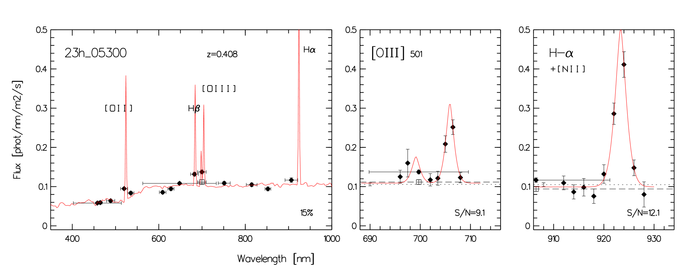
Figure 1: The galaxy 23h-671455 at $z\approx 0.41$: Photometry in all 14 optical CADIS filters fitted by a continuum-model with overlayed prominent emission lines (left panel), the Fabry-Perot measurements in window A with a [OIII] doublet profile fitted to the observed flux data (center), and the Fabry-Perot measurements in window C with a ${\rm H}{\alpha}$  $+$ ${\rm[N\,II]\,}{\lambda\lambda\,6548,6584}$  three-line profile fitted to the observed flux data (right panel). Note that the ${\rm[O\,II]\,}{\lambda\,3727}$  line is seen in the veto-filter at 522 nm. The numbers in the lower right edges of the right panels specify the signal-to-noise ratios, $F_{line}/\sigma_{line}$; $F_{line}$ and $\sigma_{line}$ are derived by fitting the Fabry-Perot instrument profile to the observed flux data points; see also Hippelein et al. (hippe (2003)).

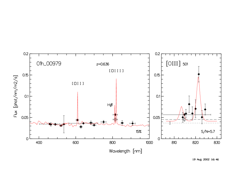
Figure 2: The galaxy 01h-584247 at $z\approx 0.64$: Photometry in all 14 optical CADIS filters fitted by a continuum-model with overlayed prominent emission lines (left panel), and the Fabry-Perot measurements in window B with a [OIII] doublet profile fitted to the observed flux data (right panel). Note that the ${\rm[O\,II]\,}{\lambda\,3727}$  line is seen in the veto-filter at 611 nm.

From the sample of 128 objects detected by their ${\rm[O\,III]\,}{\lambda\,5007}$  line in FP windows A or B we selected emission line galaxies for spectroscopic-follow up in order to determine their metal abundances. Oxygen lines are the most useful for measuring the abundance, since all important ionization stages can be observed. The temperature-sensitive ${\rm[O\,III]\,}{\lambda\,4363}$ line is often too weak to be measured even in the local universe (${\rm[O\,III]\,}{\lambda\,4363}$/${\rm[O\,III]\,}{\lambda\,5007}$  $\la 1/50$). To overcome this problem, Pagel et al. (pagel (1979)) suggested the empirical abundance indicator

$$\mbox{$\rm R_{23}$}=\frac{\rm{I}(\mbox{${\rm[O\,II]\,}{\lambda\,3727}$})+\rm{I}(\mbox{${\rm[O\,III]\,}{\lambda\lambda\,4959,5007}$})}{\rm{I}(\mbox{${\rm H}{\beta}$})}$$ (1)

for faint objects, such as galaxies at high redshift. The method has been later refined by McGaugh (mcgaugh (1991)) using a set of photoionisation models, and observationally confirmed to be reliable by Kobulnicky et al. (kob99 (1999)). For the 128 selected objects the ${\rm[O\,III]\,}{\lambda\,5007}$  line is measured in the respective Fabry-Perot window, while ${\rm H}{\beta}$  must be measured by spectroscopic follow-up, and ${\rm[O\,II]\,}{\lambda\,3727}$  is detected by a veto filter at 522 or 611 nm. However, since the determination of the ${\rm[O\,II]\,}{\lambda\,3727}$  flux relies only on a medium band filter, this flux is often not accurate enough to determine oxygen abundances with the $\rm R_{23}$  relation. Therefore, spectroscopic follow-up is necessary to measure not only the ${\rm H}{\beta}$  line, but also ${\rm[O\,II]\,}{\lambda\,3727}$. Since the ${\rm[O\,III]\,}{\lambda\lambda\,4959,5007}$  and ${\rm H}{\beta}$  lines lie close in wavelength to each other, the accurate fluxes of the ${\rm[O\,III]\,}{\lambda\lambda\,4959,5007}$  lines are provided for free by the spectroscopic follow-up.

From our 128 objects detected by their ${\rm[O\,III]\,}{\lambda\,5007}$  emission line seen in the Fabry-Perot we obtained spectra of 21 objects with absolute magnitudes fainter than $\rm{M}_{\rm{B}}\approx-19$, which were able to be placed on the slitmasks together with Ly-$\alpha$ candidates (Maier et al. maier03 (2003)) in order to maximize the number of galaxies observed; see Section 3 for the details of the observations. The large wavelength coverage of the CADIS filters allows to derive precise absolute magnitudes without using any K-correction factor, since the flux value at the restframe wavelength is calculated by linear interpolation between the measurements of two adjacent filters. In order to extend the sample of already published metallicities of galaxies at medium redshift to fainter absolute magnitudes, we selected for the spectroscopic follow-up objects with $\rm{M}_{\rm{B}}\ga-19$. We removed five objects from this sample because the ${\rm H}{\beta}$  line had too low signal-to-noise ratio for reliable oxygen abundance determinations (see Kobulnicky et al. kob99 (1999) for the discussion of the signal-to-noise required in order to get reliable metallicity measurements with the $\rm R_{23}$  method). The remaining 16 galaxies are listed in Table 2. As shown in Fig. 3, this final sample is only slightly biased towards special F(${\rm[O\,III]\,}{\lambda\,5007}$)/F(${\rm[O\,II]\,}{\lambda\,3727}$) ratios – a ratio which decreases with metallicity (Stasinska & Leitherer stasinsk (1996)) – in the sense that objects with F(${\rm[O\,III]\,}{\lambda\,5007}$)/F(${\rm[O\,II]\,}{\lambda\,3727}$) $<1$ are underrepresented (28% in the full sample, 12% in the spectroscopic sample).

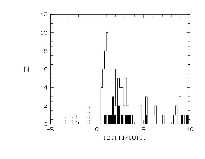
Figure 3: The histogram of F(${\rm[O\,III]\,}{\lambda\,5007}$)/F${\rm[O\,II]\,}{\lambda\,3727}$) flux ratios (as determined by the CADIS filter and Fabry-Perot measurements) of 128 emission line galaxies selected by their ${\rm[O\,III]\,}{\lambda\,5007}$  line seen in the Fabry-Perot; the filled boxes show the CADIS flux ratios for the galaxies with follow-up spectroscopy listed in Table 2. Note that the negative values (dotted lines) come from the fact that, for galaxies with undetectable ${\rm[O\,II]\,}{\lambda\,3727}$  flux, the uncertainties in the interpolated continuum and the background noise place the formally measured F(${\rm[O\,II]\,}{\lambda\,3727}$) flux symmetrically around F(${\rm[O\,II]\,}{\lambda\,3727}$)$=0$.

3 Spectroscopic observations

The spectroscopic follow-up observations of emission line galaxies in two redshift bins, at $0.392\la z\la 0.415$, and at $0.625\la z\la 0.648$, in the CADIS 01h- and 23h-fields were obtained in the summer and autumn of 2001, and in the summer of 2002, using FORS 2 at the VLT. Galaxies in 09h-field, and one galaxy in 01h-field at $z\approx 0.64$ (01h-5085) were observed with the Low Resolution Spectrograph DOLORES at Telescopio Nazionale Galileo (TNG). The slitmasks contained 1$\aas@@fstack{\prime\prime}$0 up to 1$\aas@@fstack{\prime\prime}$6 wide slits; the length of the slits varied between 10$\aas@@fstack{\prime\prime}$0, and 20$\aas@@fstack{\prime\prime}$0. Since we found from our first observations that the 1$\aas@@fstack{\prime\prime}$0 slit may miss (part of) the line emitting region (see discussion in Maier et al. maier03 (2003)), we used wider slits (up to 1$\aas@@fstack{\prime\prime}$6) for the observations with TNG (masks e, f), and for the VLT observations in summer 2002 (masks d, i).

Table 1: Spectroscopic follow-up observations.

Field	Mask	t(sec)	Grism	Res.(nm/slit)	Slitwidth	Inst./Telescope
01h	a	12860	300I	1.2	1′′.0	FORS2/VLT
01h	b	12500	600RI	0.8	1′′.0	FORS2/VLT
01h	b	7500	600R	0.5	1′′.0	FORS2/VLT
01h	c	6085	600RI	0.8	1′′.0	FORS2/VLT
01h	c	1700	600R	0.5	1′′.0	FORS2/VLT
01h	d	15750	300I	1.7	1′′.4	FORS2/VLT
01h	e	6000	LRR	1.2	1′′.1	DOLORES/TNG
09h	f	15600	HRR	0.5	1′′.6	DOLORES/TNG
09h	f	3000	MRB	1.0	1′′.6	DOLORES/TNG
23h	g	16080	300I	1.2	1′′.0	FORS2/VLT
23h	h	9000	600RI	1.8	1′′.0	FORS2/VLT
23h	i	15750	300I	1.7	1′′.4	FORS2/VLT

For the VLT observations we used three different grisms, the lower resolution 300 I grism, which gives a spectral resolution of about 1.2 nm at 800 nm for 1$\aas@@fstack{\prime\prime}$0  wide slitlets; the 600 RI grism, which gives a higher spectral resolution of about 0.8 nm at 800 nm for 1$\aas@@fstack{\prime\prime}$0  wide slitlets, and the 600R grism, which gives a spectral resolution of about 0.5 nm FWHM at 600 nm. However, since the objects have to be put on the masks according to the wavelength range to be observed, the 600RI grism has a smaller spectroscopically field-of-view than the 300 I grism, and thus allows less freedom in target positions. Moreover, one can measure only the ${\rm[O\,III]\,}{\lambda\lambda\,4959,5007}$  and ${\rm H}{\beta}$  lines of a galaxy at $z\approx 0.64$, and, in order to get ${\rm[O\,II]\,}{\lambda\,3727}$, the 600R grism has to be used additionally.

Spectra were reduced using the package LONG provided by MIDAS. Images were bias-subtracted first. In order to remove the low spatial frequencies along the dispersion axis from the flatfield, we averaged the original image along the slit, fitted the resulting one-dimensional image by a polynomial of second order, and divided the original flatfield by this image to obtain a normalized flatfield. Every mask contained about 20 single spectra. Every single spectra was extracted, treated as a long slit spectra, and divided through the respective normalized flatfield. For the wavelength calibration night sky lines were used, which have the advantage to be taken with the telescope and spectrograph in the same orientation as the science spectra. The one-dimensional spectra of each object were extracted with an aperture of about 10 pixels, i.e., about 2^′′, using the algorithm by Horne (horne (1986)). Fluxes were calibrated from digital units (ADUs) to physical flux units (W m^-2 s^-1 Å ^-1) using multiple observations of the spectrophotometric standard stars LTT 7379, EG 274, and LTT 7987 (Hamuy et al. hamuy92 (1992), hamuy94 (1994)).

For the observations with TNG we used the HRR and MRB grisms for galaxies at $z\approx 0.4$, and the LRR grism for the galaxy 01h-5085 at $z\sim 0.64$. Data reduction of the spectra was performed similar to the VLT data reduction. For the flux calibration the spectrophotometric standard star HD93521 (Oke oke (1990)) was used. Table 1 lists the details of the observations with the VLT and TNG.

4 Flux ratios and oxygen abundances

4.1 Emission line measurements

Emission line fluxes were measured interactively using the integrate/line routine in MIDAS. The flux error is calculated as $\sqrt{N}\times\sigma$, where $N$ is the number of pixels summed in a given emission line, and $\sigma$ is the root-mean-squared variation in a region of the spectrum next to the emission line. This yields typical errors of 5% for ${\rm[O\,III]\,}{\lambda\,5007}$, ${\rm[O\,III]\,}{\lambda\,4959}$, and ${\rm[O\,II]\,}{\lambda\,3727}$, and 5% to 12 % for ${\rm H}{\beta}$, depending on the position of ${\rm H}{\beta}$  between the night sky lines.. The error of $\rm R_{23}$  is thus dominated by ${\rm H}{\beta}$. Flux ratios were corrected for underlying Balmer absorption with a general ${\rm H}{\beta}$  absorption equivalent width of 2Å , representative of local irregular, HII, and spiral galaxies (see e.g., McCall et al. mccall (1985), Skillman & Kennicutt skillm93 (1993), Izotov et al. izo94 (1994)), and in agreement with the newest results for ${\rm H}{\beta}$  absorption equivalent widths from the study of about 600 SDSS strong emisison line galaxies (Kniazev et al. kniazev (2004)).

4.2 Extinction

The dereddened value for a flux line ratio, $\rm{I}(\lambda 1)/\rm{I}(\lambda 2)$, is given by:

$$\frac{\rm{I}(\lambda 1)}{\rm{I}(\lambda 2)}=\frac{\rm{F}(\lambda 1)}{\rm{F}(\lambda 2)}\times 10^{c(f(\lambda 1)-f(\lambda 2))},$$ (2)

where $\rm{F}(\lambda)$ is the observed flux at a given wavelength, c is the logarithmic reddening parameter that describes the amount of reddening relative to ${\rm H}{\beta}$, and $f(\lambda)$ is the wavelength-dependent reddening function (Whitford whitford (1958)). The value of c can be extimated from the relation $c=1.47\times\rm{E}_{\rm{B-V}}$ from Seaton (seaton (1979)).

The ratio $\rm{I}(\mbox{${\rm[O\,III]\,}{\lambda\,5007}$})/\rm{I}(\mbox{${\rm H}{\beta}$})$ which goes into the $\rm R_{23}$  relation is:

$$\frac{\rm{I}(\mbox{${\rm[O\,III]\,}{\lambda\,5007}$})}{\rm{I}(\mbox{${\rm H}{\beta}$})}=\frac{\rm{F}(\mbox{${\rm[O\,III]\,}{\lambda\,5007}$})}{\rm{F}(\mbox{${\rm H}{\beta}$})}\times 10^{-0.034\,c}.$$ (3)

Thus, since the ${\rm[O\,III]\,}{\lambda\lambda\,4959,5007}$  and ${\rm H}{\beta}$  lines lie close in wavelength to each other, the extinction is small and can be neglected for the $\rm{I}(\mbox{${\rm[O\,III]\,}{\lambda\,5007}$})/\rm{I}(\mbox{${\rm H}{\beta}$})$ ratio (the same applies also to the $\rm{I}(\mbox{${\rm[O\,III]\,}{\lambda\,4959}$})/\rm{I}(\mbox{${\rm H}{\beta}$})$ ratio).

The other ratio, $\rm{I}(\mbox{${\rm[O\,II]\,}{\lambda\,3727}$})/\rm{I}(\mbox{${\rm H}{\beta}$})$, which goes into the $\rm R_{23}$  relation is

$$\frac{\rm{I}(\mbox{${\rm[O\,II]\,}{\lambda\,3727}$})}{\rm{I}(\mbox{${\rm H}{\beta}$})} = \frac{\rm{F}(\mbox{${\rm[O\,II]\,}{\lambda\,3727}$})}{\rm{F}(\mbox{${\rm H}{\beta}$})}\times 10^{0.308\,c}$$ (4)

$$=\frac{\rm{F}(\mbox{${\rm[O\,II]\,}{\lambda\,3727}$})}{\rm{F}(\mbox{${\rm H}{\beta}$})}\times\alpha,$$

with $\alpha=10^{0.308\,c}$. Thus, the effect of reddening in the $\rm R_{23}$  expression can be written as:

$$\mbox{$\rm R_{23}$}\,=\frac{\alpha\times\rm{F}(\mbox{${\rm[O\,II]\,}{\lambda\,3727}$})+\rm{F}(\mbox{${\rm[O\,III]\,}{\lambda\lambda\,4959,5007}$})}{\rm{F}(\mbox{${\rm H}{\beta}$})}.$$ (5)

Assuming case B Balmer recombination, with a temperature of 10 000 K, and a density of 100 ${\rm{cm}}^{-3}$ (Brocklehust brockle (1971)), the predicted dereddened intensity ratio of ${\rm H}{\alpha}$  to ${\rm H}{\beta}$  is 2.86 (Osterbrock osterb (1989)). The effect of reddening on the ratio ${\rm H}{\alpha}$/${\rm H}{\beta}$  can be written as $\rm{I}(\mbox{${\rm H}{\alpha}$})/\rm{I}(\mbox{${\rm H}{\beta}$})=\rm{F}(\mbox{${\rm H}{\alpha}$})/\rm{F}(\mbox{${\rm H}{\beta}$})\times 10^{(-0.332)c}$. Using the spectroscopic follow-up measurements of the ${\rm H}{\alpha}$  line for three galaxies at $z\approx 0.4$ (see, e.g., Fig. 5), and the CADIS Fabry-Perot measurements of the ${\rm H}{\alpha}$  line available in window C for galaxies at $z\approx 0.4$ (see Fig. 1), the values of $c$ for the 5 galaxies at $z\approx 0.4$ are of order of $0-0.1$, yielding a value of $\alpha$ in the range 1 to 1.07. This means that the extinction (see equation 5) can be neglected with respect to the errors for the faint emission line galaxies ($\rm{M}_{\rm{B}}\ga-19$) at $z\approx 0.4$, when calculating $\rm R_{23}$. We assume that the same is true for galaxies with $\rm{M}_{\rm{B}}\ga-19$ in the redshift bin $0.625<z<0.645$.

This assumption is supported by the fact that the ${\rm[O\,III]\,}{\lambda\,5007}$  line flux is larger than the ${\rm[O\,II]\,}{\lambda\,3727}$  line flux for the 11 galaxies at $z\approx 0.64$ of our sample (see Table 2). Therefore, even allowing for a wider range $1<\alpha<2$ and typical large F(${\rm[O\,III]\,}{\lambda\,5007}$)/F(${\rm[O\,II]\,}{\lambda\,3727}$) ratios, equation 5 shows that the ${\rm[O\,III]\,}{\lambda\lambda\,4959,5007}$  and ${\rm H}{\beta}$  measurement errors, and not the unknown value of $\alpha$, dominate the error of the $\rm R_{23}$  ratio. Therefore, we do not correct the line fluxes for extinction for the galaxies in our sample.

4.3 The $\rm R_{23}$ relation

Because the temperature-sensitive line ${\rm[O\,III]\,}{\lambda\,4363}$  is not detectable in the spectra of galaxies at $z\ga 0.4$, the oxygen abundance has to be determined using the empirical calibration between oxygen abundance and $\rm R_{23}$. Pagel et al. (pagel (1979)) noted, based on a sample of extragalactic H II regions, that the measured T_e, O/H and $\rm R_{23}$ were all correlated. This works because of the relationship between O/H and nebular cooling: For metal-rich regions, the cooling in the ionized gas is dominated by emission in IR fine-structure lines (primarily the [O III] 52 $\mu$m and 88 $\mu$m lines), so as O/H increases, the nebula becomes cooler. In response to that, the highly excited optical forbidden lines, the [O III] lines, become weaker as O/H increases (excitation goes down as T decreases). At very high abundances, $12+\rm{log}(\rm{O/H})\ga 8.7$, Hii  regions are very cold ($T_{e}<6000$ K) and values of $\rm R_{23}$  are small. For $12+$log (O/H) $\la 8.2$, the relation between $\rm R_{23}$ and O/H reverses, such that $\rm R_{23}$ decreases with decreasing abundance. This occurs because at very low metallicities the IR fine-structure lines no longer dominate the cooling because of the lack of heavy elements. As a result, the forbidden lines reflect the abundance in the gas almost in a proportional way.

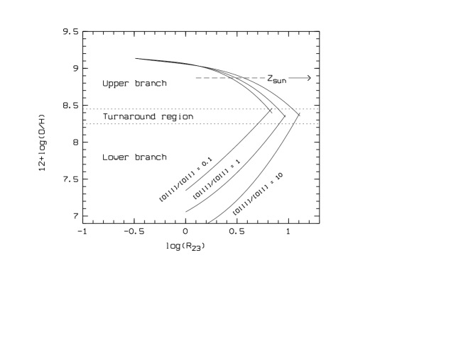
Figure 4: The oxygen abundance 12+log(O/H) as a function of the line ratio $\rm{log}\,\rm{R}_{23}$. The calibration between $\rm{R}_{23}$ and O/H (solid lines) using the models from McGaugh (mcgaugh (1991)) shows the effect of varying the ionization parameter in terms of the observable line ratio ${\rm[O\,III]\,}{\lambda\lambda\,4959,5007}$/${\rm[O\,II]\,}{\lambda\,3727}$ . On the lower, metal-poor branch, the ionization parameter becomes important. The ratio [O III]/[O II] of 10, 1.0, and 0.1 correspond (very roughly) to ionization parameters U of $10^{-1},10^{-2}$, and $10^{-4}$. The two horizontal dotted lines separate the different regions of oxygen abundances. The arrow and the horizontal dashed line indicate the solar oxygen abundance of $12+\rm{log}(\rm{O/H})=8.87$ (Grevesse et al. grevesse (1996)).

As a consequence, the $\rm R_{23}$  indicator is not a monotonic function of oxygen abundance (see Figure 4). At a given value of $\rm R_{23}$, there are two possible choices of the oxygen abundance. Roughly, the low abundance or “lower branch” is defined by $12+\rm{log}(\rm{O/H})\la 8.2$, whereas the high abundance or “upper branch” is defined by $12+\rm{log}(\rm{O/H})\ga 8.5$. Therefore, an additional indicator (e.g., the ${\rm[N\,II]\,}{\lambda\,6584}$  line) is needed in order to resolve the degeneracy in $\rm R_{23}$. About 50% of the emission line galaxies in our sample have log$\rm R_{23}$ in the range $0.8-1$ placing these galaxies in the “turnaround” region $8.2<12+\rm{log}(\rm{O/H})<8.5$ of the oxygen abundance versus $\rm R_{23}$  diagram (see Fig. 4). For the remaining galaxies we describe in the following how the decision, whether a galaxy lies on the upper or on the lower branch, has been taken.

4.3.1 Breaking the $\rm R_{23}$  degeneracy by the ${\rm[N\,II]\,}{\lambda\,6584}$/${\rm H}{\alpha}$ ratio

The ${\rm[N\,II]\,}{\lambda\,6584}$/${\rm H}{\alpha}$  line ratio can be used to break the degeneracy of the $\rm R_{23}$  relation, if one is able to measure and separate ${\rm[N\,II]\,}{\lambda\,6584}$  from ${\rm H}{\alpha}$. Denicolo et al. (denicolo (2002)) calibrated the N2 estimator, defined as N2 $=\rm{log}(I(\mbox{${\rm[N\,II]\,}{\lambda\,6584}$})/I(\mbox{${\rm H}{\alpha}$}))$, vs. the oxygen abundance, using a sample of Hii  galaxies having accurate oxygen abundances, plus photoionization models covering a wide range of abundances.

When the secondary production of nitrogen dominates, at somewhat higher metallicity, the line ratio ${\rm[N\,II]\,}{\lambda\,6584}$/${\rm H}{\alpha}$  increases with oxygen abundance. At very low metallicity, N2 scales simply as the nitrogen abundance to first order. However, in this metallicity regime, the nitrogen abundance shows a large scatter relative to the oxygen abundance, since the nitrogen abundance is much more sensitive to the history of star formation in the galaxy considered. As a result, N2 is probably not very useful to estimate oxygen abundance except as a means of determining the branch for the application of the $\rm R_{23}$  method. The division between the upper and the lower branch of the $\rm R_{23}$  relation occurs around ${\rm[N\,II]\,}{\lambda\,6584}$ /${\rm H}{\alpha}$  $\sim 0.1$. ${\rm[N\,II]\,}{\lambda\,6584}$ /${\rm H}{\alpha}$  line ratios were measured by follow-up spectroscopy for three CADIS galaxies at $z\approx 0.4$. 09h-448495 has an ${\rm[N\,II]\,}{\lambda\,6584}$ /${\rm H}{\alpha}$  line ratio $>0.1$, placing this galaxy on the upper branch of the $\rm R_{23}$  relation; the galaxy 23h-671455 has a ${\rm[N\,II]\,}{\lambda\,6584}$ /${\rm H}{\alpha}$  line ratio of $\sim 0.1$ and lies in the turnaround region; and 23h-683506 has a ${\rm[N\,II]\,}{\lambda\,6584}$ /${\rm H}{\alpha}$  line ratio $<0.1$, placing this galaxy on the lower branch of the $\rm R_{23}$  relation (see spectrum in Figure 5, lower panel).

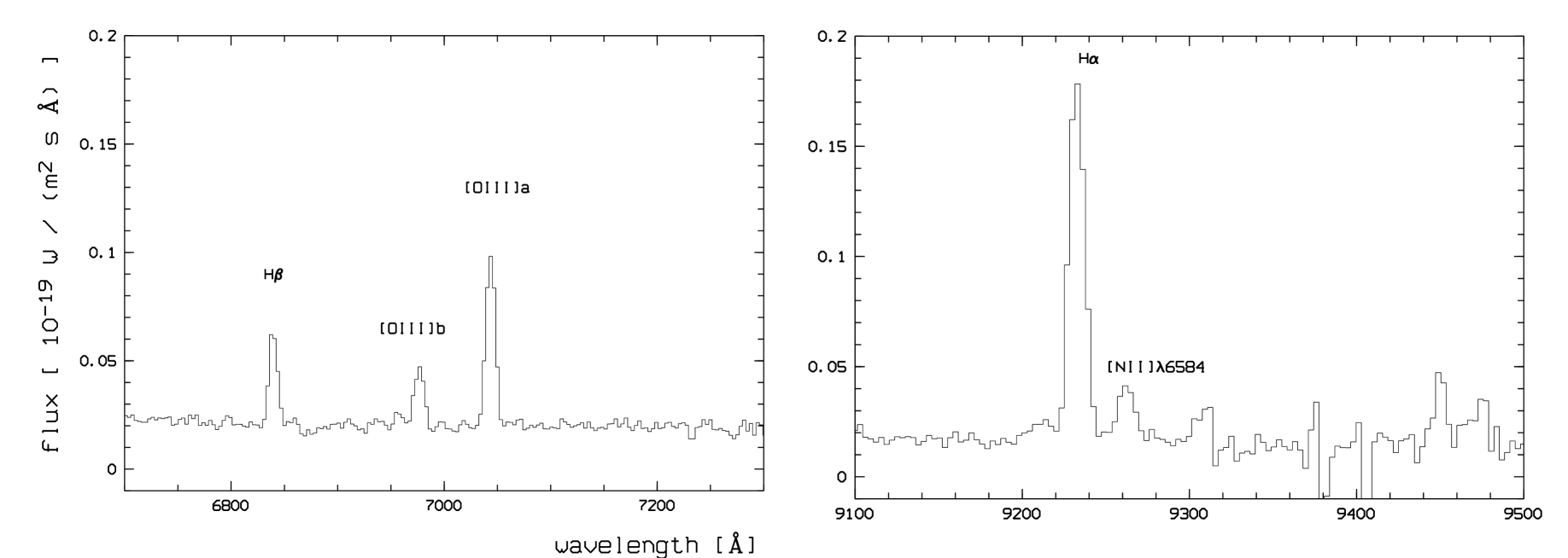
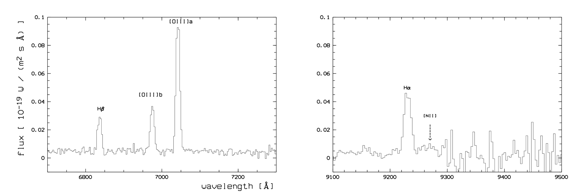
Figure 5: VLT Spectra (mask i) using the 300I grism with FORS2. The “features” observed in the continuum are largely due to residuals from the subtraction of strong OH emission lines. Upper panel: The galaxy 23h-671455 (M${}_{\rm{B}}=-19.0$) at $z\approx 0.4$ shows a ${\rm[N\,II]\,}{\lambda\,6584}$ /${\rm H}{\alpha}$  line ratio of $\sim 0.1$, and lies in the turnaround region of the $\rm R_{23}$  relation. Lower panel: The galaxy 23h-683506 (M${}_{\rm{B}}=-17.3$) at $z\approx 0.4$ shows a ${\rm[N\,II]\,}{\lambda\,6584}$ /${\rm H}{\alpha}$  line ratio $<0.1$, placing this galaxy on the lower branch of the $\rm R_{23}$  relation.

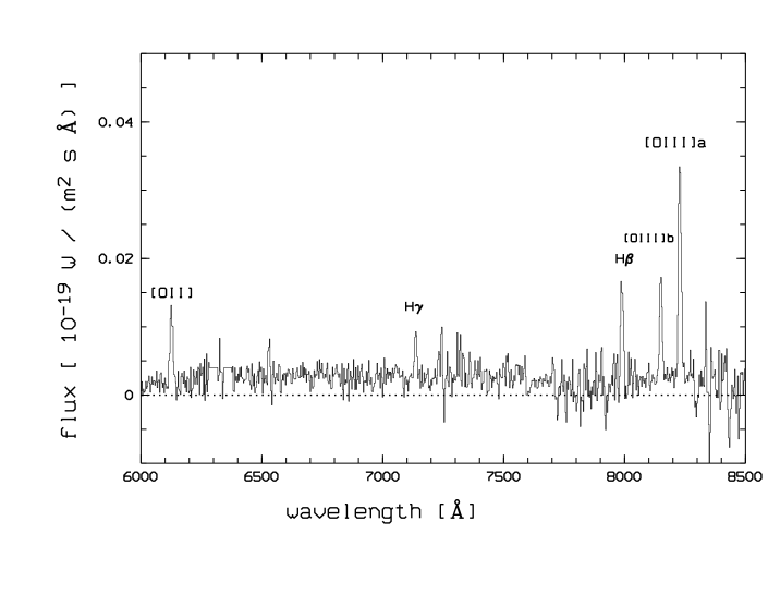
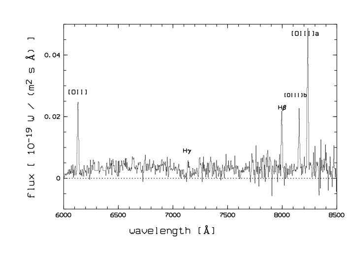
Figure 6: VLT Spectra using the 300I grism with FORS2 of two galaxies at $z\approx 0.64$: 23h-5159 with M${}_{\rm{B}}=-17.5$ (upper panel), and 23h-6512 with M${}_{\rm{B}}=-18.3$ (lower panel). The “features” observed in the continuum are largely due to residuals from the subtraction of strong OH emission lines.

4.3.2 Breaking the $\rm R_{23}$  degeneracy by high ${\rm[O\,III]\,}{\lambda\,5007}$/${\rm[O\,II]\,}{\lambda\,3727}$  flux ratios

From the remaining galaxies without measured ${\rm H}{\alpha}$  and ${\rm[N\,II]\,}{\lambda\,6584}$  (which would require near-infrared spectroscopy for $z\sim 0.64$) three galaxies, 09h-542442, 01h-246610, and 23h-408246, show a high ${\rm[O\,III]\,}{\lambda\,5007}$  to ${\rm[O\,II]\,}{\lambda\,3727}$  flux ratio (greater than five). If we put these galaxies on the upper branch, we would get metallicities of $0.5\,Z_{\hbox{$\odot$}}<Z<1Z_{\hbox{$\odot$}}$. There are no galaxies in the local universe in this high metallicity range which show a such high ${\rm[O\,III]\,}{\lambda\,5007}$/${\rm[O\,II]\,}{\lambda\,3727}$  ratio. Assuming that the physical properties of the interstellar medium are the same in the local universe and at medium redshift, these galaxies cannot have a such high metallicity. Therefore, we have to put them on the lower branch. We used this criterion also for the galaxies 23h-441445 and 23h-552534 (spectra shown in Figure 6).

We exclude the galaxy 01h-628521 oxygen abundance (indicated in Table 2 as (?)) from the following discussion of oxygen abundances, since we cannot be sure on which branch of the $\rm R_{23}$  relation to place it (${\rm[O\,III]\,}{\lambda\,5007}$/${\rm[O\,II]\,}{\lambda\,3727}$ $\sim 1$). Near infrared spectroscopy will be required in order to measure the ${\rm H}{\alpha}$  and ${\rm[N\,II]\,}{\lambda\,6584}$  lines of this galaxy, and to determine on which branch of the $\rm R_{23}$  relation it has to be placed.

4.4 Oxygen abundances

We use the most recent $\rm R_{23}$  formulation by Kobulnicky et al. (kob99 (1999)) of the analytical expressions by McGaugh (mcgaugh (1991)) to determine the oxygen abundances of the emission line galaxies in our sample. These formulae express the oxygen abundance, $12+$log (O/H), in terms of $\rm R_{23}$  and the ionization index ${\rm[O\,III]\,}{\lambda\lambda\,4959,5007}$/${\rm[O\,II]\,}{\lambda\,3727}$. The branch of the $\rm R_{23}$  relation was selected as described in section 4.3. The computed oxygen abundances are shown in Table 2. Additional to the measurement uncertainties of the emission line ratios, an uncertainty of $\sim 0.12$ dex in the oxygen abundance has been assumed, which comes from uncertainties in the photoionization models and ionization parameter corrections for the $\rm R_{23}$  method.

Table 2: Emission line galaxies with unreddened line strengths and computed $\rm R_{23}$  ratios. ^a to ⁱ indicates the mask with which the object was observed (see Table 1). Column Branch indicates if the object lies on the lower (L) or on the upper (U) branch of the O/H versus $\rm R_{23}$  relationship, falls in the turnaround region (T), or if no decision between the upper (U) and lower branch can be made (?). The table is ordered in bins of increasing redshift, at $0.392<z<0.415$, at $0.625<z<0.648$, and $z>0.68$.

#	$z_{spec}$	$M_{B}$	[OIII]/[OII]	[OIII]/${\rm H}{\beta}$	log$\rm R_{23}$	Branch	O/HL	O/$H_{U}$	$12+$log(O/H)
09h-542442f	0.3985	$-$18.1	$11.11\pm 0.79$	$3.03\pm 0.34$	$0.77\pm 0.10$	L	7.64	8.74	$7.64\pm 0.15$
09h-448495f	0.4080	$-$19.2	$1.49\pm 0.11$	$2.38\pm 0.27$	$0.69\pm 0.10$	U	7.81	8.72	$8.72\pm 0.15$
09h-392705f	0.4090	$-$18.4	$0.91\pm 0.06$	$2.94\pm 0.33$	$0.85\pm 0.10$	T	8.16	8.51	$8.34\pm 0.15$
23h-671455i	0.4068	$-$19.0	$0.41\pm 0.07$	$1.96\pm 0.13$	$0.87\pm 0.05$	T	8.30	8.44	$8.37\pm 0.15$
23h-683506i	0.4065	$-$17.3	$1.95\pm 0.61$	$3.05\pm 0.23$	$0.77\pm 0.05$	L	7.90	8.65	$7.90\pm 0.15$
01h-628521d	0.6370	$-$18.7	$1.23\pm 0.07$	$2.30\pm 0.22$	$0.71\pm 0.02$	?	7.86	8.70	?
01h-584247c	0.6358	$-$19.2	$1.59\pm 0.11$	$4.03\pm 0.45$	$0.89\pm 0.10$	T	8.11	8.51	$8.31\pm 0.15$
01h-537252c	0.6372	$-$19.1	$1.25\pm 0.09$	$3.70\pm 0.41$	$0.90\pm 0.10$	T	8.16	8.48	$8.32\pm 0.16$
01h-471561 a	0.6352	$-$18.6	$2.33\pm 0.17$	$3.70\pm 0.41$	$0.84\pm 0.09$	T	7.97	8.60	$8.29\pm 0.31$
01h-246610b	0.6390	$-$17.3	$12.50\pm 1.45$	$4.76\pm 0.53$	$0.83\pm 0.10$	L	7.77	8.67	$7.77\pm 0.15$
01h-177719e	0.6221	$-$18.4	$2.86\pm 0.20$	$5.03\pm 0.56$	$0.95\pm 0.08$	T	8.19	8.46	$8.33\pm 0.14$
23h-441445i	0.6435	$-$17.5	$1.91\pm 0.21$	$1.67\pm 0.16$	$0.53\pm 0.03$	L	7.53	8.85	$7.53\pm 0.15$
23h-558487i	0.6433	$-$18.4	$2.22\pm 0.27$	$4.00\pm 0.45$	$0.86\pm 0.02$	T	8.05	8.55	$8.30\pm 0.15$
23h-552534i	0.6447	$-$18.3	$2.46\pm 0.25$	$2.16\pm 0.20$	$0.59\pm 0.03$	L	7.58	8.82	$7.58\pm 0.15$
23h-408246g	0.6390	$-$18.6	$6.67\pm 0.47$	$5.04\pm 0.56$	$0.85\pm 0.09$	L	7.84	8.65	$7.84\pm 0.15$
23h-431392g	0.6440	$-$19.2	$1.11\pm 0.08$	$3.33\pm 0.37$	$0.87\pm 0.08$	T	8.12	8.57	$8.35\pm 0.23$
23h-385589i	0.6880	$-$18.9	$0.50\pm 0.06$	$2.25\pm 0.25$	$0.88\pm 0.03$	T	8.29	8.44	$8.32\pm 0.30$
23h-645522i	0.8903	$-$19.5	$0.87\pm 0.08$	$2.34\pm 0.23$	$0.77\pm 0.02$	T	8.03	8.61	$8.37\pm 0.15$

5 The metallicity-luminosity relation at medium redshift

Oxygen abundances have been determined for a total number of 15 CADIS emission line galaxies at medium redshift with faint absolute magnitudes ($\rm{M}_{\rm{B}}>-19$). Combining these abundances with published results for galaxies with brighter absolute magnitudes we can study the metallicity-luminosity relation over a large range of luminosities at look-back times of 4.3 Gyrs ($z\approx 0.4$), and 5.9 Gyrs ($z\approx 0.64$). Fig. 7 shows the oxygen abundance as a function of absolute magnitude for two redshift bins, at $z\approx 0.4$, and $z\approx 0.64$, respectively. Additional to the CADIS measurements, oxygen abundances from literature for galaxies in the two redshift bins are shown. It is obvious from the diagrams that only the CADIS emission line sample provides a meaningful sample of $\rm{M}_{\rm{B}}>-19$ galaxies to study the faint absolute magnitudes part of the metallicity-luminosity relation at medium redshift.

Since our number statistics of oxygen abundances at medium redshift are limited, we applied a linear least squares fit to the data. There may be some curvature in this correlation. However, it is not possible to testify such a curvature with our limited sample. For emission line galaxies at $z\approx 0.4$ we find a metallicity-luminosity relation:

$$12+\rm{log}(\rm{O/H})=(4.59\pm 0.91)-(0.199\pm 0.046)M_{B},$$ (6)

with an RMS scatter of 0.219. For emission line galaxies at $z\approx 0.64$ we find a metallicity-luminosity relation:

$$12+\rm{log}(\rm{O/H})=(2.81\pm 0.81)-(0.288\pm 0.042)M_{B},$$ (7)

with an RMS scatter of 0.225. The dotted ($z\sim 0.4$) and dashed-dotted line ($z\sim 0.64$) in Figure 7 are these linear fits showing that a metallicity-luminosity relation exists at medium redshift over a larger luminosity range.

Figure 7: The oxygen abundance as a function of absolute magnitude, for $z\sim 0.4$ (upper panel) and $z\sim 0.64$ (lower panel). The CADIS metallicity measurements are shown as filled squares, open squares show the abundances found by Kobulnicky & Zaritsky (kobzar (1999)) at $z\approx 0.4$, and by Carollo & Lilly (carol (2001)) at $z\approx 0.64$, for more luminous galaxies. Open triangles denote measurements from Kobulnicky et al. (kob03 (2003)). The dotted ($z\sim 0.4$) and dashed-dotted line ($z\sim 0.64$) are linear fits to the data points.

Fig. 8 compares the observed metallicity-luminosity relations at $z=0.4$ and $z=0.64$ (derived in Fig. 7) with the metallicity-luminosity relation for $z=0$ emission line galaxies (Melbourne & Salzer melb (2002)) and the oxygen abundances of luminous galaxies at $z\sim 3.1$ (Kobulnicky & Koo kobko (2000), Pettini et al. pettini (2001)). Moreover, we compare the observed metallicities and luminosities with Pégase2 (Fioc & Rocca-Volmerange fiocrocca (1999)) models.

Figure 8: The metallicity-luminosity relation over a look-back time of $\sim 12$ Gyrs. The solid line shows the luminosity-metallicity relation found by Melbourne & Salzer (melb (2002)) for a large sample of local emission-line galaxies (look back time 0 Gyrs). Also shown are the metallicity-luminosity relations for galaxies in at $z\sim 0.4$ (look back time 4.3 Gyrs), and $z\sim 0.64$ (look back time 5.9 Gyrs) from Fig. 7. The location of bright galaxies at $z\sim 3.1$ is shown as a box encompassing the range of O/H and $\rm{M_{B}}$ derived for these objects (from Fig. 7 in Pettini et al. (pettini (2001)), which takes also into account the metallicities derived by Kobulnicky & Koo (kobko (2000)) for $z\sim 3.1$ objects). The dashed curves and symbols track the chemical and luminous evolution of PÉGASE2 model galaxies with an exponential star formation rate. The galaxies are build by exponentially-decreasing infall of primordial gas (zero metallicity) with infall timescales of 1Gyr and 4Gyrs, respectively. The symbols show galaxies at a look back time of 0, 1, 5, 9, 11 and 12 Gyrs, assuming that the galaxies begin to assemble at a look back time of 13Gyrs.

5.1 Comparison to Pégase2 Models

Pégase2 is a galaxy evolution code which allows to study galaxies by evolutionary synthesis. Here is a discussion of the parameters which were chosen by us:

• $\varphi(IMF)$: The shape of the stellar initial mass function. We adopt the Salpeter value, $\alpha=-2.35$, between 0.1 and 120 $M_{\odot}$ (like Baldry et al. baldry (2002), e.g.).

• $Y$: The chemical yields from nucleosynthesis. We use Woosley & Weaver woosw (1995) B-series models for massive stars.

• $M_{tot}$: The total mass of gas available to form the galaxy. We chose three representative masses of $2\times 10^{10}\,M_{\odot}$, $6\times 10^{10}\,M_{\odot}$, and $2\times 10^{11}\,M_{\odot}$.

• $t_{infall}$: The timescale on which the galaxy is assembled. We assume that galaxies are built by continuous infall of primordial gas (zero metallicity) with an infall rate that declines exponentially, $t_{infall}$, as implemented in Pégase2,

  $$M(t)=M_{tot}\frac{e^{-t/t_{infall}}}{t_{infall}}.$$ (8)

  We chose two representative gas infall timescales of $t_{infall}=1$ Gyr and $t_{infall}=4$ Gyrs.

• $\psi(SFR)$: The form of the star formation rate. We adopt an exponentially decreasing star formation rate, as implemented in Pégase2:

  $$\psi(t)=p2\frac{e^{-t/p1}}{p1}.$$ (9)

• $A_{V}$: Extinction due to dust. An inclination-averaged extinction prescription as implemented in Pégase2 was included, but extinction does not play an important role in the present comparison (it changes the model B magnitudes by only 0.2 mag).

We assume that galaxies begin to form about 1 Gyr after the Big Bang so that local $z=0$ galaxies have ages of about 13 Gyrs (in a 13.5 Gyr old universe). We explored a range of SFR, varying p1 and p2, and the timescale on which the galaxy is assembled, $t_{infall}$. Assuming $p1=t_{infall}$ a high metallicity is reached after less than 1 Gyr, and the metallicity do not change much in the next 12 Gyrs, not reproducing the observed abundances. Models with $p1<t_{infall}$ are unphysical, since SF ceases, although gas is still infalling. Therefore we explored different values of $p1>t_{infall}$. It turned out that, in order to explain the metallicity-luminosity evolution of both luminous galaxies at $z\sim 3$ and galaxies at medium redshift and $z=0$, (representative) models with values of ($t_{infall}=4\,\rm{Gyrs},p1=8$ Gyrs) or ($t_{infall}=1\,\rm{Gyrs},p1=8$ Gyrs), respectively, can reproduce the observed metallicities. The values of $p2$ has been set to $p2=0.2M_{\odot},p2=0.5M_{\odot}$ and $p2=1M_{\odot}$ according to the total mass of a galaxy of $2\times 10^{10}\,M_{\odot}$, $6\times 10^{10}\,M_{\odot}$, and $2\times 10^{11}\,M_{\odot}$, respectively. Thus, only a SFR history with a long exponential timescale ($\sim 8$ Gyrs) can reproduce the observations, but the gas infall has to cease after 1$-$4 Gyrs.

The internal scatter of the metallicity-luminosity relation is relatively well understood in the context of a bursting star formation mode, shown in Mouhcine & Contini (mouhcont (2002)). Therefore, we applied also such a star formation history in our Pégase2 models: we investigated bursting star formation models assuming several bursts of 50 Myrs duration with an inter-burst period of 500 Myrs. The star formation rate is assumed to be proportional to the mass of gas to the power 1.5, with a star formation efficiency $\nu_{s}$ of 3, 1 and 0.5 Gyr^-1, respectively, according to Table 1 in Mouhcine & Contini (mouhcont (2002)) and their equation (3), $\psi(t)=\nu_{\rm{s}}\rm{M}_{\rm{gas}}^{1.5}$ for the starbursting phase. The time for continuous infall of primordial gas, $t_{infall}$, is assumed to be 4 Gyrs. Figure 9 shows, similar to Figure 8, the metallicity predicted by Pégase2 models with these starbursting SFRs for a look backtime of 5 Gyrs and for today, compared to the observed metallicity-luminosity relations. Different from Figure 8 we show here the metallicity-luminosity dependence found putting together all the emission line galaxies at $z\sim 0.4$ and $z\sim 0.64$ (dashed line in Figure 9 labeled as 5 Gyrs ago). This line corresponds to a metallicity-luminosity relation:

$$12+\rm{log}(\rm{O/H})=(3.55\pm 0.60)-(0.251\pm 0.031)M_{B},$$ (10)

with an RMS scatter of 0.227.

Comparison between Figures 8 and 9 shows that the metallicity-luminosity relation at medium redshift is displaced to lower abundances and higher luminosities compared to today. This can be explained independent of the assumption of a starbursting star formation history in the Pégase2 models or of an exponentially decreasing star formation rate. The shift we see in the Figures 8 and 9 is comparable to the internal scatter of the metallicity-luminosity relation today and at medium redshift. However, our emission line sample is not biased compared to the Melbourne and Salzer local sample. Therefore we think that the shift in our mean relation reflects a true shift, in the sense that the metallicity of galaxies increases and their luminosity decreases between $z\sim 0.7$ and $z\sim 0$.

Figure 9: The metallicity-luminosity relation, similar to Figure 8, but for starbursts models of Mouhcine & Contini (mouhcont (2002)). Moreover, the dashed line labeled as 5 Gyrs look back time is the metallicity-luminosity relation found puting together the metallicities of all emission line galaxies at $z\sim 0.4$ and $z\sim 0.64$.

5.2 Discussion

Galaxies over a large range of absolute magnitude ($-17\la\rm{M}_{\rm{B}}\la-22$) show an evolution of the metallicity-luminosity at $z\sim 0.4$ and $z\sim 0.64$ compared to $z=0$. Comparison with Pégase2 models shows a possible scenario in which galaxies at medium redshift have faded by $\sim 0.5\,\rm{mag}$ (galaxies with lower luminosities in Fig.8) up to $\sim 0.9\,\rm{mag}$ (galaxies with higher luminosities in Fig.8) in $\sim 6$ Gyrs due to decreasing levels of star formation, and their metallicity has increased by a factor of $\sim 0.3\,\rm{dex}$.

The luminosity evolution of $\Delta\rm{M_{B}}=0.5-0.9$ mag between $z=0$ and $z=0.64$ (5.9 Gyr ago) is consistent with the observational results of the COMBO-17 survey (Wolf et al. wolf (2003), their Fig.17): They find that $\rm{M^{*}_{B}}$ of starburst galaxies decreases by $\sim 0.5$ mag between $z=0.7$ and $z=0.3$.

Fig. 8 and 9 show an increase of metallicity by a factor of $\sim 2$ for galaxies in the local universe compared to medium redshift. The metallicity evolution is consistent with models of Somerville & Primack (somerv (1999)) and Pei et al. (pei (1999)), who predict a change in the star-forming metallicity with redshift of 0.2 dex, and 0.3 dex, respectively, over the last half of the age of the universe (see also Fig.  18 in Lilly et al. lilly03 (2003)). Our result is also consistent with the finding of Lilly et al. (lilly03 (2003)): Based on estimates of the oxygen abundance in a sample of 66 CFRS galaxies at $0.47<z<0.92$ they argue that luminous low metallicity galaxies at medium redshift, which have normal mass-to-light ratios and relatively large sizes, will evolve to higher metallicity galaxies of similar absolute magnitudes rather than to fainter low metallicity galaxies.

Acknowledgements

We are grateful to the anonymous referee for his/her suggestions that have improved the paper. We thank A. Aguirre and M. Alises from the Calar Alto Observatory for carring out CADIS observations in service mode, and we thank Francisco Prada for obtaining TNG observing time in the Spanish panel. We also thank Eric Bell, Ignacio Ferreras, Alexei Kniazev, Henry Lee and Simon Lilly for valuable discussions.

References

- (1) Baldry, I. K., Glazebrook, K., Baugh, C. M. et al. 2002, ApJ, 569, 582
- (2) Brocklehurst M. 1971 MNRAS, 153, 471
- (3) Carollo C. M. & Lilly S. J. 2001, ApJ, 548, 153
- (4) Cohen, J.G. 2002, ApJ, 567, 672
- (5) Contini T., Treyer M. A., Sullivan M. & Ellis R. S. 2002, MNRAS, 330, 75
- (6) Denicolo G., Terlevich R. and Terlevich E. 2002, MNRAS, 330, 69
- (7) Fioc, M. & Rocca-Volmerange, B., 1999, astro-ph/9912179
- (8) Garnett D. R., Shields G. A., Skillman E. D., Sagan S. P. & Dufour R. J. 1997, ApJ, 489, 63
- (9) Grevesse, N., Noels, A., Sauval, A. J. 1996. Standard Abundances; in S. S. Holt and G. Sonneborn (Eds.), Cosmic Abundances: Proceedings of the 6th annual October Astrophysics Conference, Volume 99 of A.S.P. Conference Series, p.117. San Francisco: Astron. Soc. of the Pacific
- (10) Hammer F., Gruel N., Thuan T. X. and Infante L. 2001, ApJ, 550, 570
- (11) Hamuy, M., Walker, A. R., Suntzeff, N. B. et al. 1992, PASP 104, 533
- (12) Hamuy, M, Suntzeff, N. B., Heathcote, S. R. et al. 1994, PASP 106, 566
- (13) Hippelein, H., Maier, C., Meisenheimer, K. et al. 2003, A&A, 402, 65
- (14) Horne K. 1986, PASP, 98, 609
- (15) Hunter D. A. & Hoffman L. 1999, AJ, 117, 2789
- (16) Izotov Y. I., Thuan Trinh T. & Lipovetsky V. A. 1994, ApJ, 435, 647
- (17) Kauffmann, G. 1996 MNRAS, 281, 475
- (18) Kennicut, R.C.Jr. 1998, ApJ, 498, 541
- (19) Kniazev, A.Y., Pustilnik, S.A., Grebel, E.K. et al. 2004, Strong Emission Line HII Galaxies in the Sloan Digital Sky Survey. I. Catalog of DR1 Objects with Oxygen Abundances from Te Measurements, submitted to ApJS
- (20) Kobulnicky, H. A., Wilmer C. N. A., Weiner, B. J. et al. 2003, ApJ, 599, 1006
- (21) Kobulnicky, H. A. & Koo, D. C. 2000, ApJ, 545, 712
- (22) Kobulnicky, H. A., Kennicutt R. C. Jr. & Pizagno J. L. 1999, ApJ, 514, 544
- (23) Kobulnicky, H. A. & Zaritsky D. 1999, ApJ, 511, 118
- (24) Lilly, S.J, Carollo, C.M. & Stockton, A.N. 2003, ApJ, 597, 730
- (25) MacLow, M. & Ferrara, A. 1999, ApJ, 513, 142
- (26) McCall L. M., Rybski P. M. & Shields G. A. 1985, ApJS, 57, 1
- (27) McGaugh, Stacy 1991, ApJ, 380, 140
- (28) Maier, C., Meisenheimer, K., Thommes, E. et al. 2003, A&A, 402, 79
- (29) Meisenheimer, K., Beckwith, S., Fockenbrock, H. et al. 1998, in The Young Universe: Galaxy Formation and Evolution at Intermediate and High Redshift. Edited by S. D’Odorico, A. Fontana, and E. Giallongo. ASP Conference Series, Vol. 146, p.134
- (30) Meisenheimer, K. et al. 2004, The Calar Alto Deep Imaging Survey: Concept, Data Analysis and Calibration, in preparation
- (31) Melbourne, J. & Salzer, J. J. 2002, AJ, 123, 2302
- (32) Mouhcine, M. & Contini, T. 2002, A&A, 389, 106
- (33) Oke, J. B. 1990, AJ, 99, 1621
- (34) Osterbrock, D.E. 1989, Astrophysics of Gaseous Nebulae and Active Galactic Nuclei (Mill Valley: University Science Books)
- (35) Pagel, B. E. J., Edmunds, M. G., Blackwell, D. E. et al. 1979, MNRAS, 189, 95
- (36) Pagel., B. E. J., Nucleosynthesis and chemical evolution of galaxies, Cambridge : Cambridge University Press, 1997
- (37) Pei, Y.C., Fall, M., Hauser, M.G. 1999 ApJ, 522, 604
- (38) Pettini, M., Shapley, A. E., Steidel, C. C. 2001, AJ, 554, 981
- (39) Seaton, M. J. MNRAS 1979, 187, 73
- (40) Shields, G. A. ARAA, 1990, 28, 525
- (41) Somerville, R. S., & Primack, J. R. 1999, MNRAS, 310, 1087
- (42) Stasinska, G. & Leitherer, C. 1996, ApJS, 107, 661
- (43) Richer, M. G. & McCall, M. L. 1995, ApJ, 445, 642
- (44) Skillman, E. D., Kennicutt, R C. & Hodge, P.W. 1989, ApJ, 347, 875
- (45) Skillman, E. D. & Kennicutt, R C. Jr. 1993, ApJ, 411, 655
- (46) Wolf, C., Meisenheimer, K., Rix, H.-W. et al 2003, A&A, 401, 73
- (47) Woosley, S. E. & Weaver, T. A. 1995, ApJS, 101, 181
- (48) Whitford, A. E., 1958, AJ, 63, 201
- (49) Zaritsky, D., Kennicutt, R.C. & Huchra, J.P. 1994, ApJ, 420, 87