Variations of the

Fine Structure Constant

in Space and Time

David Fonseca Mota
Corpus Christi College

Dissertation submitted for the degree of Doctor of Philosophy
Department of Applied Mathematics and Theoretical Physics
University of Cambridge
September 2003

A descoberta dessa impossibilidade,
a de sermos já no caminhar e só no caminhar o sermos;
não podendo ser de outra maneira,
é a possibilidade de criar o nosso modo de caminhar
– Ernesto Mota –

This thesis is dedicated to my parents:
Irene Fonseca (Mãezitas) and Joaquim Mota (Paizolas)

DECLARATION

The research presented in this thesis was performed in the Department of Applied Mathematics and Theoretical Physics at the University of Cambridge between October 1999 and August 2003. This dissertation is the result of my own work, except as stated below or where explicit reference is made to the results of others. Chapters 2, 3, 4 and 5 of this thesis are respectively based on the papers (Refs. [1, 2, 3, 4]):

• J. D. Barrow and D. F. Mota, “Qualitative analysis of universes with varying alpha”, Class. Quant. Grav.  19, 6197 (2002) [arXiv:gr-qc/0207012].

• J. D. Barrow and D. F. Mota, “Gauge-invariant perturbations of varying-alpha cosmologies”, Class. Quant. Grav.  20, 2045 (2003) [arXiv:gr-qc/0212032].

• D. F. Mota and J. D. Barrow, “Varying Alpha in a More Realistic Universe”, Submitted to Phys. Lett. B, [arXiv:astro-ph/0306047]

• D. F. Mota and J. D. Barrow, “Local and Global Variations of The Fine Structure Constant”, Submitted to Mon. Not. Roy. Astron. Soc. , [arXiv:astro-ph/0309273]

Much of the work of chapters 2,  3,  4 and 5 was a result of a close collaborative effort with my supervisor John D. Barrow. In chapter 2, my supervisor has set up the approximation method, the validity of the approximation and the linearisation of the instability. He has also found the exact solution in the $n>2/3$ case and has performed the stability analysis of the $n=2/3$ asymptote. In chapters 3,  4 and 5, my supervisor has contributed to the interpretation, discussion and clarification of the results.

This dissertation is not substantially the same as any that I have submitted, or am submitting, for a degree, diploma or other qualification at any other university.

Signed: …………………………………             Dated: ………………………………….

ACKNOWLEDGEMENTS

I would like to thank my supervisor John D. Barrow for his constant advice, encouragement, enthusiasm and support over my years here in Cambridge.

During the course of this work I have had helpful discussions with many people for which I am very grateful, including Carsten van de Bruck, Martin Bucher, João Lopes Dias, Yves Gaspar, Kaviland Moodley, Michael Murphy, Fernando Quevedo and Constantinos Skordis.

I would like to thank Pedro Ferreira and Joseph Silk for hospitality at the Oxford University Physics Department during the time when part of this thesis was written.

I also would like to thank Orfeu Bertolami for his encouragement and support to apply to Cambridge while still an undergraduate student in Lisbon.

For the financial support, I would like to thank Fundação para a Ciência e a Tecnologia, through the research grant BD/15981/98 and Fundação Calouste Gulbênkian, through the research grant Proc.50096.

On a personal note I would like to thank the unforgettable and unique friendship of Milind, John, Pearson and Al during all these years in Cambridge. Many others have contribute to my enjoyable stay in Cambridge they are Andre, Caroline, Jose, Khaled, Maria João, Miguel, Nidhi, Nuno, Pedro, Saghir, Shaun and Toto.

Although not living in Cambridge, I would like to thank Marisa and my ’new family’ Adriano Couto, Maria de Lurdes, Marie-Thérèse and Marlène for their friendship. I also would like to thank my grandmother, Maria da Conceição, and my aunt, Zeza, to whom I will be always grateful for taking care of me, and for all their love, since I was a baby.

In a very special way, I would like to thank my parents, for their love and support over all these years, of which, as far as I can remember, have always encourage me to “learn more” and to “widen my horizons”.

To my brother, Ernesto, any word of gratitude would be too small, I may only say: Thank you for existing.

Finally it is an honour to thank my wife and soul-mate Elisabeth for her understanding and patience throughout the process of writing the thesis. Most specially, thank you for all your love and encouragement when I most need it.

Variations of the Fine Structure Constant in Space and Time
David Fonseca Mota
Summary

This thesis describes a detailed investigation of the effects of matter inhomogeneities on the cosmological evolution of the fine structure constant.

In chapter 1, we briefly describe the observational and theoretical motivations to this work. and we review the standard cosmological model. We also review the Bekenstein-Sandvik-Barrow-Magueijo (BSBM) theory for a varying fine structure constant, $\alpha$.

Assuming a Friedmann universe which evolves with a power-law scale factor, $a=t^{n}$, in chapter 2, we analyse the phase space of the system of equations that describes a time-varying $\alpha$, in a homogeneous and isotropic background universe. We classify all the possible behaviours of $\alpha(t)$ in ever-expanding universes with different $n$ and find exact solutions for $\alpha(t)$. In general, $\alpha$ will be a non-decreasing function of time that increases logarithmically in time during a period when the expansion is dust-dominated ($n=2/3$), but becomes constant when $n>2/3$. $\alpha$ tends rapidly to a constant when the expansion scale factor increases exponentially. A general set of conditions is established for $\alpha$ to become asymptotically constant at late times in an expanding universe.

In chapter 3, using a gauge-invariant formalism, we derive and solve the linearly perturbed Einstein cosmological equations for the BSBM theory. We calculate the time evolution of inhomogeneous perturbations of the fine structure constant, $\frac{\delta\alpha}{\alpha}$ on small and large scales with respect to the Hubble radius. In a radiation-dominated universe small inhomogeneities in $\alpha$ decay on large scales but on scales smaller than the Hubble radius they undergo stable oscillations. In a dust-dominated universe, small inhomogeneous perturbations in $\alpha$ approach a constant on large scales and on small scales they grow as $t^{2/3}$, and $\frac{\delta\alpha}{\alpha}$ tracks $\frac{\delta\rho_{m}}{\rho_{m}}$ . If the expansion accelerates, as in the case of a $\Lambda$ or quintessence-dominated phase, inhomogeneities in $\alpha$ decay on both large and small scales. The amplitude of perturbations in $\alpha$ are much smaller than that of matter or radiation perturbations. We also present a numerical study of the non-linear evolution of spherical inhomogeneities in radiation and dust universes by means of a comparison between the evolution of flat and closed Friedmann models with time-varying $\alpha.$Various limitations of these simple models are also discussed.

Chapter 4 is dedicated to the effects of non-linear structure formation in the evolution of $\alpha$. We study the space-time evolution of the fine structure constant inside evolving spherical overdensities in a $\Lambda$ Cold Dark Matter ($CDM$) Friedmann universe, using the spherical infall model. We show that its value inside virialised regions will be significantly larger than in the low-density background universe. The consideration of the inhomogeneous evolution of the universe is therefore essential for a correct comparison of extragalactic and solar system limits on, and observations of, possible time variation of $\alpha$ and other constants. Time variation of $\alpha$ in the cosmological background can give rise to no locally observable variations inside virialised overdensities like the one in which we live, explaining the discrepancy between astrophysical and geochemical observations.

In chapter 5, using the BSBM varying-alpha theory, and the spherical collapse model for cosmological structure formation, we study the effects of the dark-energy equation of state and the coupling of $\alpha$ to the matter fields on the space and time evolution of $\alpha$. We compare its evolution inside virialised overdensities with that in the cosmological background, using the standard ($\Lambda=0$) $CDM$ model of structure formation and the dark-energy modification, $wCDM$. We find that, independently of the model of structure formation one considers, there is always a difference between the value of alpha in an overdensity and in the background. In a $SCDM$ model, this difference is the same, independent of the virialisation redshift of the overdense region. In the case of a $wCDM$ model, especially at low redshifts, the difference depends on the time when virialisation occurs and the equation of state of the dark energy. At high redshifts, when the $wCDM$ model becomes asymptotically equivalent to the $SCDM$ one, the difference is constant. At low redshifts, when dark energy starts to dominate the cosmological expansion, the difference between $\alpha$ in a cluster and in the background grows.

The last chapter contains a summary of the results obtained in the thesis and a discussion of some open problems that require further investigation.

Chapter 1 Introduction

… contudo fazemos da nossa angustia,
desta quietude irriquieta que nos atormenta a alma,
as mil e uma perguntas sem resposta…
– Ernesto Mota –

1.1 Constants of Nature

Once upon a time, humankind started to describe the universe we live in using mathematics. When a mathematical formalism is proposed in order to describe the different phenomena that occur in our universe, a theory in physics is set. Any theory which claims to explain a set of events in nature has to be confronted with the empirical observations. Hence, having the formal structure of a given physical theory, there is the need to quantify it in order to test it. The quantification of a given physical model consist in the introduction of numbers. But this raises a question: How shall we choose these numbers and to which quantities shall we attribute them? Theories in physics have several free parameters of which value cannot be calculated or deduced from its formal structure. These free parameters are the fundamental constants of the theory. We need to attribute a value to these quantities, and the value is chosen in order to match the quantitative predictions of the theory with the observations and experiments performed. Why are these quantities fundamental? Because their values cannot be calculated, only measured. Why constant? Because every experiment yields the same value independently of time, position, temperature, pressure, etc.

But not all the constants in physics are fundamental. If one conducts an experiment with greater precision and/or in an environment more extreme than previously considered, one might observe variations of the constants. This may precipitate physicists to search for a more basic theory which explains the origin and the value of the (then non-fundamental and variable) constant. The status of a constant depends then on the considered theory and on the observer measuring them, that is, on whether this observer belongs to the world of low-energy quasi-particles or to the high energies one. For example, the density of a given material was once regarded as constant, but was later found by experimenters to vary with temperature and pressure.

1.1.1 Why study variations of the fundamental constants?

By definition, the constants of nature are quantities which have no dependence on other measured parameters, it is not surprising that despite the enormous advances in particle physics we still have no idea why the constants of nature take the values they do. This might be something we will never be able to answer, but we have learnt from the past, that what we call today a constant might not be so in the future.

The hypothesis of the constancy of the fundamental constants plays an important role in astronomy and cosmology where the redshift measures the look-back time. Ignoring the possibility of varying constants could lead to a distorted view of our universe and if such variations are established corrections should be applied. It is thus important to investigate that possibility, especially as the measurements become more precise.

The study of the variations of the constants of nature also offers a new link between astrophysics, cosmology and high-energy physics complementary to early universe cosmology. In particular, the observation of the variability of the fundamental constants constitutes one of the few ways to test directly the existence of extra-dimensions and to test high energy physics models.

From all the possible fundamental constants of nature we will focus on the so called fine structure constant, $\alpha$. The fine structure constant is also regarded as the coupling constant of the electromagnetic interactions. The fine structure constant can be derived from other constants as follows [6]:

$$\alpha=\frac{e^{2}}{4\pi\epsilon_{0}\hbar c}$$ (1.1.1)

where $c$ is the speed of light in vacuum, $\hbar\equiv h/2\pi$ is the reduced Planck constant, $e$ is the electron charge magnitude and $\epsilon_{0}$ is the permitivity of free space. The value of $\alpha$ measured today on earth is $\alpha_{0}\approx 1/137.035$ [6].

In this thesis we will study the theoretical possibilities of time and spatial variations of the fine structure constant along the history of the universe.

Time variations of $\alpha$ can be measured using the ’time shift density parameter’:

$$\frac{\Delta\alpha}{\alpha}\equiv\frac{\alpha(z)-\alpha_{0}}{\alpha_{0}}$$ (1.1.2)

where $\alpha(z)$ is the value of the fine structure constant at a redshift $z$. Similarly, spatial variations of $\alpha$ can be studied using the ’spatial shift density parameter’:

$$\frac{\delta\alpha}{\alpha}\equiv\frac{\alpha_{x_{1}}(z)-\alpha_{x_{2}}(z)}{\alpha_{x_{2}}(z)}$$ (1.1.3)

where $\alpha_{x_{1,2}}$ is the value of the fine structure constant in a two different regions in the universe, for instance $x_{1}$ and $x_{2}$ can represent two different galaxies.

But why shall we look at possible variations of the fine structure constant? The next two sections describe both observational and theoretical motivations for this work.

1.2 Observations and Constraints on Variations of the Fine Structure Constant

Many methods were used to observe possible variations of the fine structure constant [7]. A general conclusion of those experiments and observations, is that there is no variation of $\alpha$, or at least the results are consistent with the hypothesis of a null variation. If there are any time or spatial variations of $\alpha$, these will be very small. Hence, up to nowadays, we basically have upper limits that constraint variations of the fine structure constant. Nevertheless, there is at least one observation which explicitly gives a non-null result for variations of $\alpha$. As we will see, this observation has a very unique feature: It has observed variations in the fine structure constant in a redshift range of $z=0.5-3.5$.

When taking conclusions from experiments and observations on variations (or none) of the constants of nature we should always bear in mind that those measurements are set on a given time-scale. Hence we need to be very careful when extrapolating those results into an absolute conclusion. For instance, in the case of the fine structure constant, one expect to be able to constrain a relative variation of $\alpha$ in a time scale of $10^{9}$ years ($z\approx 0.3$) using geochemical constraints [8]; $10^{9}-10^{10}$ years ($z\approx 3$) using astrophysical (quasars) methods [5]; $10^{10}$ years ($z\approx 1000$) using cosmological methods (Cosmic Microwave Background Radiation) [9]; and $1-12$ months using laboratory methods [10]. It is then not a straight forward task to interpret and take absolute conclusions from most of the observations performed until today. For example, if we observe no time variations of $\alpha$ using geochemical methods, we can only conclude that the fine structure constant did not vary from a redshift $z=0.3$ up to today.

Another common feature to the observational and experimental results is the presence of degeneracies. Usually, there are other parameters in the model, used to study the physical phenomenon, that may influence the results. Due to that, the conclusions taken are then based on some assumptions, which usually lead to an extra error bar besides the systematic experimental errors. The problem of the degeneracies is not an easy one, since such analyses are also dependent on our understanding of the fundamental interactions [11, 12]. For instance, grand unifying theories predict that all the constants should vary simultaneously. One needs to further study the systematic errors of the observations and to propose and realise new experiments which are less model dependent [13, 14].

In this section, we shall not attempt to give a full review, deferring the reader to [7] and the references therein.

1.2.1 Geochemical constraints

All the geological studies are on time scales of order of the age of the Earth, meaning that constraint variations of the fine structure constant in a range of redshifts of $z\approx 0.1-0.15$, depending on the values of the cosmological parameters.

Atomic clocks are one of the principal methods we have to measure possible variations of the fine structure constant on Earth. The latest constraint on possible variations of $\alpha$, using atomic clocks, is [15]:

$$\left|\frac{\dot{\alpha}}{\alpha}\right|<4.2\times 10^{-15}~{}{\rm yr}^{-1}\,.$$ (1.2.1)

Notice that, although the constraint is very tight, it is only valid for a very short period of time. Usually a few months, the time the experience lasted.

One of the oldest observations, with non-null results, looking for variations of the fine structure constant came from the analysis of the Oklo phenomenon - a natural nuclear fission reactor which operated in Gabon, Africa, at approximately $1.8$ billion years ago [16, 17, 18, 19]. The first analysis were done by Shlyakhter [20] and an upper limit on time variations of $\alpha$ resulted to be: $\Delta\alpha/\alpha<10^{-7}$ over a period of $1.8$ billion years. However that study provided two possible results:

$$\frac{\dot{\alpha}}{\alpha}=\left(-0.2\pm 0.8\right)\times 10^{-17}\qquad\text{per year}$$ (1.2.2)

$$\frac{\dot{\alpha}}{\alpha}=\left(4.9\pm 0.4\right)\times 10^{-17}\qquad\text{per year}$$ (1.2.3)

which come from two possible physical branches [16, 20, 21]. Note that only the first solution is consistent with a null variation of the fine structure constant, whereas the other implies a higher value of $\alpha$ in the past.

Recently many others analysis were performed using the Oklo phenomenon [8, 22, 21]. Up to today, the tighter constraint using new samples from the Oklo reactor is:

$$\frac{\Delta\alpha}{\alpha}=\left(-0.04\pm 0.15\right)\times 10^{-7}$$ (1.2.4)

These limits should be considered with care, since in general there are considerable uncertainties regarding the complicated Oklo environment and any limits on $\alpha$ derived from it can be weakened by allowing other interaction strengths and mass ratios to vary in time as well [23, 21].

Constraints at slightly higher redshifts

Another geochemical process, which is sensitive to changes in $\alpha$, is the $\beta$-decay rate of ${}^{187}Re$ [24]. Updating the work of Dyson [25, 26], Olive et al. [21] claim that, improved measurements of the ${}^{187}Re$ $\beta-$decay rate (derived from meteoritic ${}^{187}Re/^{187}Os$ abundances ratios), imply $|\Delta\alpha/\alpha|<3\times 10^{-7}$ over the $4.65$ Gyr history of the solar system ($z\approx 0.45$). However, Uzan [7] notes that the above result assumes that variations of the $\beta$-decay rate depend entirely on variations of $\alpha$ and not on possible variations of the weak coupling constant, see also [27]. Very recently, Olive et al. [28], have rederived this constraint, in models where all gauge and Yukawa couplings vary independently, as would be expected in grand unification theories. The new constraint is $|\Delta\alpha/\alpha|<(-8\pm 8)\times 10^{-7}$. In spite of the potential problems of these experiments, the study of this phenomenon is quite important. It provides constraints to variations of $\alpha$ at slightly higher redshift than the usual geochemical constraints, and at the same time, it give us a hint on the possible evolution of the fine structure constant inside our local system of gravity.

1.2.2 Astrophysical observations

Astrophysical observation are probably one of the most important types of experiments which can be performed in order to study the possibility of variations of the fine structure constant in cosmological scales.

Observing the quasar absorption spectra give us information about the atomic levels at their position and time of emissions. It is usually assumed, in those observations, that all transitions have the same $\alpha$ dependence. So any variation of the fine structure constant will affect all the wave lengths by the same factor. Another assumption is the independence of this uniform shift of the spectra from the Doppler effect due to the motion of the source or to the gravitational field where it sits. The idea is to compare different absorption lines from different species to extract information about different combinations of the constants at the time of emission and then to compare them with the laboratory values (see [29] for a detailed description). A quite surprising result was obtained from these observations: an explicit time variation of the fine structure constant was found. The value of $\alpha$, in a redshift range of $z=0.5-3.5$, was smaller than the standard value on earth $\alpha_{0}$ [5, 30, 31, 32, 33] (see however [34] for another interpretation of the results). The latest value for the time shift parameter of the fine structure constant is [35]:

$$\frac{\Delta\alpha}{\alpha}=-0.543\pm 0.116\times 10^{-5}$$ (1.2.5)

for a redshift range of $z=0.5-3.5$.

Many other astrophysical observations were performed [36, 37, 38, 39, 40, 41], but none of them has explicitly indicate the existence of variations of the fine structure constant, that is, they are just upper bounds. This show us how relevant and important are the series of results obtained from the quasar absorption spectra. Such a non-zero detection, if confirmed, would bring tremendous implications on our understanding of physics, for instance, it would be interesting to investigate if such a variation is compatible with the test of the universality of free fall [42].

Note that, a feature of the results from the quasar absorption spectra, is that they are ’incompatible’ with the geochemical observations if the variation of $\alpha$ is linear with time. If both the geochemical and the quasar’s absorption spectra observations are confirmed, then the theoretical models proposed to explain variations of $\alpha$ will need to explain the reason for such a discrepancy between astrophysical observations and geochemical ones. In particular, the constraint of $\Delta\alpha/\alpha\leq 3\times 10^{-7}$ at redshift $z=0.45$, coming from the $\beta$-decay experiments, is very difficult to be compatible with an explicit variation of the fine structure constant of $\Delta\alpha/\alpha\approx 5\times 10^{-6}$ at $z=0.5$, coming from the quasar’s absorption spectra.

1.2.3 Early universe constraints

Cosmic Microwave Background Radiation

Time or spatial variations of the fine structure constant affect the power-spectrum of the Cosmic Microwave Background Radiation (CMBR) anisotropies [43, 44]. This is due to the fact that a different value of $\alpha$ would affect the biding energy of hydrogen, the Thompson scattering cross section and the recombination rates. A smaller value of $\alpha$ would postpone the recombination of electrons and protons, i.e., the last scattering would occur at a lower redshift. It would also alter the baryon-to-photon ratio at last-scattering, leading to changes in both the amplitudes and positions of features in the power spectrum. The strongest current constraints at $z\approx 1000$ from the CMBR power spectrum are at the $\Delta\alpha/\alpha\approx 10^{-2}$ level if one considers the uncertainties in, and degeneracies with, the usual cosmological parameters (for instance $\Omega_{m},\Omega_{\Lambda}$, etc) [9, 45, 46, 47, 48, 49]. However, note there is a critical degeneracy between variations of $\alpha$ and the electron mass $m_{e}$ [50, 51], since the relativistic-quantum corrections of the electron mass depend on the strength of the electromagnetic interaction and consequently on $\alpha$. This degeneracy dramatically weakens the current constraints.

Big Bang Nucleosynthesis

The theory of Big Bang Nucleosynthesis (BBN) is one of the corner-stones of the hot Big Bang cosmology, successfully explaining the abundances of the light elements, $D$, ${}^{3}He$, ${}^{4}He$ and ${}^{7}Li$. Assuming a simple scaling between the value of $\alpha$ and the proton-neutron mass difference a limit can be placed on $\Delta\alpha/\alpha$ [52]. A similar method can be used considering simultaneous variations of the weak, strong and electromagnetic couplings on BBN [53]. However, in general, estimates based on BBN abundances of ${}^{4}He$ suffer from the crucial uncertainty of electromagnetic contribution to the proton-neutron mass difference. Much weaker limits are possible if attention is restricted to the nuclear interaction effects on the nucleosynthesis of $D$, ${}^{3}He$ and ${}^{7}Li$ [54, 55]. Given the present observational uncertainties in the light element abundances, the most conservative limits are $\Delta\alpha/\alpha=(3\pm 7)\times 10^{-2}$.

1.3 Theoretical Motivations

In the previous section we have described the empirical motivations to study variations of the fine structure constant. In reality, they were not very convincing, since most of the results are basically upper bounds to variations of $\alpha$ and the only explicit results, that claimed a lower value of $\alpha$ in the past, was presented by a sole group of collaborators in a series of experiments [35, 5, 30, 31, 32, 33].

The situation is completely different from the theoretical point of view. We will see that there are several important reasons why we should seriously take into account the possibility of a varying-$\alpha$. Most of them come from theoretical models which try to give a more complete description of the universe.

These theories have strong observational predictions, for instance, in the case of a time-varying $\alpha$, they allow us to evaluate the effects of a varying $\alpha$ on free fall which leads to potentially observable violations of the weak equivalence principle [56, 57, 58, 42]. They also allow us to investigate whether or not other cosmological observations like the Cosmic Microwave Background Radiation are consistent with the variations of $\alpha$ to fit the quasar observations [46, 9, 51].

Once again we shall not attempt to give a full review here, deferring the reader to [7] and [59] for a more thorough discussion.

1.3.1 Multi-dimensional theoretical models

There are very strong theoretical motivations to study time and spatial variations of the fine structure constant. The reasons come essentially from novel theories which claim to be more ’fundamental’ and so are candidates to be the ’Theory of Everything’. The best candidates for unification of the forces of nature, in a single unified theory of quantum gravity, only seem to exist in finite form if there are more dimensions of space than the common four that we are familiar with. This means that the true constants of nature are defined in a higher dimensional world and the constants we observe are merely effective values, that is, they are a four-dimensional projection of the real fundamental constants. So the coupling constants we observe and measure may not be fundamental and so do not need to be constant.

Since we do not observe any other dimensions than the common four, there is a strong indication that, if those extra-dimensions exist, they are indeed very small. A general feature of the multi-dimensional theories, is that the size of the extra-dimensions is associated to a scalar field. This field is a dynamical quantity, which has the desired property of making the extra-dimensions small and stable (in the sense that their size will not change). The reason why we desire the stability of the extra-dimensions, is related to the fact that in most of the cases that scalar field will be coupled to the matter fields. Any time or spacial variations of this field will then be ’seen’ as a variation of the interactions’ coupling constants. Up to nowadays, no mechanisms of stabilising the scalar field, was found. Hence, until this mechanism is to be found, a common feature of the multi-dimensional theories is the existence of slow changes in the scale of the extra-dimensions which would be revealed by measurable changes in our four-dimensional “constants”.

Multi-dimensional theories also predict relations between different constants, due to relations between the coupling of dilaton type fields and matter, see for instance [60, 61, 62, 63] for more complex effects then just the variation of the coupling constants.

One of the earliest attempts to create a single unified theory was presented by Kaluza [64] and Klein [65]. They considered a five-dimensional model with the aim to unify electromagnetism and gravity (for a review see [66]). The fifth dimension is compactified in order to turn it small. The compactification results into a coupling between the scalar field, which is related to the radius of the fifth dimension, and the matter fields. Variations of the scalar field will be reflected as variations of all the coupling constants. Various functional forms for monotonic time variations have been derived where usually the four-dimensional gauge couplings vary as the inverse square of the mean scale of the extra dimension (for instance see [60, 67, 68]). Non-monotonic variations of $\alpha$ with time where analysed in [69] and the requirements for a self-consistent relations, if there are simultaneous variations of the different coupling constants, were discussed. Other five-dimensional theories, based on the so called Brane-World models, were also used to study variations of the fine structure constant. See for instance [7, 59, 70, 71] and references therein.

A much more recent and popular candidate to a theory of unification is string theory. Superstrings theories offer a theoretical framework to discuss the value of the fundamental constants since they become expectation values of some fields [7]. One of the definitive predictions of superstring theories is the existence of a scalar field, the dilaton, that couples directly to matter [72] and whose vacuum expectation value determines the string coupling constant [73]. The four-dimensional couplings are determined in terms of a string scale and various dynamical fields, for instance, the dilaton and the volume of compact space. Due to the coupling between the dilaton and all the matter fields, we expect the following effects: a scalar mixture of a scalar component inducing deviations from general relativity, a variation of the coupling constants, and a violation of the weak equivalence principle [7]. Various string theories will exhibit different variations of the effective couplings; in particular, the cosmological evolution of the fine structure constant will depend on the form of the coupling between the dilaton and the matter fields which interact electromagnetically. The undefined structure of the coupling gave origin to many low energy models and approaches to study time and spatial variations of the fundamental constants and its relation to the extra-dimension radius (see for instance [52, 74, 75, 76, 77]). In [58] it was shown that cosmological variations of $\alpha$ may proceed at different rates at different points in space-time (see also [78, 79, 80]). This mean that variations of the fine structure constant may not only be in time but in space as well.

1.3.2 The Bekenstein model for varying-$\alpha$

Independently of any extra-dimensional model, Bekenstein [81, 82, 83] formulated a framework to incorporate a varying fine structure constant. Working in units in which $\hbar$ and $c$ are constants, he adopted a classical description of the electromagnetic field and made a set of assumptions to obtain a reasonable modification of Maxwell equations to take into account the effect of the variation of the elementary charge, $e$. His eight postulates are: (i) For a constant $\alpha$ electromagnetism is described by Maxwell theory and the coupling of the potential vector $A_{\mu}$ to mater is minimal. (ii) The variation of $\alpha$ results from dynamics. (iii) The dynamics of electromagnetism and $\alpha$ can be obtained from an invariant action. (iv) The action is locally invariant (v) The action is time reversal invariant. (vi) Electromagnetism is causal. (vii) The shortest length is the Plank length. (viii) Gravitation is described by a metric which satisfies Einstein equations.

Assuming that the charges of all particles vary in the same way, one can set $e=e_{0}\epsilon(x^{\mu})$ where $\epsilon(x^{\mu})$ is a dimensionless universal field and $e_{0}$ is a constant denoting the present value of $e$. This means that some well established assumptions, like charge conservation, must give away [84]. Still, the principles of local gauge invariance and causality are maintained, as is the scale invariance of the field $\epsilon$.

Since $e$ is the electromagnetic coupling, the $\epsilon$ field couples to the gauge field as $\epsilon A_{\mu}$ in the Lagrangian and the gauge transformation which leaves the action invariant is $\epsilon A_{\mu}\rightarrow\epsilon A_{\mu}+\partial_{\mu}\chi$, rather than the usual $A_{\mu}\rightarrow A_{\mu}+\partial_{\mu}\chi$. The electromagnetic tensor generalises to

$$F_{\mu\nu}=\epsilon^{-1}\left(\partial_{\mu}(\epsilon A_{\nu})-\partial_{\nu}(\epsilon A_{\mu})\right)$$ (1.3.1)

which reduces to the usual form when $\epsilon$ is a constant. The electromagnetic action is given by

$$S_{EM}=-\frac{1}{16\pi}\int dx^{4}\sqrt{-g}F_{\mu\nu}F^{\mu\nu}$$ (1.3.2)

and the dynamics of $\epsilon$ are controlled by the kinetic term action

$$S_{\epsilon}=-\frac{1}{2}\frac{\hbar c}{l^{2}}\int dx^{4}\sqrt{-g}\frac{\partial_{\mu}\epsilon\partial^{\mu}\epsilon}{\epsilon^{2}}$$ (1.3.3)

where $l$ is a length scale of the theory, introduced for dimensional reasons , and which needs to be small enough to be compatible with the observed scale invariance of electromagnetism. This constant length scale gives the scale down to which the electric field around a point charge is accurately Coulombic ($l_{pl}<l<10^{-15}-10^{-16}cm$) to avoid conflict with experiments [81, 85].

Olive and Pospelov [57] generalised the Bekenstein model to allow additional coupling of a scalar field $\epsilon^{2}=B_{F}(\phi)$ to non-baryonic dark matter (as first proposed by Damour [86]) and cosmological constant, arguing that in certain classes of dark matter models, and particularly in supersymmetric ones, it is natural to expect that $\phi$ would couple more strongly to dark matter than to baryons.

The formalism developed by Bekenstein was also in the braneworld context [87, 70] and Magueijo [88] studied the effect of a varying fine structure constant on a complex scalar field undergoing an electromagnetic $U(1)$ symmetry breaking in this framework (see also [89, 90, 91]). Also, inspired by the Bekenstein model, Armendáriz-Picón [92] derived the most general low energy action including a real scalar field that is local, invariant under space inversion and time reversal, diffeomorphism invariant and with a $U(1)$ gauge invariance.

1.3.3 Other investigations

When discussing variations of the fundamental constants, careful distinction should be made between dimensional and dimensionless constants. The reason is the fact that every experimental measurement consist in comparing the value of two quantities. Hence, any measurement of a dimensional constant needs to be followed by the units chosen [24]. This fact has important consequences in theoretical models which describe variations of a dimensionless quantity, if the later is obtained via a combination of other (dimensional) quantities. For instance, this degeneracy, among combination of dimensional constants, lead Dirac [93, 94] to propose the ’Large Numbers Hypothesis’. It sates that the existence of certain large dimensionless numbers which arise in combinations of some cosmological numbers and physical constants was not a coincidence but a consequence of an underlying relationship between them.

Speaking of variations of dimensional constants is then somewhat ambiguous, since observations and experiments can only measure dimensionless quantities. This means that we would not be able to experimentally distinguish variations of the fine structure constant resulting form a variation of the speed of light or in the electron charge (see however [95]). Bekenstein’s model assumed that variations of the fine structure constant were due to variations of the electron charge. Another approach is to attribute the change in the fine structure constant to a varying light propagation speed [96, 97, 98, 99, 100, 101]. The motivation for such theories are their ability to solve the standard cosmological problems, usually solve by inflation[102, 103, 104, 105]. For instance, the horizon problem is trivially solved by claiming a much higher light speed in the early universe.

1.4 Summary

Observations of quasar absorption-line spectra has been found to be consistent with a time variation of the value of the fine structure constant between redshifts $z=0.5-3.5$ and the present. The entire data set of 128 objects gives spectra consistent with a shift of $\alpha$ with respect to the present value [35, 5, 31, 32]. Nevertheless, extensive analysis has yet to find a selection effect that can explain the sense and magnitude of the relativistic line-shifts underpinning these deductions. Adding to that, astronomical probes of the constancy of the electron-proton mass ratio have reported possible evidence for time variation, [106], but as yet the statistical significance is low.

Motivated by these observations, there has been considerable theoretical investigation of the cosmological consequences of varying $\alpha$, [16]. In particular, in the theoretical predictions of gravity theories which extend general relativity to incorporate space-time variations of the fine structure constant. These have been primary formulated as Lagrangian theories with explicit variation of the velocity of light, $c$, [98, 96, 99, 100, 105], or of the charge on the electron, $e,$ [82, 107, 108, 109, 110]. A range of variant theories have been investigated with attention to the possible particle physics motivations and consequences for systems of grand and partial unification [61, 111, 57, 69, 58, 112, 113, 92, 114, 115].

Varying-$\alpha$ theories offer the possibility of matching the magnitude and trend of the quasar observations and to investigate whether or not other cosmological observations are consistent with the small variations of $\alpha$. They are also of particular interest because they predict that violations of the weak equivalence principle [57, 58] should be observed at a level that is within about an order of magnitude of existing experimental bounds [95, 56, 100].

1.5 Thesis Aim

As we saw in the previous sections, studies on the time and spatial variations of the fine structure constant, $\alpha$, are motivated by two main aspects:

• The first, are the recent observations of small variations of relativistic atomic structure in quasar absorption spectra, which suggest that the fine structure constant, was smaller at redshifts $z=0.5-3.5$ than the current terrestrial value $\alpha_{0}=7.29735308\times 10^{-3}$, with $\Delta\alpha/\alpha\equiv\{\alpha(z)-\alpha_{0}\}/\alpha_{0}=-0.543\pm 0.116\times 10^{-5}$.

• The second is the fact that the current theoretical models, candidates to a grand unified theory of quantum gravity, require the existence of extra-dimensions beyond the common four we are used to. In these models, the radius of the extra-dimensions is associated to a scalar field which is coupled to the matter fields. Any change in this scalar field reflects variations of the coupling constants, in particular the fine structure constant.

We also saw in the previous sections, that several theories have been proposed to investigate the implications of a varying fine structure constant. A common feature to all of them is the existence of a field responsible for variations of $\alpha$. This field is coupled to the matter fields, at least, to the ones which interact electromagnetically. Due to the coupling between the field and matter, it is then natural to wonder if the existence and evolution of inhomogeneities of the later will affect the evolution of $\alpha$. This will be the main objective of this thesis: to investigate how the evolution of the inhomogeneities in the matter fields affect the time and spatial evolution of the fine structure constant along the history of the universe.

In order to investigate the effects of the evolution of the matter inhomogeneities, on the time and spatial variations of the fine structure constant, we need to first to study the evolution of a homogeneous and isotropic universe and of its components. In the next section we briefly review the the Standard Cosmological Model and the Friedmann-Robertson-Walker spacetime, assuming a non-varying $\alpha$. This will give us the usual background behaviour for the usual matter components in the universe: pressureless matter, radiation and cosmological constant. In section 1.7 we will then introduce the varying-$\alpha$ model we will use throughout this thesis.

1.6 The Friedmann-Robertson-Walker Universe

The standard Friedmann-Robertson-Walker (FRW) cosmological model is based on three main theoretical assumptions: The first is that General Relativity is the correct description of gravitational interactions, which implies that the model is four dimensional. The second assumption concerns the particle content of the universe, which is assumed to be described by the Standard Model of Particles (SM). Finally, it is based on the Cosmological Principle, which tells us that our universe is spatially maximally symmetric at any constant time and so, isotropic and homogeneous in space. These assumptions are based upon three robust observational facts:

• The observation by Hubble and Slipher that all the galaxies are separating from each other, at a rate that is roughly proportional to their separation, is realised for a Hubble parameter, $H$ (see later) being approximately constant at present, $H=H_{0}>0$. This has been highly verified during the past few decades.

• The relative abundance of the elements with approximately $75\%$ of Hydrogen, $24\%$ Helium and other light elements such as Deuterium and Helium-4 with small fractions of a percent, is a big success of nucleosynthesis, and at present, it is the farthest away in the past that we have been able to compare theory and observation.

• The discovery of the Cosmic Microwave Background Radiation (CMBR) by Penzias and Wilson in $1964$, signalling the time of photon last scattering. This is one of the strongest evidences that our universe started in a stage of a hot big bang. The temperature of the CMBR across the sky is remarkably uniform: the deviations from isotropy, $i.e.$ differences in the temperature of the blackbody spectrum measured in different directions of the sky, are of order of $20\mu$K on large scales, or one part in $10^{5}$ [116, 117, 118, 119, 120, 121, 122, 123, 124, 125, 126]. The observed high degree of isotropy not only provides strong evidence for the present level of large-scale isotropy and homogeneity of our Hubble volume, but also provides an important probe of conditions in the universe at red shifts of order 1100. The primeval density inhomogeneities necessary to initiate structure formation result in predictable temperature fluctuations in the CMBR, so it can be used to probe theories of structure formation.

Now, a mathematical consequence of the cosmological principle, is that the metric of the cosmological spacetime, takes the Friedman Robertson Walker (FRW) form

$$ds^{2}\equiv g_{\mu\nu}dx^{\mu}dx^{\nu}=dt^{2}-a^{2}(t)dx^{2}\,,$$ (1.6.2)

where $\mu=0,1,2,3$ and $dx^{2}$ is the metric of the three dimensional maximally symmetric space with constant curvature, ${}^{(3)}R=\frac{6k}{a^{2}(t)}$, with parameter $k=\pm 1,0$, corresponding to a(n) open, closed or flat three slices. This can be written as:

$$dx^{2}={\gamma}_{ij}dx^{i}dx^{j}=\frac{dr^{2}}{1-kr^{2}}+r^{2}[d\theta^{2}+\sin^{2}\theta d\phi^{2}]=d\chi^{2}+f^{2}(\chi)[d\theta^{2}+\sin^{2}\theta d\phi^{2}]\,,$$ (1.6.3)

where

$$d\chi=\frac{dr}{\sqrt{1-kr^{2}}}\,,$$ (1.6.4)

and

$$f(\chi)=\left\{\begin{array}[]{llll}\sin\chi&{\rm if}&k=1&{\rm closed}\\ \chi&{\rm if}&k=0&{\rm flat}\\ \sinh\chi&{\rm if}&k=-1&{\rm open}\end{array}\right.$$

Spatially open, flat and closed universes have different geometries: Light geodesics on these universes behave differently, and thus could in principle be distinguished observationally.

The scale factor $a(t)$, can be determined by solving the equations of motion coming from an action which contains gravity, and some matter content that we describe as a perfect fluid, in consistency with the assumptions of homogeneity and isotropy (an observer comoving with the fluid would see the universe around her/him as isotropic). The action for this system takes the form:

$$S=\frac{1}{2\kappa^{2}}\int{d^{4}x\sqrt{-g}\left[R+2\Lambda-2\kappa^{2}\,{\mathcal{L}}_{m}\right]}\,,$$ (1.6.7)

where $\kappa^{2}=8\pi G=M_{P}^{-2}$ with $G$ Newton’s constant and $M_{P}=2.4\times 10^{18}{\rm GeV}$ is the Planck mass. We have introduced a possible cosmological constant $\Lambda$, and ${\mathcal{L}}_{m}$ is the Lagrangian describing the matter content in the universe.

The equations of motion derived from (1.6.7) give rise to Einstein’s equations (where we will assume throughout the thesis $\hbar=c\equiv 1$),

$$G_{\mu\nu}\equiv R_{\mu\nu}-\frac{1}{2}Rg_{\mu\nu}=-\kappa^{2}T_{\mu\nu}-\Lambda g_{\mu\nu}\,.$$ (1.6.8)

Here the stress-energy momentum tensor for a perfect fluid is defined by

$$T^{\mu\nu}=\frac{2}{\sqrt{-g}}\,\frac{\delta(\sqrt{-g}{\mathcal{L}}_{m})}{\delta g_{\mu\nu}}\,,$$ (1.6.9)

and can be written as

$$T^{\mu\nu}\! = (\rho+p)u^{\mu}u^{\nu}-\!p\,g^{\mu\nu}$$ (1.6.10)

$$= \!{\rm diag}(\rho,-p,-p,-p)\,,$$

where $u^{\mu}$ is the comoving four-velocity, which satisfies, $u^{\mu}u_{\mu}=-1$ and $\rho(t)$ and $p(t)$ are the energy density and pressure of the fluid, respectively, at a given time in the expansion. They are related by the equation of state:

$$p=w\rho\,.$$ (1.6.11)

From Einstein’s equations (1.6.8), one obtains the following two (not independent) equations of motion. The first one is the Friedmann equation

$$H^{2}=\frac{\kappa^{2}}{3}\rho-\frac{k}{a^{2}}+\frac{\Lambda}{3}\,,\,\,\,$$ (1.6.12)

where $H=\frac{\dot{a}}{a}$ is the Hubble parameter and a dot means derivative with respect to the cosmic time $t$. the second is the Raychaudhuri equation

$$\frac{\ddot{a}}{a}=-\frac{\kappa^{2}}{6}\,(\rho+3p)+\frac{\Lambda}{3}\,.$$ (1.6.13)

Now, the $\mu=0$ component of the conservation equation for the stress-energy momentum tensor, $T^{\mu\nu}_{\,\,\,\,\,\,;\nu}=0$ gives the conservation of energy equation:

$$\dot{\rho}+3H(\rho+p)=0\,,$$ (1.6.14)

which is implied by equations. (1.6.12, 1.6.13). Therefore, after using the equation of state (1.6.11) we are left with only two equations that we can take as the Friedmann and the energy conservation, for $\rho(t)$ and $a(t)$, which can be easily solved. Equation (1.6.14) gives immediately

$$\rho\sim a^{-3(1+w)}\,;$$ (1.6.15)

introducing this into Friedmann’s equation gives us a solution for $a(t)$ as

$$a(t)\propto t^{\frac{2}{3(1+w)}}\qquad({\rm for}\,\,\,\Lambda=k=0)$$ (1.6.16)

The behaviour of $\rho$ and $a(t)$ for the typical values of the equation of state are shown in Table 1.1 for a flat universe, that is $k=0$. The non flat cases can be found straightforwardly.

Stress Energy	$w$	Energy Density	Scale Factor $a(t)$
Matter	$w=0$	$\rho\sim a^{-3}$	$a(t)\sim t^{2/3}$
Radiation	$w=\frac{1}{3}$	$\rho\sim a^{-4}$	$a(t)\sim t^{1/2}$
Vacuum ($\Lambda$)	$w=-1$	$\rho\sim\frac{\Lambda}{8\pi G}$	$a(t)\sim\exp(\sqrt{\frac{\Lambda}{3}}\,t)$

Table 1.1: The behaviour of the scale factor and the energy density for matter, radiation and vacuum dominated universes for $k=0$.

For the more general cases, we can say several things without solving the equations explicitly. First of all, note that Raychaudhuri equation (1.6.13) for a vanishing cosmological constant $\Lambda=0$, implies $\ddot{a}/a<0$, if $(\rho+3p)$ is positive. Moreover, $a>0$ by definition and $\dot{a}/a>0$ since we observe red shifts, not blue shifts. So one can conclude that $a$ is a growing function of time at present and that the curve $a(t)$ $vs.$ $t$ hits the axis at some finite time in the past, if Einstein’s equations are valid at all times. Then $t=0$ is defined by $a(0)=0$, where the model has a singularity. The age of the universe $t_{0}$, is the time passed since then and has a finite value.

On the other hand, conservation of energy (1.6.14) requires that $\rho$ decrease at least as fast as $a^{-3}$ as $a$ increases, if $p$ remains positive. Then equation (1.6.12) implies that $\dot{a}^{2}\rightarrow a^{-1}-k$ (at least) as $a\rightarrow\infty$. Thus the behaviour of the expansion depends on the value of $k$: for $k=-1$, $\dot{a}^{2}$ remains positive definite, so $a(t)\rightarrow t$ as $t\rightarrow\infty$ and the universe expands for ever. If $k=0$, $\dot{a}^{2}$ also remains positive definite, and $a(t)\rightarrow t^{c}$, with $c<1$, as $t\rightarrow\infty$. Then the universe expands indefinitely, but slower than in the previous case. For $k=1$, the expansion stops at some point, $\dot{a}=0$, when

$$\frac{\kappa^{2}\rho}{3}-\frac{1}{a^{2}}=0$$ (1.6.17)

and $\dot{a}$ takes negative values since $\ddot{a}<0$. Then the universe begin to decrease again, reaching the singularity in a finite time in the future, see figure 1.1 .

Figure 1.1: Three Universes: Closed($K=1$), Flat($K=0$) and Open ($K=-1$)

Moreover, using (1.6.12) and (1.6.14) we can write the derivative of the Hubble parameter as

$$\dot{H}=-\frac{\kappa^{2}}{2}(\rho+p)+\frac{k}{a^{2}}\,.$$ (1.6.18)

This equation is already telling us something very important. For flat models, $k=0$, this relation implies that reversal from contraction ($H<0$) to expansion ($H>0$) of the scale factor $a(t)$ is impossible since $(\rho+p)>0$ by the weak energy condition (see [127] for a review on the energy conditions in general relativity).

Let us now introduce a useful concept that will allow us to make general comments about the cosmological evolution of the FRW universe. This is, the critical density, which is defined by:

$$\rho_{c}\equiv\frac{3\,H_{0}^{2}}{8\pi G}\sim 1.7\times\,10^{-29}{\rm g}/{\rm cm}^{3}\,,$$ (1.6.19)

where $H_{0}$ is the present value of the Hubble parameter, $H_{0}\sim 65$Km/s/Mpc^-1 . Using this relation, we can also define the dimensionless density parameter $\Omega_{i}$ as

$$\Omega_{i}\equiv\frac{\rho_{i}}{\rho_{c}}\,,$$ (1.6.20)

where the subindex $i$ stands for matter, radiation, cosmological constant and curvature, today, that is

$$\Omega_{m}=\frac{8\pi G\rho_{m}}{3H_{0}^{2}}\,,\qquad\qquad\Omega_{m}=\frac{8\pi G\rho_{r}}{3H_{0}^{2}}$$

$$\Omega_{\Lambda}=\frac{\Lambda}{3H_{0}^{2}}\,,\qquad\qquad\quad\,\,\,\Omega_{k}=-\frac{k}{3H_{0}^{2}}\,.$$ (1.6.21)

Using these relations, we can rewrite Friedmann’s equation in the form

$$\Omega_{k}=\Omega_{m}+\Omega_{\Lambda}-1=\Omega_{tot}-1$$ (1.6.22)

where we have neglected $\Omega_{r}$ today. Then, we can write down the following equivalences:

$$\begin{array}[]{lllllllll}k=1&\Leftrightarrow&\Omega_{tot}>1&\Leftrightarrow&\rho>\rho_{c}&\Leftrightarrow&{\rm closed}\\ k=0&\Leftrightarrow&\Omega_{tot}=1&\Leftrightarrow&\rho=\rho_{c}&\Leftrightarrow&{\rm flat}\\ k=-1&\Leftrightarrow&\Omega_{tot}<1&\Leftrightarrow&\rho<\rho_{c}&\Leftrightarrow&{\rm open}\end{array}$$

At this point, we have all the information needed to trace the evolution of the universe with the assumption that the universe corresponds to an expanding gas of particles described by the Standard Model of particle physics. This gas is assumed to be in equilibrium. There are two ways in which the particles leave equilibrium. One is when the mass threshold of the particle is reached by the effective temperature of the universe, and so, it is easier for the particle to annihilate with its antiparticle, rather than being produced again since, as the universe cools down, there is not enough energy to produce such a heavy object. The other way is when the interaction rate of the relevant reactions $\Gamma$, is smaller than the expansion rate of the universe, measured by $H$. At this time the particles get out of equilibrium. For instance at temperatures above 1 MeV the reactions that keep neutrinos in equilibrium are faster than the expansion rate but at this temperature $H\leq\Gamma$ and they decouple from the hot plasma, leaving then an observable, in principle, trace of the very early universe. However, at the present time, we are far from being able to detect such radiation (for a detailed analysis, see [52, 128]).

At a temperature of about $10^{5}$K, corresponding to $10$ eV, the non-relativistic matter content in the universe reached the same density as the relativistic one, and the universe changed from being radiation dominated to being matter dominated. When this happened, the expansion rate increased from $a(t)\propto t^{1/2}$ to $a(t)\propto t^{2/3}$. From that point on, the temperature decreased more quickly than the (fourth root of the) energy density. The first significant event of this epoch occurred at around 3000K, when decoupling of the radiation from matter occurred. The universe was cold enough for atoms to be formed, and so radiation decoupled completely from the matter, and the photons propagated freely, giving rise to the cosmic microwave background radiation. After this, structure must have formed in the universe, including the first large gravitationally bound systems, such as clusters and galaxies, probably due to quantum fluctuations of the early universe, leading to our present time.

1.7 The Bekenstein-Sandvik-Barrow-Magueijo Theory

In the previous section we have described the evolution of a Friedmann-Robertson-Walker universe and its components. Now, in order to study the time and spatial variations of the fine structure constant during the history of the evolution of the universe, we need to consider a theoretical model which incorporates variations of $\alpha$ into the previous cosmological model.

Due to the amazing theoretical and observational success of the standard cosmological model, we will choose a varying-$\alpha$ theory which will preserve as much as possible the behaviour of an FRW universe.

As we saw in the previous sections, a common feature, to all theoretical varying-$\alpha$ models, is the existence of a scalar field, responsible for the variations of $\alpha$, which is, at least, coupled to the matter fields which interact electromagnetically. Since we are interested to investigate the effects of matter inhomogeneities on the evolution of the fine structure constant, and we want the preserve Einstein gravity formulation, we will then consider a four-dimensional model where the scalar field is only coupled to the matter fields which interact electromagnetically.

With all these desired features in mind, we will choose the Bekenstein-Sandvik-Barrow-Magueijo (BSBM) theory for a varying fine structure constant.

Bekenstein did not take into account the effect of the field $\epsilon$ in the Einstein equations and studied only the time variation of $\epsilon$ in a matter dominated universe. Sandvik, Barrow and Magueijo have generalised the scalar theory by Bekenstein in order to include the gravitational effects of the field, $\epsilon$, responsible for the variations of the fine structure constant [107]. In that sense, they have extended the analysis by Bekenstein by solving the coupled system of the Einstein equations and the Klein-Gordon equation of $\epsilon$ [107].

In order to simplify Bekenstein’s theory, they introduced an auxiliary gauge field $a_{\mu}=\epsilon A_{\mu}$ [107, 88], and the electromagnetic field tensor can be written now as

$$f_{\mu\nu}=\epsilon F_{\mu\nu}=\partial_{\mu}a_{\nu}-\partial_{\nu}a_{\mu}$$ (1.7.1)

The covariant derivative then becomes $D_{\mu}=\partial_{\mu}+ie_{0}a_{\mu}$. To simplify further another transformation is possible [88]: $\epsilon\rightarrow\psi=\ln\epsilon$. The field $\psi$ will then be the responsible for the variations of the fine structure constant. The scalar field $\psi$ plays a similar role to the dilaton in the low energy limit of string and M-theory, with the important difference that it couples only to electromagnetic energy. Since the dilaton field couples to all the matter (although generally to different sectors with different powers) then the strong and electroweak charges, as well as particle masses, can also vary with the time-position coordinate $x_{\mu}$. These similarities highlight the deep connections between effective fundamental theories in higher dimensions and varying-constant theories [58, 79, 78, 69].

The total action describing the dynamics of the Universe with a varying-$\alpha$ and including the Einstein-Hilbert action for gravity and normal matter takes the form:

$$S=\int d^{4}x\sqrt{-g}\left(\mathcal{L}_{grav}+\mathcal{L}_{matter}+\mathcal{L}_{\psi}+\mathcal{L}_{em}e^{-2\psi}\right),$$ (1.7.2)

where $\mathcal{L}_{\psi}={\frac{\omega}{2}}\partial_{\mu}\psi\partial^{\mu}\psi$, $\omega=\frac{\hbar c}{l^{2}}$ is a coupling constant, and $\mathcal{L}_{em}=-\frac{1}{4}f_{\mu\nu}f^{\mu\nu}$. The gravitational Lagrangian is the usual $\mathcal{L}_{grav}=-\frac{1}{16\pi G}R$, with $R$ the curvature scalar, and $\mathcal{L}_{matter}$ is the matter fields Lagrangian.

To obtain the cosmological equations we vary the action (1.7.2) with respect to the metric to give the generalised Einstein equations

$$G_{\mu\nu}=8\pi G\left(T^{mat}_{\mu\nu}+T^{\psi}_{\mu\nu}+T^{em}_{\mu\nu}\right)$$ (1.7.3)

which are similar to the one derived in equation (1.6.8) but now we have included the energy momentum of $\psi$, which can be obtained using equation (1.6.9). The equation of motion for $\psi$ comes, varying the action (1.7.2) with respect to it

$$\square\psi=\frac{2}{\omega}e^{-2\psi}{\mathcal{L}}_{em}$$ (1.7.4)

The right-hand-side (RHS) of equation (1.7.4) represents a source term for $\psi$, which includes all the matter fields which are coupled to it. These include not only relativistic matter (like photons), but as well as non-relativistic one that interact electromagnetically.

It is clear that ${\cal{L}}_{em}$, vanishes for a sea of pure radiation since ${\cal{L}}_{em}=\left(E^{2}-B^{2}\right)/2=0$. The only significant contribution to a variation of $\psi$ comes from nearly pure electrostatic or magnetostatic energy associated to non-relativistic particles. In order to make quantitative predictions we then need to know how much of the non-relativistic matter contributes to the right-hand-side (RHS) of equation (1.7.4). This can be parametrised by the ratio $\zeta={\cal{L}}_{em}/\rho_{m}$, where $\rho_{m}$ is the energy density of the non-relativistic matter [129].

For protons and neutrons, $\zeta$ can be estimated from the electromagnetic corrections to the nucleon mass, $0.63MeV$ and $-0.13MeV$, respectively [56]. This correction contains the $E^{2}/2$ contribution, which is always positive, and also terms of the form $j_{\mu}a^{\mu}$, where $j_{\mu}$ is the quarks’ current [108]. Hence we take a guidance value of $\zeta\approx 10^{-4}$ for protons and neutrons.

Using the parameter $\zeta$, the fraction of electric and magnetic energies may then be written as:

$$\zeta^{E}=\frac{E^{2}}{\rho_{m}}\qquad\zeta^{B}=\frac{B^{2}}{\rho_{m}}$$ (1.7.5)

where $E^{2}$ and $B^{2}$ are the electric and magnetic energies respectively. Using equation (1.7.5), then equation (1.7.4) becomes

$$\square\psi=\frac{2}{\omega}e^{-2\psi}\rho_{m}\left(\zeta^{E}-\zeta^{B}\right)$$ (1.7.6)

Since we are interested in the cosmological evolution of $\alpha$, instead of using both parameters $\zeta^{E}$ and $\zeta^{B}$, we will use throughout this thesis, the cosmological parameter, $\zeta$, defined as $\zeta\equiv\zeta^{E}-\zeta^{B}$, which in the limit where $\zeta^{E}\gg\zeta^{B}$ is positive, and when $\zeta^{E}\ll\zeta^{B}$ is negative.

Note that, the cosmological value of $\zeta$ has to be weighted, not only by the electromagnetic-interacting baryon fraction, but also by the fraction of matter that is non-baryonic, for instance dark matter. The coupling to dark matter is motivated by two aspects. The first is the fact that dark matter might be electromagnetically charged, for instance superconducting cosmic strings, and if that is the case the scaler field is necessarily coupled to it. The second is the Olive and Pospelov generalisation of the Bekenstein model, where they claim that the field responsible for the variations in $\alpha$ may be more strongly coupled to dark matter than to baryons (depending on the nature of dark matter) [57]. Hence the value and sign of $\zeta$ depends also on the nature of dark matter to which the fields $\psi$ might be coupled. For instance, $\zeta=-1$ for superconducting cosmic strings, where ${\cal{L}}_{em}\approx-B^{2}/2$ [108, 109], and in the case of neutrinos $|\zeta|\ll 1$.

The universe, we will be studying, will be described by a flat, homogeneous and isotropic Friedmann metric. The universe contains pressure-free matter, of density $\rho_{m}$, a cosmological constant $\Lambda$, of density $\rho_{\Lambda}\equiv$ $\Lambda/(8\pi G)$ and radiation, of density $\rho_{r}$. The Friedmann equation can be obtained from the Einstein equations (1.7.3),

$$H^{2}=\frac{8\pi G}{3}\left(\rho_{m}\left(1+\left|\zeta\right|e^{-2\psi}\right)+\rho_{r}e^{-2\psi}+\rho_{\psi}+\rho_{\Lambda}\right)$$ (1.7.7)

where $\rho_{\psi}=\frac{\omega}{2}\dot{\psi}^{2}$. Using the cosmological parameter $\zeta$, the evolution equation for $\psi$ comes from 1.7.4

$$\ddot{\psi}+3H\dot{\psi}=-\frac{2}{\omega}\ e^{{-2\psi}}\zeta\rho_{m}.$$ (1.7.8)

The conservation equations for the non-interacting radiation and matter densities, $\rho_{r}$ and $\rho_{m}$ respectively, are:

$$\dot{\rho_{m}}+3H\rho_{m} = 0$$

$$\dot{\rho}_{r}+4H\rho_{r} = 2\dot{\psi}\rho_{r}$$ (1.7.9)

so $\rho_{m}\propto a^{-3}$. The last relation in equation (1.7.9) can be written as

$$\dot{\tilde{\rho}_{r}}+4H\tilde{\rho}_{r}=0,$$ (1.7.10)

with $\tilde{\rho}_{r}\equiv\rho_{r}e^{-2\psi}\propto a^{-4}$.

Equation (1.7.8) may be expressed in terms of the kinetic energy density of the $\psi$ field, $\rho_{\psi}=\omega\dot{\psi}^{2}/2,$ to give

$$\dot{\rho_{\psi}}+6H\rho_{\psi}=2\sqrt{{\frac{2}{\omega}}}e^{-2\psi}\zeta_{m}\rho_{m}\sqrt{\rho_{\psi}}.$$ (1.7.11)

The $\psi$ field behaves like a stiff Zeldovich fluid with $\rho_{\psi}\propto a^{-6}$ when the RHS vanishes.

The Bekenstein-Sandvik-Barrow-Magueijo theory, enables the cosmological consequences of a varying fine structure constant to be analysed self-consistently. Equations (1.7.7), (1.7.8 and (1.7.9), govern the Friedman universe with time-varying $\alpha$ . These equation can be evolved numerically from early radiation epoch, through the matter era and into vacuum domination. Notice from Figure 1.2 and 1.3 that the energy density associated to the scalar field $\psi$ is always negligible at all the stages of the universe history.

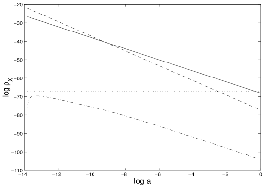
Figure 1.2: Evolution of $\log\rho_{m}$ (solid lines) , $\log\rho_{\psi}$ (dash-dotted line), $\log\rho_{\lambda}$ (dotted line) and $\log\rho_{r}$ (dashed line) as a function of $\log(a)$.

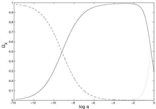
Figure 1.3: Evolution of $\log\rho_{m}$ (solid lines) , $\log\rho_{\psi}$ (dash-dotted line), $\log\rho_{\lambda}$ (dotted line) and $\log\rho_{r}$ (dashed line) as a function of $\log(a)$.

The inclusion of a varying-$\alpha$ will then affect very little the cosmological expansion of the universe. Hence, the Hubble diagram will be precisely the same as that of a universe, with a constant $\alpha$, with $\Omega_{m}\approx 0.3$, $\Omega_{\Lambda}\approx 0.7$ and $h=0.65$ [107]. This is the effect that we desired in a varying-$\alpha$ model: the less possible deviations from the standard FRW universe.

Chapter 2 Background Solutions for the Fine Structure Constant

Finjo viver num tempo sem fim
e de tanto fingir…
esqueci-me que só sei viver assim
– Ernesto Mota –

2.1 Introduction

In the last chapter we have described the BSBM varying-$\alpha$ cosmological model we will use to study the effect of the matter inhomogeneities in the cosmological evolution of the fine structure constant. Before starting to investigate those effects, we first need to study the evolution of $\alpha$ in the homogeneous and isotropic background universe and to calculate analytical solutions of the equation of motion (1.7.8) for $\psi$. These analytical solutions will be useful when we study the existence and behaviour of the inhomogeneities.

We will then provide a complete analysis of the behaviour of the solutions of the non-linear propagation equation (1.7.8) for appropriate behaviours of $a(t)$, for each epoch the universe went through: radiation dominated, dust dominated and dark energy dominated.

The aim of this chapter brings a question: How shall we solve the non-linear differential equation (1.7.8)? One cannot hope to obtain exact solutions to most non-linear differential equations. The reason is that there are only a limited number of systematic procedures for solving them, and these apply only to a very restricted class of equations. Moreover, even when a closed-form solution is known, it may be so complicated that its qualitative properties are obscure. Thus, for most non-linear equations it is necessary to have reliable techniques to determine the approximate behaviour of the solutions. In order to calculate and to understand the exact solutions of equation (1.7.8), we will use a phase-space analysis. From this analysis, we will be able to find stable asymptotic solution which can be considered to describe the behaviour of $\psi$ during the different eras the universe went through.

2.2 An Approximation Method

We have seen in the last chapter, that the energy density of the field associated to variations of $\alpha$ is always negligible with respect to all the other energy content of the universe ($\rho_{\psi}\ll\rho_{m},\rho_{r},\rho_{\Lambda}$). This means the Friedmann models with varying $\alpha$ have the property that the homogeneous motion of the $\psi$ does not create significant metric perturbations at late times [108]. So, far from the initial singularity, we can safely assume that the expansion scale factor follows the form for the Friedmann universe containing the same fluid when $\alpha$ does not vary $(\zeta=0=\psi)$. The behaviour of $\psi$ then follows from a solution of equation (1.7.8) in which $a(t)$ has the form for a Friedmann universe for matter with the same equation of state in general relativity when $\zeta=0=\psi.$ This behaviour is natural. We would not expect that very small variations of the coupling to electromagnetically interacting matter would have large gravitational effects upon the expansion of the universe. Thus, in this chapter we will provide a complete analysis of the behaviour of the solutions of equation (1.7.8) for appropriate behaviours of $a(t).$

Before starting the analysis and to calculate the asymptotic exact solutions let us show that the assumptions we claim are indeed right. Hence, we will show how good is the approximation of assuming that the scale factor, $a(t)$, will not deviate from the the usual FRW universe that we have calculated in the previous chapter, see table 1.1.

We consider spatially flat universes ($k=0$) and assume that the expansion scale factor is that of the Friedmann model containing a perfect fluid:

$$a=t^{n}$$ (2.2.1)

where $n$ is a constant. The late stages of an open universe containing fluid with density $\rho$ and pressure $p$ obeying $\rho+3p>0$ can be studied by considering the case $n=1.$ We rewrite the wave equation (1.7.8) as

$$\ (\dot{\psi}a^{3}\dot{)}=-\frac{2\zeta}{\omega}\rho_{m}a^{3}\exp[-2\psi]$$

Therefore, since $\rho_{m}a^{3}$ is constant this reduces to a Liouville equation of the form

$$(\dot{\psi}a^{3})^{.}=\ N\exp[-2\psi]$$ (2.2.2)

where $N$ is a constant, defined by

$$N\equiv-\frac{2\zeta}{\omega}\rho_{m}a^{3}\ .$$ (2.2.3)

We shall consider first the cosmological models that arise when the defining constant $N$ is negative. This arises when the constant $\zeta<0,$ indicating that the matter content of the universe is dominated by magnetic rather than electrostatic energy. The value of $\zeta$ for baryonic and dark matter has been disputed [56, 57, 107]. It is the difference between the percentage of mass in electrostatic and magnetostatic forms. As explained in the previous chapter and [107], we can at most estimate this quantity for neutrons and protons, with $\zeta_{n}\approx\zeta_{p}\sim 10^{-4}$. We may expect that for baryonic matter $\zeta\sim 10^{-4}$, with composition-dependent variations of the same order. The value of $\zeta$ for the dark matter, for all we know, could be anything between -1 and 1. Superconducting cosmic strings, or magnetic monopoles, display a negative $\zeta$, unlike more conventional dark matter. It is clear that the only way to obtain a cosmologically increasing $\alpha$ in BSBM is with $\zeta<0$, i.e with unusual dark matter, in which magnetic energy dominates over electrostatic energy. In [107] it was showed that fitting the Webb et al results requires $\zeta/\omega=-2\pm 1\times 10^{-4}$, where $\zeta$ is weighted by the necessary fractions of dark and baryonic matter required by observations of the gravitational effects of dark matter and the calculations of Big Bang nucleosynthesis. We note also that in practise $\zeta$ might display a significant spatial variation because of the change in the nature of the dominant form of matter over different length scales. For example, a magnetically dominated form of dark matter might contribute a negative value of $\zeta$ on large scales while domination of the matter content by baryons on small scales would lead to $\zeta>0$ locally. We will not investigate the effects of such variations in this thesis.

2.2.1 The validity of the approximation

We have assumed that the scale factor is given by the FRW model and then solved the $\psi$ evolution equation. This is a good approximation up to logarithmic corrections. Here is what happens to higher order.

We take the leading order behaviour in (1.7.7)

$$\left(\frac{\dot{a}}{a}\right)^{2}\approx\frac{8\pi}{3}\rho_{m}\left(1+\left|\zeta\right|e^{-2\psi}\right)$$ (2.2.4)

Now if we take $a=t^{2/3}$ so

$$\frac{8\pi}{3}\rho_{m}=\frac{4}{9t^{2}}$$

and solve equation (2.2.2) we get asymptotically,

$$\psi=\frac{1}{2}\ln[2N\ln t]\rightarrow\ln[\ln t]$$ (2.2.5)

to leading order at late times. Suppose we now re-solve (2.2.4) with the $\left|\zeta\right|e^{-2\psi}$ correction included

$$\left(\frac{\dot{a}}{a}\right)^{2}\approx\frac{4}{9t^{2}}\ \left(1+\left|\zeta\right|e^{-2\psi}\right)\approx\frac{4}{9t^{2}}\left(1+\frac{\left|\zeta\right|}{\ \ln t}\right)$$ (2.2.6)

Note that the kinetic term which we neglected is of order

$$\omega\dot{\psi}^{2}\sim\frac{1}{4t^{2}\ln^{2}t}$$ (2.2.7)

and so is smaller than the term we have retained. Solving equation (2.2.4) we have

$$\ln a=\frac{2\left|\zeta\right|}{3}\left[sh^{-1}\left\{\sqrt{\frac{\ln t}{\left|\zeta\right|}}\right\}+\sqrt{\frac{\ln t}{\left|\zeta\right|}}\sqrt{1+\frac{\ln t}{\left|\zeta\right|}}\right]$$ (2.2.8)

Note that when $\left|\zeta\right|\rightarrow 0$ this gives the usual $\ln a=\frac{2}{3}\ln t$. When $\left|\zeta\right|\neq 0$ we have

$$\ln a\rightarrow\frac{2\left|\zeta\right|}{3}\left\{\ln[2\sqrt{\frac{\ln t}{\left|\zeta\right|}}]+\frac{\ln t}{\left|\zeta\right|}\right\}$$

and

$$a=t^{2/3}(\ln t)^{\left|\zeta\right|/3}$$ (2.2.9)

where $\left|\zeta\right|$ is small and so the corrections to the $a=t^{2/3}$ ansatz are small. In terms of the Hubble rate:

$$H=\frac{2}{3t}+\frac{\left|\zeta\right|}{3t\ln t}$$

If we include the kinetic corrections to equation (2.2.4) then as $\dot{\psi}=\frac{1}{2t\ln t}$

$$\left(\frac{\dot{a}}{a}\right)^{2}\approx\frac{4}{9t^{2}}\ \left(1+\left|\zeta\right|e^{-2\psi}\ \right)+\frac{4\pi\omega}{3}\dot{\psi}^{2}\approx\frac{4}{9t^{2}}\left(1+\frac{\left|\zeta\right|}{\ \ln t}+\frac{S}{\ \ln^{2}t}\right)$$ (2.2.10)

where

$$S\equiv\frac{3\pi\omega}{4}$$

So, if $x=\ln t,$ we have

$$\frac{3}{2}\ln a = \sqrt{x^{2}+\left|\zeta\right|x+S}+S\int\frac{dx}{x\sqrt{x^{2}+\left|\zeta\right|x+S}}$$ (2.2.11)

$$+\frac{\left|\zeta\right|}{2}\int\frac{dx}{\sqrt{x^{2}+\left|\zeta\right|x+S}}$$

$$\frac{3}{2}\ln a = \sqrt{x^{2}+\left|\zeta\right|x+S}-\ln\left[\frac{2S+\left|\zeta\right|x+2\sqrt{S}\sqrt{x^{2}+\left|\zeta\right|x+S}}{x}\right]$$ (2.2.12)

$$+\frac{\left|\zeta\right|}{2}\ln\left[2\sqrt{x^{2}+\left|\zeta\right|x+S}+2x+\left|\zeta\right|\right]$$

Again, as $t\rightarrow\infty$ the leading order behaviour is that found in equation (2.2.9).

In the radiation era, where $a(t)\propto t^{1/2}$, we have an exact solution of equation (2.2.2) with

$$2\psi=\ln(8N)+\frac{1}{2}\ln t$$ (2.2.13)

so the corrections to the Friedmann equation look like

$$\left(\frac{\dot{a}}{a}\right)^{2}\approx\frac{1}{4t^{2}}\ \left(1+\left|\zeta\right|e^{-2\psi}\right)\approx\frac{1}{4t^{2}}\left(1+\frac{\left|\zeta\right|}{8N\ t^{1/2}}\right)$$ (2.2.14)

and these corrections fall off much faster than in the dust case. Again, our basic approximation method holds good to high accuracy.

2.2.2 A linearisation instability

Despite the robustness of the basic test-motion approximation that we are employing to analyse the evolution of $\psi(t)$ as the universe expands, there is a subtle feature the non-linear evolution equation (2.2.2) which must be noted in order that spurious conclusions are not drawn from an approximate analysis. We see that the right-hand side of equation (2.2.2 ) is always positive. Therefore $\psi$ can never experience an expansion maximum (where $\dot{\psi}=0$ and $\ddot{\psi}<0$) and therefore $\psi(t)$ can never oscillate. However, if we were to linearise equation (2.2.2), obtaining

$$(\dot{\psi}a^{3})^{.}=\ N\exp[-2\psi]\approx N(1-2\psi+O(\psi^{2}))$$

then for $\psi>1/2$ the right-hand side takes negative values and pseudo-oscillatory solutions for $\psi$ would appear that are not the linearised approximation to any true solution of the non-linear equation ( 2.2.2). Care must therefore be taken to ensure that analytic approximations are not extended to large $\psi$ and that numerical analyses are not creating spurious spirals in the phase plane by virtue of a linearisation procedure; for a fuller discussion see ref. [110].

These considerations can be taken further. It is possible for $\psi(t)$ to decrease, reach a minimum and then increase. But it is not possible for $\psi(t)$ to decrease if it has ever increased. A second interesting consequence of this feature of equation (2.2.2) is that it holds true even if $a(t)$ reaches an expansion maximum and begins to contract. Thus in a closed universe we expect $\psi$ and $\alpha$ to continue to increase slowly even after the universe begins to contract. This will have important consequences for the expected variation of $\psi$ and $\alpha$ in realistically inhomogeneous universes.

2.3 Two-Dimensional Non-Linear Autonomous Systems

Autonomous systems of equations, when they are interpreted as describing the motion of a point in the phase space, are particularly susceptible to some very beautiful techniques of local analysis. By performing a local analysis of the system near what are know as critical points, one can make remarkably accurate predictions about the global behaviour of the solution.

In this section, we shall not attempted to give a proper description of the the dynamical systems field, but we will only state the basic results needed to understand this chapter. For a better and proper study of the topic see for instance [130, 131, 132].

Differential equations which do not contain the independent variable explicitly are said to be autonomous. Any differential equation is equivalent to an autonomous equation of one higher order.

It is convenient to study the approximate behaviour of an autonomous equation of order $2$ when it is in the form of a system of $2$ coupled first-order differential equations. The general form of such a system is

$$\dot{y}_{1} = f_{1}(y_{1},y_{2})$$

$$\dot{y}_{2} = f_{2}(y_{1},y_{2})$$ (2.3.1)

where the dots indicate a differentiation with respect to the independent variable, for instance $t$.

The solution of the system (2.3.1) is a curved or trajectory in a two-dimensional space called phase space. The trajectory is parametrised in terms of $t:y_{1}=y_{1}(t)$, $y_{2}=y_{2}(t)$.

We assume that $f_{1}$, $f_{2}$ are continuous differentiable with respect to each of their arguments. Thus, by the existence and uniqueness theorem of differential equations [130] any initial condition $y_{1}(0)=a_{1}$, $y_{2}(0)=a_{2}$, gives rise to a unique trajectory through the point $(a_{1},a_{2})$. To understand this uniqueness property geometrically, note that every point on the trajectory $[y_{1}(t),y_{2}(t)]$, the system (2.3.1) assigns a unique velocity vector $[\dot{y}_{1}(t),\dot{y}_{2}(t)]$ which is tangent to the trajectory at that point. It immediately follows that two trajectories cannot cross; otherwise, the tangent vector at the crossing point would not be unique.

2.3.1 Critical points in phase space

If there are any solutions to the set of simultaneous algebraic equations

$$f_{1}(y_{1},y_{2}) = 0\qquad(\Leftrightarrow\dot{y}_{1}=0)$$

$$f_{2}(y_{1},y_{2}) = 0\qquad(\Leftrightarrow\dot{y}_{2}=0)\$$ (2.3.2)

then there are special degenerate trajectories in phase space which are just points. The velocity at these points is zero so the position vector does not move. These points are called critical points.

Studying the phase space it is possible to make elegant global analyses of the system. The possible behaviours of a trajectory in a two dimensional system [130] are:

• The trajectory may approach a critical point as $t\rightarrow+\infty$.

• The trajectory may approach $\infty$ as $t\rightarrow+\infty$.

• The trajectory may remain motionless at a critical point for all $t$.

• The trajectory may describe a closed orbit or a cycle.

• The trajectory may approach a closed orbit (by spiralling inward or outward toward the orbit) as $t\rightarrow+\infty$.

The possible local behaviours for trajectories near a critical point are:

• 1. All trajectories may approach the critical point along curves which are asymptotically straight lines as $t\rightarrow+\infty$. We call such a critical point a stable node.

• 2. All trajectories may approach the critical point along spiral curves as $t\rightarrow+\infty$. Such a critical point is called a stable spiral point.

• 3. All time reversed trajectories, that is, $y(t)$ with $t$ decreasing, may move toward the critical point along paths which are asymptotically straight lines as $t\rightarrow-\infty$. Such a critical point is an unstable node. As $t$ increases, all trajectories that start near an unstable node move away from the node along paths that are approximate straight lines, at least until the trajectory gets far from the node.

• 4. All time-reversed trajectories may move forward the critical point along spiral curves as $t\rightarrow-\infty$. Such a critical point is called an unstable spiral point. As $t$ increases, all trajectories move away from an unstable spiral point along trajectories that are, at least initially, spiral shaped.

• 5. Some trajectories may approach the critical point while others move away from it as $t\rightarrow+\infty$. Such a critical point is called a saddle point.

• 6. All trajectories may form a closed orbit about the critical point. Such a critical point is called a centre.

2.3.2 Matrix methods

Linear autonomous systems

Since two-dimensional linear autonomous systems can exhibit any of the critical point behaviours that we have described above, it is appropriate to study linear systems before going to non-linear ones. With this in mind we introduce an easy method for solving linear autonomous systems.

A two dimensional linear autonomous system $\dot{y}_{1}=ay_{1}+by_{2}$, $\dot{y}_{2}=cy_{1}+dy_{2}$ may be re-written in matrix form as

$${\bf{\dot{Y}}}=M{\bf{Y}}$$ (2.3.3)

where $M=\bordermatrix{&&\cr&a&b\cr&c&d\cr}$   and   ${\bf{Y}}=\bordermatrix{&\cr&y_{1}\cr&y_{2}\cr}$

It is easy to verify that if the eigenvalues $\lambda_{1}$ and $\lambda_{2}$ of the matrix $M$ are distinct and ${\bf{V_{1}}}$ and ${\bf{V_{2}}}$ are eigenvectors of $M$ associated to the eigenvalues $\lambda_{1}$ and $\lambda_{2}$, then the general solution to equation (2.3.3) has the form

$${\bf{Y}}(t)=c_{1}{\bf{V_{1}}}e^{\lambda_{1}t}+c_{2}{\bf{V_{2}}}e^{\lambda_{2}t}$$ (2.3.4)

where $c_{1}$ and $c_{2}$ are constants of integration which are determined by the initial position ${\bf{Y}}(0)$.

The linear system (2.3.3) has a critical point at the origin $(0,0)$. It is easy to classify this critical point once $\lambda_{1}$ and $\lambda_{2}$ are known. Note that, $\lambda_{1}$ and $\lambda_{2}$ satisfy the eigenvalue condition

$det[M-I\lambda]=det\bordermatrix{&&\cr&a-\lambda&b\cr&c&d-\lambda\cr}$ = $\lambda^{2}-\lambda(a+d)+ad-bc=0$

If $\lambda_{1}$ and $\lambda_{2}$ are real and negative, then all trajectories approach the origin as $t\rightarrow\infty$ and $(0,0)$ is a stable node. Conversely, if $\lambda_{1}$ and $\lambda_{2}$ are real and positive, then all trajectories move away from $(0,0)$ as $t\rightarrow\infty$ and $(0,0)$ is an unstable node. Also, if $\lambda_{1}$ and $\lambda_{2}$ are real but $\lambda_{1}$ is positive and $\lambda_{2}$ is negative, then $(0,0)$ is a saddle point; trajectories approach the origin in the ${\bf{V_{2}}}$ direction and move away from the origin in the direction ${\bf{V_{1}}}$.

Solutions $\lambda_{1}$ and $\lambda_{2}$ of (2.3.2) may be complex. However, when the matrix $M$ is real, then $\lambda_{1}$ and $\lambda_{2}$ must be a complex conjugate pair. If $\lambda_{1}$ and $\lambda_{2}$ are pure imaginary, then the vector ${\bf{Y}}(t)$ represents a closed orbit for any $c_{1}$ and $c_{2}$ and the critical point at $(0,0)$ is a centre. If $\lambda_{1}$ and $\lambda_{2}$ are complex with non-zero real part, then the critical point at $(0,0)$ is a spiral. When $Re$ $\lambda_{1,2}<0$, then ${\bf{Y}}(t)\rightarrow 0$, $(0,0)$ is a stable spiral point; conversely, when $Re$ $\lambda_{1,2}>0$, $(0,0)$ is an unstable spiral point.

Two-dimensional non-linear systems

The analysis of a non-linear system is a much more complicate case. Nevertheless non-linear system can be analysed near its critical points, and the result of that study can be indeed very accurate if the system is almost linear. In our particular case, the condition for almost-linearity can be checked comparing our results with the numerical integrations performed in [108]. We will see that our results are indeed very good approximation to the solutions found numerically, with exception to one case where one of the eigenvalue solution of equation (2.3.2) is zero. The stability analysis of this case will be described bellow in 2.3.2.

The local analysis of a non-linear system, to which the linear approximation works well, consist into linearise the equations and then procedure as usually done for a linear system. We first identify the critical points. Then we perform, a local analysis of the system very near them. Using matrix methods, we identify the nature of the critical points of the linear system. Finally, we assemble the results of our local analysis and synthesise a qualitative global picture of the solution to the non-linear system.

Critical point with one zero eigenvalue

In this section we will only present the results obtained in [133] and we refer the reader to that reference for a detailed explanation.

If one of the eigenvalue solutions, $\lambda_{1,2}$, of equation (2.3.2) has, for instance, $Re(\lambda_{1})=0$ and $Re(\lambda_{2})<0$ then the stability cannot be decided by the linear approximation.

In general, a non-linear autonomous system can be written in the form

$${\bf\dot{Y}}=M{\bf Y}+N({\bf Y})$$ (2.3.5)

where $M$ is a constant matrix $2\times 2$ and $N({\bf Y})$ is non-linear in ${\bf Y}$. The linearisation of this system gives (2.3.3). Consider now that, the two eigenvalues of $M$, have $Re(\lambda_{1})=0$ and $Re(\lambda_{2})<0$, corresponding to the eigenvectors ${\bf{V_{1}}}$ and ${\bf{V_{2}}}$. In order to perform the stability analysis of the critical point $(0,0)$, we should procedure as follows (For other alternatives to this method see [131]).

• First, we apply a linear transformation to ${\bf Y}$ using the matrix formed by the eigenvectors ${\bf{V_{1}}}$ and ${\bf{V_{2}}}$. This will split the system into critical and non-critical variables; the critical variable is the eigenvector corresponding to $Re(\lambda_{1})=0$, in our case ${\bf{V_{1}}}$. Hence, ${\bf{Y}}\rightarrow{\bf{X}}=(x_{1},x_{2})$. In the new coordinates, we now have that the following system

  $$\dot{x}_{1} = n_{1}(x_{1},x_{2})$$

  $$\dot{x}_{2} = p_{21}x_{1}+\bar{p}_{2}x_{1}+n_{2}(x_{1},x_{2})$$ (2.3.6)

  where $n_{1}$ and $n_{2}$ are at least quadratic in both $x_{1}$ and $x_{2}$.

• Secondly, if there are linear terms in $x_{1}$, in the above system, then they must be eliminated. That can be achieved solving the equation $\dot{x}_{2}=0$, which will give us $x_{2}$ has a function of $x_{1}$ (the critical variable). Say, for instance, that solution give $x^{*}_{2}(x_{1})$.

• At last, we perform the following transformation $(x_{1},x_{2})\rightarrow(z_{1},z_{2})$ defined as

  $$(z_{1},z_{2})=\left(x_{1},x_{2}-x_{2}^{*}\left(x_{1}\right)\right)$$ (2.3.7)

Having performed this steps we end up with an autonomous system for the coordinates $(z_{1},z_{2})$

$$\dot{z}_{1} = h_{1}(z_{1},z_{2})$$

$$\dot{z}_{2} = p_{21}x_{1}+h_{2}(z_{1},z_{2})$$ (2.3.8)

where the functions $h_{1}$ and $h_{2}$ are at least quadratic in their arguments. the stability of the critical point ${\bf{Y}}=(0,0)$ is determined by the stability of ${\bf{Z}}\equiv(z_{1},z_{2})=(0,0)$.

Since the non-null eigenvalue of $M$ has a negative real part ($Re(\lambda_{2})<0$, by assumption), the coordinate $z_{2}$ is asymptotically stable about the origin $(0,0)$ as $t\rightarrow\infty$. The asymptotic stability of the critical variable is therefore determined as $t\rightarrow\infty$ and $z_{2}\rightarrow 0$ by the leading term of $h_{1}(z_{1},0)$. It can be shown [133] that when the first power of $h_{1}(z_{1},0)$ is even (recall that $h_{1}$ is at least a quadratic function), then $(z_{1},z_{2})=(0,0)$ is unstable.

2.4 Phase-Plane Analysis

We are ready now to analyse the phase space of equation (2.2.2). We first transform it into an autonomous system of two first order differential equations. Then we identify the critical points and we perform, a local analysis of the system very near them. The exact system will be well approximated by a linear autonomous system near the critical points. This will be seen when we compare our results with the numerical results performed in [108]. Using matrix methods we identify the nature of the critical points of the linear system. Finally, we assemble the results of our local analysis and synthesise a qualitative global picture of the solution to the non-linear system.

2.4.1 A transformation of variables

In this section we will look at the $\psi$ equation of motion (2.2.2 ) when the expansion scale factor takes the power-law form (2.2.1). The evolution equation for the field then becomes:

$$\frac{d}{dt}\left(\dot{\psi}t^{3n}\right)=N\exp[-2\psi]$$ (2.4.1)

with $N>0.$ We introduce the following variables :

$$x=ln(t)\qquad y=\psi-Ax-B\qquad A=1-\frac{3n}{2}\qquad B=\frac{1}{2}\ln(N)$$ (2.4.2)

and rewrite (2.2.2) as:

$$y^{\prime\prime}+(3n-1)(y^{\prime}+1-\frac{3n}{2})=e^{-2y},$$ (2.4.3)

where ^′ $\equiv d/dx$. This second-order differential equation can be transformed into an autonomous system by defining $v=\frac{dy}{dx}$ and $u=y$:

$$\frac{dv}{dx} = e^{-2u}+(1-3n)(v+1-\frac{3n}{2})$$ (2.4.4)

$$\frac{du}{dx} = v$$

With the aim to obtain asymptotic exact solution, we have to search for the critical points of equation (2.4.4). The critical points of a system are defined as the values of $u$ and $v$ that give $v^{\prime}=0$ and $u^{\prime}=0$, where the prime represents a derivative with respect to $x$. The importance of the critical points is the fact that we can linearise the system around then, and if they are stable, the solution of the system near them, can be used as an asymptotically stable solution.

Looking at equation (2.4.4), it is straight forward to see that the system has a finite critical point at

$$(u_{c},v_{c})=(-\frac{1}{2}\ln{[(1-3n)(\frac{3n}{2}-1)]},0)$$ (2.4.5)

when $n\in(\frac{1}{3},\frac{2}{3})$ and it has a infinite critical point at $(u_{c},v_{c})=(+\infty,0)$ when $n=\frac{1}{3}$ or $n=\frac{2}{3}$. The finite critical points correspond to the family of exact solutions of the form $\psi=B+A\ln(t)$ found in [108]. In the original variables these solutions are

$$\psi=\frac{1}{2}\ln[\frac{2N}{(2-3n)(3n-1)}]+\left(\frac{2-3n}{2}\right)\ln(t).$$

In order to analyse the system fully, we will study finite critical points and the critical points at infinity separately. We will also distinguish several domains of behaviour for $n$: $n=\frac{1}{3}$, $n=\frac{2}{3}$, $n\in(\frac{1}{3},\frac{2}{3})$, $n<\frac{1}{3}$ and $n>\frac{2}{3}$. In some cases we will supplement our investigations by numerical study of the system (2.4.4).

2.4.2 The finite critical points

The cases $n\in(\frac{1}{3},\frac{2}{3})$

In the domain where $n\in(\frac{1}{3},\frac{2}{3})$ the system (2.4.4) does not appear to be exactly integrable. So in this section we will study the behaviour of the system near the critical points and at late times.

There is a finite critical point $(u_{c},v_{c})=(-\frac{1}{2}\ln{[(1-3n)(\frac{3n}{2}-1)]},0)$ for $n\in(\frac{1}{3},\frac{2}{3})$. Linearising the system 2.4.4 about it we obtain:

$$\frac{dV}{dx} = (3n-1)(3n-2)U+(1-3n)V$$ (2.4.6)

$$\frac{dU}{dx} = V$$

where $V=v-v_{c}$ and $U=u-u_{c}$. Since the characteristic matrix is non singular the critical point is simple. Hence the non-linearised version of this system has the same phase portrait at the neighbourhood of the critical point.

The eigenvalues $\xi_{1,2}$ and corresponding eigenvectors $\chi^{\xi_{1,2}}$ of the system (2.4.6) are:

$$\xi_{1,2} = {\frac{1-3n\pm\sqrt{9-42n+45{n^{2}}}}{2}}$$ (2.4.7)

$$\chi^{\xi_{1,2}} = ({\frac{1-3n\pm\sqrt{9-42n+45{n^{2}}}}{2}},1)$$

These eigenvalues will be complex numbers for $n\in(\frac{1}{3},\frac{3}{5})$ and they will be pure real numbers when $n\in(\frac{3}{5},\frac{2}{3})$. Notice that for both cases the real part of the eigenvalues is always negative, so the critical point is a stable attractor. The general solution of the linearised system (2.4.6) can be expressed as:

$$(U(x),V(x))=A{e^{\xi_{1}x}}\chi_{1}+B{e^{\xi_{2}x}}\chi_{2}$$

where $A$, $B$ are arbitrary constants and $x=\ln(t)$. From the transformations (2.2.2) we can obtain explicitly the expression for $\psi(t)$ near the critical point. There are three possible behaviours of the solutions near the critical point:

Pseudo-oscillatory $\psi$ behaviour

When $n\in(\frac{1}{3},\frac{3}{5})$ the linearised evolution for the $\psi$ field exhibits damped oscillations about its asymptotic solution as $t\rightarrow\infty$:

$$\psi(t) = \frac{1}{2}\ln[\frac{2N}{\left(1-3n\right)\left(3n-2\right)}]+\frac{1}{2}\left(2-3n\right)\ln(t)$$

$$+{t^{\alpha}}\left(B\cos[\beta\ln(t)]+A\sin[\beta\ln(t)]\right)$$

where

$$\alpha = {\frac{1-3n}{2}}$$ (2.4.9)

$$\beta = {\frac{\sqrt{9+42n-45{n^{2}}}}{2}}$$ (2.4.10)

We note that this family of solutions and asymptotes includes the case of the radiation-dominated universe ($n=1/2$). The phase portrait and the $\psi$ vs. $\ln t$ for this case are shown in figure 2.1. But in the case of a universe containing the balance of matter and radiation, displayed by our own, it need not be the case that the asymptotic behaviour, displayed by the exact solution for the critical point, is reached before the radiation-dominated expansion is replaced by matter-domination, see references [107] and [108] for further discussion of this point. However as we discussed above these oscillations are an artifact of the linearisation process and the part of the solution ( 2.4.2) controlled by the constants $A$ and $B$ is only valid for small times, hence we called this behaviour pseudo-oscillatory.

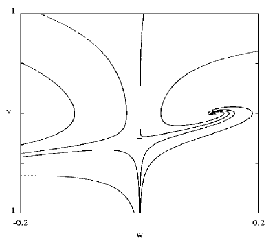
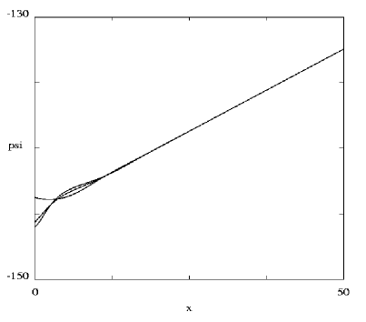
Figure 2.1: Numerical plots of the phase space in the $(w,v)$ coordinates, and the $\psi$ evolution with $x=log(t)$ for $n=\frac{1}{2}$ .The ’$+$’ sign is a saddle point and the triangle is a stable node.

Non-oscillatory behaviour

When $n\in(\frac{3}{5},\frac{2}{3})$, the $\psi$ field will approach its asymptotic behaviour in a non-oscillatory fashion as $t\rightarrow\infty$:

$$\psi(t) = \frac{1}{2}\ln[\frac{2N}{\left(1-3n\right)\left(3n-2\right)}]$$

$$+\frac{1}{2}\left(2-3n\right)\ln(t)+t^{\delta-\gamma}\left(A+B{t^{2\gamma}}\right)$$

where

$$\delta = {\frac{1-3n}{2}}$$ (2.4.12)

$$\gamma = \frac{1}{2}\sqrt{9-42n+45{n^{2}}}$$ (2.4.13)

Note that $\delta+\gamma<0$ in the domain $n\in(\frac{1}{3},\frac{2}{3})$ , so at late times ($t\rightarrow\infty$), both the pseudo-oscillatory and non-oscillatory solutions case will approach the asymptotic solution defined by the appropriate value of $n$.

Intermediate behaviour

A transition between the pseudo-oscillatory and non-oscillatory regimes happens when $\beta=0$ and $n=\frac{3}{5}$; the $\psi$ field then has the following solution in the vicinity of the critical point:

$$\psi(t)=\frac{1}{5}\ln(N)+\frac{1}{10}\ln(t)+At^{-{\frac{2}{5}}}.$$ (2.4.14)

The phase plane structure and evolution of $\psi$ vs. $\ln t$ for this case are shown in figure 2.2.

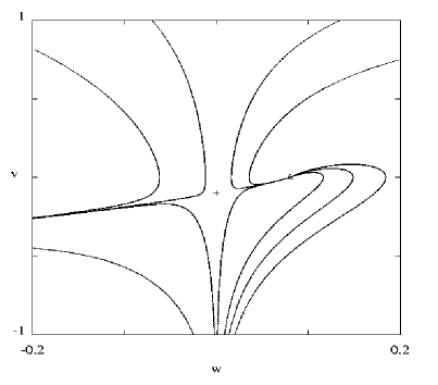
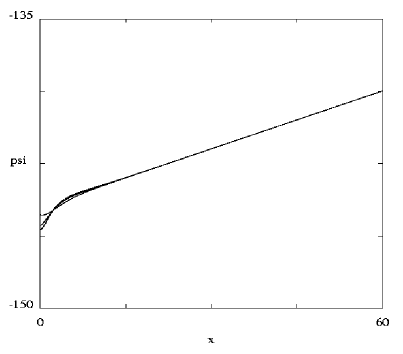
Figure 2.2: Numerical plots of the phase space in the $(w,v)$ coordinates, and the $\psi$ evolution with $x=log(t)$ for $n=\frac{3}{5}$. The ’$+$’ sign is a saddle point and the triangle is a stable node.

Overview

The late-time solution of the $\psi$ field solution is given by asymptotic behaviour of equations (2.4.2) or (2.4.2), which is:

$$\psi\rightarrow\frac{1}{2}\ln[\frac{2N}{\left(1-3n\right)\left(3n-2\right)}]+\frac{1}{2}\left(2-3n\right)\ln(t)$$

This shows that the solutions (2.4.2) and (2.4.2) generalise the ones found in [108], since they can be obtained setting $A=B=0$ in ( 2.4.2). In particular, the case of a radiation-dominated Universe ($n=\frac{1}{2}$), we have from (2.4.2):

$$\psi(t) = \frac{1}{2}\left(\log(8)+\log(N)+\log(t)\right)$$

$$+{t^{{-\frac{1}{4}}}}\left(B\cos[{\frac{5\sqrt{3}\log(t)}{4}}]+A\sin[{\frac{5\sqrt{3}\log(t)}{4}}]\right)$$

A full mathematical summary of the change in structure of the phase space with changing $n$ for the system (2.2.2) is given in section 2.6. There we include cosmologically unphysical values of $n$ and show how the critical point structure bifurcates with the change in value of $n$.

2.4.3 The critical points at infinity

In order to describe the qualitative evolution of the system, we must determine the behaviour of the system (2.4.4) near the critical point $(u_{c},v_{c})=(+\infty,0)$. In order to bring the critical point to a finite value, we define:

$$u=-\frac{1}{2}\ln(w)$$

Using the new coordinate $w$ we can re-write the system (2.4.4) as:

$$\frac{dw}{dx} = -2wv$$ (2.4.16)

$$\frac{dv}{dx} = \left(1-3n\right)\left(1-{\frac{3n}{2}}+v\right)+w$$

This system has critical points on the $(w,v)$ plane when $(0,-1+{\frac{3n}{2}})$ and $(\left(1-3n\right)\left({\frac{3n}{2}}-1\right),0).$ Note that the second critical point is just the same as the one we have analysed in the previous section. In this subsection we will then only analyse the critical point $(w_{c},v_{c})=(0,-1+{\frac{3n}{2}})$ since it corresponds to the case where $u\rightarrow+\infty$.

Proceeding as before, and linearising (2.4.16) about $(w_{c},v_{c})=(0,-1+{\frac{3n}{2}})$ we obtain:

$$\frac{dW}{dx} = (2-3n)W$$ (2.4.17)

$$\frac{dV}{dx} = W+(1-3n)V$$

where $V=v-v_{c}$ and $W=w-w_{c}$. Again, the characteristic matrix of the system is non singular, and the critical point is simple. Hence, system (2.4.17) will have the same phase portrait as (2.4.16) in the neighbourhood of the critical point.

The eigenvalues $\xi_{1,2}$ and corresponding eigenvectors $\chi^{\xi_{1,2}}$ of the system (2.4.17) are:

$$\xi_{1} = 1-3n,\hskip 72.26999pt\chi^{\xi_{1}}=(0,1)$$ (2.4.18)

$$\qquad\xi_{2} = 2-3n,\hskip 72.26999pt\chi^{\xi_{2}}=(1,1)$$ (2.4.19)

These eigenvalues are always real. The critical point is an attractive node for $n>\frac{2}{3}$, a saddle point when $n\in(\frac{1}{3},\frac{2}{3})$, and it will be an unstable point when $n<\frac{1}{3}$. The general solution of the system (2.4.16) in the neighbourhood of the critical point $(w_{c},v_{c})=(0,-1+{\frac{3n}{2}})$, can be expressed as:

$$(w(x)-w_{c},v(x)-v_{c})=A{e^{\xi_{1}x}}\chi_{1}+B{e^{\xi_{2}x}}\chi_{2}$$

where $A$, $B$ are arbitrary constants and $x=\ln(t)$. Therefore, near the critical point $(u_{c},v_{c})=(+\infty,0)$:

$$\psi(t)=\frac{1}{2}\ln(\frac{N}{B})$$ (2.4.20)

so the scalar field is constant.

Note that in the domain $n\in(\frac{1}{3},\frac{2}{3})$ this is just a transitory solution since the critical point is a saddle point. In the domain $n<\frac{1}{3}$ it is an unstable critical point, possibly relevant as an early-time solution to braneworld cosmologies in the high-density regime where the Hubble expansion rate of the universe is linearly proportional to the density, so $n=1/4$ for a braneworld containing radiation, $n=1/12$ for a massless scalar field, and $n=1/6$ for dust. However, in the $t\rightarrow 0$ limit the assumption that the $\dot{\psi}^{2}$ and $\zeta\exp[-2\psi]$ terms can be neglected in the Friedmann equation (1.7.7) will break down.

The cases of $n>2/3$ and de Sitter expansion

An interesting case exists when $n>\frac{2}{3}$, since the critical point is a stable attractor and so this means that the constant-$\psi$ behaviour (2.4.20) is the late-time attractor, in agreement with the conclusions of references [107] and [108]. This is an important feature of a universe which exhibits accelerated expansion in its late stages ($n>1$). It means that the present value of $\alpha$ is the asymptotic one. It also means that variations of $\alpha$ are turned off by the domination of the expansion dynamics by negative curvature or by any quintessence field [107], [108]. This property may provide important clues to explaining why our universe possesses small but finite curvature or quintessence energy today: if it did not then the fine structure constant would continue to increase until it was impossible for atoms and molecules to exist [109]

In the $n>2/3$ case we can find a detailed asymptotic solution for equation ( 2.4.1) which has the form

$$\psi=C+B(t+t_{0})^{1-3n}+\frac{N\exp[-2C]}{2-3n}(t+t_{0})^{2-3n}$$

with $C,t_{0}$ constants. We see immediately that for this solution $\psi$ approaches a constant as $t\rightarrow\infty$. Of particular interest is the case of a curvature-dominated open universe, which has $n=1$. The phase plane structure and the evolution of $\psi$ vs. $\ln t$ for this case are shown in figure 2.3.

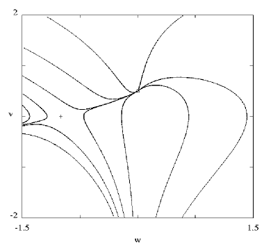
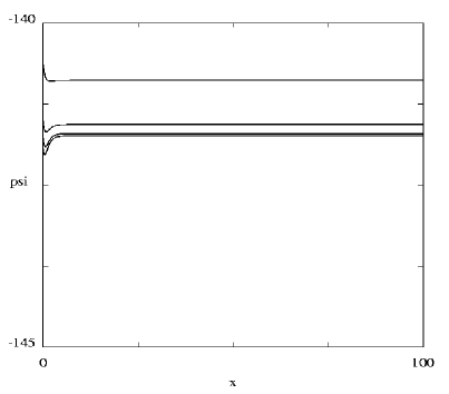
Figure 2.3: Numerical plots of the phase space in the $(w,v)$ coordinates, and the $\psi$ evolution with $x=log(t)$ for $n=1$. The ’$+$’ sign is a saddle point and the triangle is a stable node.

We see that this approach to constant behaviour occurs for all universes that accelerate ($n>1$) and so we would expect to find it also in the case of a de Sitter background universe with

$$a(t)=\exp[\lambda t]$$

where $\lambda>0$ is constant.

Substituting this in equation (2.2.2) we find a late-time asymptotic solution

$$\psi=C+B\exp[-3\lambda t]-\frac{N\left(3\lambda t+1\right)}{9\lambda^{2}}\exp[-2C-3\lambda t]\rightarrow C$$

as $t\rightarrow\infty.$

Notice that we were not able to fully describe the nature of this critical point in the cases where $n=\frac{1}{3}$ or $n=\frac{2}{3}$ since one of the eigenvalues of the systems is zero. In order to do so, we will study these two cases individually, in particular the case $n=\frac{2}{3}$ is important since it describes the scale factor evolution on a dust dominated universe.

The $n=\frac{1}{3}$, $a(t)=t^{\frac{1}{3}}$ case: an exact solution

The $n=\frac{1}{3}$ case can be exactly integrated. It is of interest as an exact solution in its own right but it corresponds to the case of a universe whose expansion dynamics are dominated by the effects of a fluid with a $p=\rho$ equation of state, or a massless scalar field. It also describes the behaviour of the $\psi$ field in an anisotropic universe of the simple Kasner type.

We see when $n=1/3$ the system (2.4.4) has the form:

$$\frac{dv}{dx} = e^{-2u}$$ (2.4.21)

$$\frac{du}{dx} = v$$

This integrates to give

$$v^{2}+e^{-2u}=E^{2}$$

where $E$ is a constant. Hence, we have two possible solution branches: $v(u)=\pm\sqrt{E-e^{-2u}}$. Both, positive ($+$) and negative ($-$) solutions for $v$ lead to the same result. Choosing the positive branch of the $v(u)$ solution and using equations (2.4.21) we obtain:

$$u(x)=-\ln(E)+\ln[\cosh\left(E\left(C_{1}-x\right)\right)]$$

where $C_{1}$ is an integration constant. From (2.4.2) we have a solution for $\psi(t)$:

$$\psi(t)={\frac{\ln(\frac{N}{4})\ }{2}}-\ln(E)+\frac{1}{2}\ln(t)+\ln[\exp[EC_{1}]t^{-E}+t^{E}\exp[-EC_{1}]]$$

and the asymptotic limit when $t\rightarrow\infty$ gives

$$\psi(t)\rightarrow(\frac{1}{2}+E)\ln(t+t_{0}).$$

with $t_{0}$ constant. The phase space and $\psi(t)$ vs. $\ln t$ evolution is shown in figure 2.4.

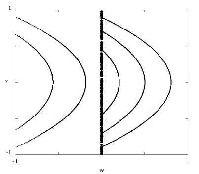
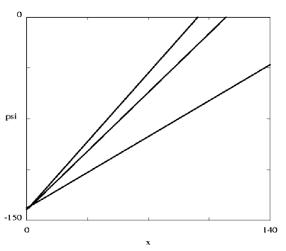
Figure 2.4: Numerical plots of the phase space in the $(w,v)$ coordinates and time evolution of $\psi(x)$ $n=\frac{1}{3}$. The central line which passes through the origin is an attractor for $w>0$, and an unstable line for $w<0$.

The $n=\frac{2}{3}$ , $a=t^{\frac{2}{3}}$ case

The case of a dust-dominated universe is mathematically special because of the presence of a zero eigenvalue in the stability analysis. It is illuminating to consider this case separately with an asymptotic analysis that extends the earlier study in [108].

Consider equation (2.4.1) with $n=2/3$. If we introduce the new variable $x=\ln(t),$ then

$$\psi^{\prime\prime}+\psi^{\prime}=N\exp[-2\psi]$$ (2.4.22)

At large $x$, the asymptotic form of this equation has the form:

$$\psi=\frac{1}{2}\ln[2N(x+x_{0})]-\frac{1}{2}\sum_{n=1}^{\infty}\frac{(n-1)!}{(x+x_{0})^{n}}+C\exp[-x]$$ (2.4.23)

where $C$ and $x_{0}>0$ are arbitrary constants. The leading order behaviour as $t\rightarrow\infty$ is therefore (cf.(2.2.5))

$$\psi\sim\frac{1}{2}\ln[2N\ln(t)]$$

Stability analysis of the $n=2/3$ asymptote

:

Performing the coordinate transformation $u=-\frac{1}{2}\ln(w)$ on the system (2.4.4) when $n=2/3$, we have:

$$\frac{dv}{dx} = w-v$$ (2.4.24)

$$\frac{dw}{dx} = -2vw$$

This system has a critical point at the origin of the $(w,v)$ plane. It corresponds to the case where $u\rightarrow\infty$. The linearisation about this critical point gives two eigenvalues: $\lambda_{1}=-1$ with the eigenvector $\chi_{1}=(0,1)$ and $\lambda_{2}=0$ with the eigenvector $\chi_{2}=(1,1)$. Since we have a zero eigenvalue, the stability is determined by the non-linear behaviour and is one of Lyapunov’s ’critical’ cases [133],[134] [132]. We apply a linear transformation to split the system into critical and non-critical variables; where the critical variables are those eigenvectors with zero eigenvalue and the non-critical variable are the others. Then we apply a non-linear transformation which will eliminate the influence of the critical variables upon the non-critical ones at the leading order. This gives $(w,v)\rightarrow(W,W+V)$, and the system (2.4.24) becomes:

$$W^{\prime} = -2W(W+V)$$ (2.4.25)

$$V^{\prime} = -V+2W(W+V)$$

with the critical point at $(W,V)=(0,0).$The Lyapunov procedure for the system (2.4.25) is to set the linearly stable variable, $V,$ equal to zero in the $W^{\prime}$ equation so,

$$W^{\prime}=-2W^{2}$$

and so the second-order analysis shows that critical point $(W,V)=(0,0)$ is unstable. In fact this critical point is a saddle point as can be seen from the numerical-phase-plane plot figure  2.5. The unstable part correspond to a non-physical range of the cosmological variables, since it gives $w<0$. The stable part corresponds to the range of values where $w\geq 0$. With respect to our (approximate) exact solution, the unphysical case will correspond to the range of $x_{0}<0$, since they lead to $\alpha<0$. Hence the asymptotic solution (2.4.23) is the stable late-time behaviour of the dust universes with small $\zeta.$ The phase plane structure and the evolution of $\psi$ vs. $\ln t$ is shown in figure 2.5.

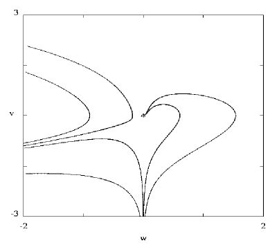
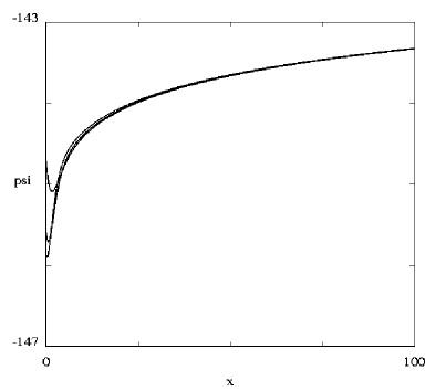
Figure 2.5: Numerical plots of the phase space in the $(w,v)$ coordinates, and the $\psi$ evolution with $x=log(t)$ for $n=\frac{2}{3}$. The triangle is a saddle point for $w<0$ and a stable node for $w>0$.

2.5 Some General Asymptotic Features

2.5.1 Models with asymptotically constant $\psi$ and $\alpha$

We have seen that $\psi$, and hence the fine structure constant, $\alpha$, tends to a constant at late times in accelerating universes with power-law and exponential increase of the scale factor. We can establish a useful general criterion for this asymptotic behaviour to occur for general $a(t)$. Suppose that as $t\rightarrow\infty$ both sides of equation (2.2.2) tend to a constant (which may be equal to zero). Thus

$$(\dot{\psi}a^{3})^{\cdot} = A$$

$$\psi = A\int\frac{tdt}{a^{3}}+B\int\frac{dt}{a^{3}}+C\rightarrow C$$

as $t\rightarrow\infty$ if

$$A\int\frac{tdt}{a^{3}} \rightarrow 0$$ (2.5.1)

$$B\int\frac{dt}{a^{3}} \rightarrow 0$$ (2.5.2)

Then for consistency we also require, as $t\rightarrow\infty$, that

$$N\exp[-2C]\rightarrow A$$

so $A$ cannot be chosen to be zero. Thus in all cosmological models for which (2.5.1) and (2.5.2) hold there will be a self-consistent asymptotic solution as $t\rightarrow\infty$ of the form

$$\psi=N\exp[-2C]\int\frac{tdt}{a^{3}}+B\int\frac{dt}{a^{3}}+C$$

where $B,C$ are positive constants. We see that the $n>2/3$ and de Sitter cases satisfy the conditions (2.5.1) and (2.5.2) hence $\psi$ is asymptotically constant. The dust ($n=2/3$) case, for which $\psi\rightarrow\infty$ as $t\rightarrow\infty$ satisfies (2.5.2) but violates (2.5.1).

2.6 General Analysis of the Phase Plane Bifurcations

In previous sections we have analysed the $\psi$ evolution equation (2.2.2) for a range of variables which are physically realistic and correspond to expanding universes. We will now analyse the whole range for variables of the system (2.4.17). As before we see there are two critical points in the $(w,v)$ plane, at $(0,-1+{\frac{3n}{2}})$ and $((1-3n)(\frac{3n}{2}-1),0)$. Linearising (2.4.17) about $(w_{c_{1}},v_{c_{1}})=(0,-1+\frac{3n}{2})$ and $(w_{c_{2}},v_{c_{2}})=((1-3n)(\frac{3n}{2}-1),0)$ we obtain the following characteristics matrices:

$M_{1}=\bordermatrix{&&\cr&2-3n&0\cr&1&1-3n\cr}$   $M_{2}=\bordermatrix{&&\cr&0&(3n-1)(2-3n)\cr&1&1-3n\cr}$

The characteristic matrices are non singular except when $n=\frac{1}{3}$ or $n=\frac{2}{3}$. In the non-singular cases the critical points will be simple and the system defined by these differential equations is structurally stable [130], and there will be no ’strange’ chaotic behaviour outside the neighbourhood of the critical points. Hence, the linearised system will have the same phase portrait as non-linearised one in the neighbourhood of the critical points.

The evolution, with respect to changing $n$, of the signs of the determinant and the trace of these two matrices is given in the table 2.1. This show us that there are always two critical points in our system, an unstable saddle and an attractor (which changes from a spiral to a node).

$n$	Critical Points $(w_{c},v_{c})$
	$\left(\left(3n-1\right)\left(1-\frac{3n}{2}\right),0\right)$	$\left(0,1-\frac{3n}{2}\right)$
$(-\infty;\frac{1}{3})$	Saddle Point (non-physical)	Unstable Node
	det $M_{1}<0$, Tr $M_{1}>0$	det $M_{2}>0$, Tr $M_{2}>0$
$\frac{1}{3}$	Origin	Axis
	det $M_{1}=0$, Tr $M_{1}=0$	det $M_{2}=0$, Tr $M_{2}>0$
$(\frac{1}{3};\frac{1}{2})$	Stable Spiral	Saddle Point
	det $M_{1}>0$, Tr $M_{1}<0$	det $M_{2}<0$, Tr $M_{2}>0$
$\frac{1}{2}$	Stable Spiral	Saddle Point
	det $M_{1}>0$, Tr $M_{1}<0$	det $M_{2}<0$, Tr $M_{2}=0$
$(\frac{1}{2};\frac{3}{5})$	Stable Spiral	Saddle Point
	det $M_{1}>0$, Tr $M_{1}<0$	det $M_{2}<0$, Tr $M_{2}<0$
$\frac{3}{5}$	Stable Spiral (node)	Saddle Point
	det $M_{1}>0$, Tr $M_{1}<0$	det $M_{2}<0$, Tr $M_{2}<0$
$(\frac{3}{5};\frac{2}{3})$	Stable Node	Saddle Point
	det $M_{1}>0$, Tr $M_{1}<0$	det $M_{2}<0$, Tr $M_{2}<0$
$\frac{2}{3}$	Stable Axis	Stable Axis
	det $M_{1}=0$, Tr $M_{1}<0$	det $M_{2}=0$, Tr $M_{2}<0$
$(\frac{2}{3};\infty)$	Saddle Point (non-physical)	Stable Node
	det $M_{1}<0$, Tr $M_{1}<0$	det $M_{2}>0$, Tr $M_{2}<0$

Table 2.1: Stability of all the critical points of the equation of motion for $\psi$.

The cases $n=\frac{1}{3}$ or $n=\frac{2}{3}$, where the determinant of the characteristic matrices vanishes, lead to a bifurcation of codimension $1$, in particular, of Saddle-Node type [131], since they correspond to points where the determinants of the characteristic matrices change sign, det $M_{1}$ $=$ det$M_{2}=0$. At these values of $n$ the nature of the system will change. Cosmologically, these points represent a change in the behaviour of the time evolution of the fine structure constant as can be seen from the figures: 2.6, 2.4, 2.1, 2.2, 2.5 , 2.3, which display the time evolution of $\psi$. When $n$  starts to grows from $-\infty$ to $\frac{1}{3}$ the two critical points slowly   converge at $n=\frac{1}{3}$. For example, in the $n=0$ case where we may without loss of generality set $a=1$, equation (2.2.2) has the exact solution

$$\alpha=\exp[2\psi]=A^{-2}\cosh^{2}[AN^{1/2}(t+t_{0})]$$

where $A,t_{0}$ are constants. This is an unrealistically rapid growth asymptotically, $\psi\varpropto t,$ caused by the absence of the inhibiting effect of the cosmological expansion. The case of $n=1/4$ is shown in figure 2.6, which shows the phase space trajectories and the evolution of $\psi$ vs. $\ln t.$

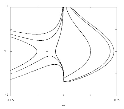
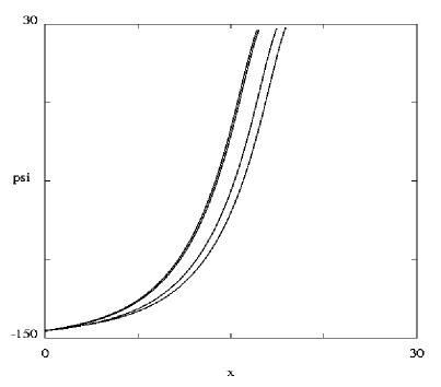
Figure 2.6: Numerical plots of the phase space in the $(w,v)$ coordinates, and the $\psi$ evolution with $x=log(t)$ for $n=\frac{1}{4}$. The ’$+$’ sign is a saddle point and the square is an unstable source.

At $n=\frac{1}{3}$ we are in the situation where the two critical points collapse into a unique one at the origin, creating a saddle-node bifurcation and a concomitant change in the behaviour and evolution of $\psi$. As $n$ keeps growing the single critical point splits into two critical points again. They move apart until the radiation value is reached, $n=\frac{1}{2}$ (Tr $M_{2}=0$). In this case, $\psi$ is a asymptotically monotonic growing function of time, with some small oscillations near the Planck epoch. However, note that in our universe the asymptote giving an increase of $\psi$ behaviour with time is never reached before the dust-dominated evolution takes over [107], [108], [109].

As the universe evolves to the dust-dominated epoch, and $n$ approaches the intermediate behaviour $n=\frac{3}{5}$, the two critical points start to coalesce again into a single point. When $n=\frac{3}{5}$ is reached, $\psi$ becomes a strictly monotonically growing function of time. When $n$ reaches the value corresponding to a dust-dominated universe, $n=\frac{2}{3}$, another saddle-node bifurcation occurs. The two critical points collapse into a single one. Again there will be change in the behaviour of $\psi$ for larger values of $n$. Accordingly, when $n>2/3,$ the two critical points reappear once again and $\psi$ becomes asymptotically constant in value.

Notice, that although a bifurcation is something that ’spoils’ the smooth behaviour of a system, in our case, that won’t happen, due to the physical constraints of our variables. In reality due to those constraints, the physical system will never ’feel’ the abrupt change at $n=\frac{1}{3}$ and $n=\frac{2}{3}$. This is also due to the fact that the attracting critical point always lies in the physical range of the variables, while the unstable one disappears form the physical system when the bifurcations occur, as can be seen from the phase plane plots.

Chapter 3 Gauge-Invariant Linear Perturbations of Varying-Alpha Cosmologies

Será este espelho a porta de entrada para a casa da verdade
em que ainda não fomos convidados?
– Ernesto Mota –

3.1 Introduction

In the previous chapter, using a phase space analysis of the equation of motion of the field $\psi$ (1.7.8), we have shown that BSBM theories have a number of appealing properties. They predict that, in a homogeneous and isotropic universe, there should be no variation of $\alpha$ during the radiation era and none during any present or late-time curvature or cosmological constant dominated era. During the dust era $\alpha$ should grow (leading to $\Delta\alpha/\alpha<0$ as observed) but only as $\log(t).$ Those results were also obtained by Barrow, Sandvik, and Magueijo [107, 108, 109, 110] using a different approach.

This behaviour allows the quasar data to be accommodated without producing conflict with recent geonuclear limits on allowed variations of $\alpha$, like the Oklo natural reactor limits of $\Delta\alpha/\alpha\lesssim 10^{-7}$ [20, 12, 11, 22, 8] because they are imposed at a very low effective redshift of $z\approx 0.15,$ at which time the universe has begun accelerating and all variations of $\alpha$ are damped out. Recent deductions of a possible upper limit of $\Delta\alpha/\alpha\lesssim 3\times 10^{-7}$ at $z=0.45$ from nuclear $\beta$ decays are potentially more restrictive [135, 25, 21]. These observations may be indeed problematic, since there is, at least, an order of magnitude difference between $\Delta\alpha/\alpha$ from the quasar data and the $\beta$-decay rate.

A possible approach to solve the discrepancy of the two results is to claim that one of the measurements has a non-identified problem which was not taken into account in the observations. However, it must be remembered that both the nuclear limits are derived from a local solar-system environment. In the absence of a theory relating the value of, and rate of change of, $\alpha$ on the cosmological scales where quasar lines form to their values in the virialised local inhomogeneities where galaxies, stars and planets form, one should be wary of ignoring the possible corrections that must be introduced when comparing planetary and quasar bounds: the density of the Earth would not, for example, be a good indicator of the density of the universe. Adding to that, we know that any varying-$\alpha$ theory implies the existence of a field, responsible for variations of $\alpha$, which is coupled to the matter fields. It is then natural, that strong variations of the density of matter in the universe, lead to spatial variations of $\psi$. Thus, inhomogeneity is an important factor in the study of varying-constant cosmological theories.

The first approach to address this problem, and the possibility of variations of $\alpha$ be influenced by matter inhomogeneities, is to consider the so called linear regime of the cosmological perturbations. In this regime, all the perturbations in the matter fields are very small. Much smaller than the background value of the fields.

In this chapter, we are then going to study the evolution of small, gauge-invariant perturbations to the exact Friedmann-Robertson-Walker solutions of the BSBM theory. The results of this investigation will reveal whether one must worry about fast growth of small initial inhomogeneities in the value of $\alpha$, which would lead to spatial variations of the value of the fine structure constant that might be more significant than the time variations at late times.

Our discussion is organised as follows. In section 2 of the we give the gauge-invariant perturbation equations following the development used in general relativity. In section 3 we specify the BSBM cosmology with varying $\alpha$ and derive the gauge invariant linear perturbation equations which couple the perturbations in the gravitational field to those in $\alpha$ and the density. In section 4 we solve for the time-evolution of small inhomogeneities in the fine structure constant on large and small scales for radiation, dust, and cosmological constant dominated expansion of the background universe. In section 5 we extend these studies into the non-linear regime by means of numerical solutions for flat and closed FRW universes. The evolution of spherical curvature inhomogeneities in density and in $\alpha$ is followed by computing the difference in time evolution between the FRW models of different curvature. These studies also reveal for the first time the behaviour of $\alpha$ in closed FRW models in the BSBM theory.

Units will be used in which $c=\hbar=1$; Greek indices run form $0$ to $3$ and Latin indices only over the spatial degrees of freedom $1$ to $3$. The Einstein summation convention is assumed; $a(t)$ is the scale factor of the background Friedmann-Robertson-Walker (FRW) metric and $G$ is Newton’s gravitation constant. Recall that in the BSBM varying-$\alpha$ theory, the quantities $c$ and $\hbar$ are taken to be constant, while $e$ varies as a function of a real scalar field $\psi,$ with $\alpha=e^{2},$ hence

$$e = e_{0}\exp[\psi]$$ (3.1.1)

$$\alpha = \alpha_{0}\exp[2\psi]$$ (3.1.2)

3.2 Linear Theory of Cosmological Perturbations

Observations indicate that the universe is nearly homogeneous and isotropic on large scales, in particular at early times where metric perturbations to the cosmic microwave background radiation are observed to be small $\approx 10^{-5}$ $<<1$. It is usually assumed that there exist small primordial perturbations which slowly increase in amplitude due to gravitational instability to form the structures we observe at the present time on the scales of galaxies and clusters of galaxies. The problem of describing the growth of small perturbations can be tackled using the cosmological perturbation theory, which is based on expanding the Einstein equations to linear order about the background metric. The theory was initially developed by Lifshitz [136], but many other approaches and improvements were done until today, see for instance [137, 138, 139, 140] for reviews.

Here we will follow the gauge invariant formalism developed in [141, 142] and we refer the reader to this references for more details in this particular approach. Also, we will a priori assume the existence of small inhomogeneities at some initial time in the early universe. Hence we will not discuss any particular model to create the primordial fluctuations in the matter fields, see [143, 144, 145, 146, 147] for different proposed models and hypothesis.

3.2.1 The background and metric perturbations

Assuming that the metric of spacetime deviates only by a small amount from a homogeneous, isotropic FRW spacetime, which is defined to be the background universe. It is convenient to split the metric into two parts: the first is the background metric, which represents the ideal background spacetime, and the second is its perturbation, which describes how the ’real’ spacetime deviates from the idealised background. This approach is mathematically well defined since it was shown in [148] that in the case of a FRW universe, solutions of the linearised field equations can be viewed as linearisations of solutions of the full non-linear ones.

The background line element is:

$$ds^{2}=^{(0)}g_{\mu\nu}dx^{\mu}dx^{\nu}=dt^{2}-a^{2}(t)\gamma_{ij}dx^{i}dx^{j}=a^{2}(\eta)(d\eta^{2}-\gamma_{ij}dx^{i}dx^{j}),$$ (3.2.1)

where $\eta$ is the conformal time,

$$d\eta=a^{-1}dt.$$

We choose the background metric to be the FRW metric, so

$$\gamma_{ij}=\delta_{ij}[1+\kappa(x^{2}+y^{2}+z^{2})]^{-2},$$

where $\kappa=0,1,-1$ depending on whether the three-dimensional hypersurfaces of constant $\eta$ are flat, closed or open. The Einstein equations are:

$$G_{\nu}^{\mu}=R_{\nu}^{\mu}-\frac{1}{2}\delta_{\nu}^{\mu}R=8\pi GT_{\nu}^{\mu},$$ (3.2.2)

where $R_{\nu}^{\mu}$ is the Ricci tensor, $R\equiv R_{\mu}^{\mu}$ is the Ricci scalar and $T_{\nu}^{\mu}$ is the total energy-momentum tensor. We shall exploit the fact that the BSBM theory for varying $\alpha$ can be expressed as general relativity with a particular linear combination of energy-momentum tensors. For the moment consider the presence of a single energy-momentum tensor. In the next section this will be decomposed appropriately.

For the background metric in equation (3.2.1), in conformal time, the Einstein equations reduce to the $0-0$ equation

$$\mathcal{H}^{2}=\frac{8\pi G}{3}a^{2}T_{0}^{0}-\kappa,$$ (3.2.3)

where $\mathcal{H}\equiv\frac{a^{\prime}}{a}$ using conformal time, and the $i-i$ equation:

$$\mathcal{H^{\prime}}+\mathcal{H}^{2}=\frac{4\pi G}{3}a^{2}T-\kappa,\qquad T\equiv T^{\mu}_{\mu}$$ (3.2.4)

For the background metric (3.2.1), the space-space part of the Ricci tensor $R_{j}^{i}$ is proportional to $\delta_{j}^{i}$. Thus, for an isotropic background universe, the energy-momentum tensor must also be spatially diagonal, $T_{j}^{i}\propto\delta_{j}^{i}$, in order that the Einstein equations are satisfied. Differentiating (3.2.3) with respect to $\eta$ and subtracting $2a^{\prime}$ we get the continuity equation for matter $\triangledown_{\mu}T_{0}^{\mu}=0$ :

$$dT^{0}_{0}=-(4T^{0}_{0}-T)d\ln{a}.$$ (3.2.5)

We now introduce small perturbations around the FRW background and follow the gauge-invariant approach of   Mukhanov et al [142]. The full line element may be expressed as:

$$ds^{2} = {}^{(0)}g_{\mu\nu}dx^{\mu}dx^{\nu}+\delta g_{\mu\nu}dx^{\mu}dx^{\nu},$$ (3.2.6)

where $\delta g_{\mu\nu}$ describes the perturbation. The full metric has been decoupled into its background parts and perturbation parts:

$$g_{\mu\nu} = {}^{(0)}g_{\mu\nu}+\delta g_{\mu\nu}.$$ (3.2.7)

The metric tensor has $10$ independent components in $4$ dimensions. For linear perturbations, the metric perturbation can be divided into three distinct types: scalar, vector and tensor, according to their transformation properties on spatial hypersurfaces [141, 149]. The reason for splitting the metric perturbation into these three types is that they are decoupled in the linear perturbations equations and so evolve independently. Neither of the vector and tensor perturbations exhibit growing instabilities in dust and radiation universes . Vector perturbations decay kinematically in an expanding universe whereas tensor perturbations lead to gravitational waves that do not couple to the isotropic energy-density and pressure inhomogeneities [142]. However, scalar perturbations may lead to growing inhomogeneities which, in turn, have an important effect on the dynamics of matter and thereby on the time and space variations of the fine structure constant in the BSBM theory. In this thesis we will then consider only the scalar perturbation modes.

It is shown in the literature, see for instance [141], that scalar perturbations can always be constructed from a scalar quantity, or its derivatives, and any background quantity, such as the $3$-metric $\gamma_{ij}$. We can then construct any first-order metric perturbation in terms of four scalars $\phi$, $\chi$, $B$ and $E$, which are functions of space and time coordinates [142]:

$$\delta g_{00} = -2a^{2}\phi,$$

$$\delta g_{0i} = \delta g_{i0}=a^{2}B_{|i},$$ (3.2.8)

$$\delta g_{ij} = -2a^{2}\left(\chi\gamma_{ij}-E_{|ij}\right)$$

where $|i$ represents the three-dimensional covariant derivative. The most general form of the scalar metric perturbations is then constructed using the four scalar quantities$\phi$, $\chi$, $B$ and $E$:

$\delta g_{\mu\nu}=\bordermatrix{&&\cr&2\phi&-B_{|i}\cr&-B_{|i}&2(\chi\gamma_{ij}-E_{|ij})\cr},$

From the above equation and equation (3.2.7), the line element for the background and for the scalar metric perturbations is

$$ds^{2}=a^{2}(\eta)\{(1+2\phi)d\eta^{2}-2B_{|i}dx^{i}d\eta-[(1-2\chi)\gamma_{ij}+2E_{|ij}]dx^{i}dx^{j})\}.$$ (3.2.9)

3.2.2 Gauge-invariant variables

The homogeneity of a FRW spacetime gives a natural choice of coordinates. But in the presence of first order perturbations we are free to make a first order change in the coordinates, that is, a gauge-transformation. This gauge freedom leads to several complications. For example, not all perturbed metrics correspond to perturbed spacetimes. It is possible to obtain an inhomogeneous form for the metric in a homogeneous and isotropic spacetime, by a choice of coordinates. Hence, it is important to be able to distinguish between physical inhomogeneities and mere coordinate artifacts.

The gauge problem of the cosmological perturbations is intimately related to the fact that we actually deal with two spacetimes, the physical space time, corresponding to the real universe and a fictitious one, which defines the unperturbed background. We need then to establish an one-to-one correspondence between the two spacetimes. For instance, when a coordinate system is introduced in the background we need to have a correspondent coordinate system in the real universe and vice-versa. This is necessary in order for us to be able to define a background spacetime into the real universe and to compare quantities between them. The need for that is clear from the definition of a perturbation in a given spacetime: a perturbation in a given quantity is the difference between its value at some event in the real spacetime and its value at the corresponding event in the background. This means that even if a quantity behaves as a scalar under coordinate transformations, its perturbation will not be invariant under gauge transformations. As a result we might end up with spurious gauge modes in the solutions, which have no meaning whatsoever.

There are two essential ways to deal with the gauge problem. The first is to choose a particular gauge and compute all the quantities in that gauge. If the gauge choice is well motivated, the perturbed variables will be easy to interpret. However, the task of selecting the best gauge for any given situation is not always trivial. See for example [136, 52] for more details on this approach. The second is to describe perturbations using gauge-invariant variables. We will follow here the second approach.

Gauge-invariant variables are unchanged under all infinitesimal scalar coordinate transformations, so they are independent of the background coordinates. Such quantities can be constructed out of the four scalar functions $\Phi$, $\Psi$, $E$ and $B$, see [141]. The simplest gauge-invariant linear combinations which span the space of gauge-invariant variables that can be constructed from the metric variables alone are [142]:

$$\Phi=\phi+\frac{[(B-E^{\prime})a]^{\prime}}{a},\qquad\Psi=\chi-\frac{a}{a^{\prime}}\left(B-E^{\prime}\right).$$ (3.2.10)

Note that any combination of gauge-invariant variables will also be gauge invariant. In general, a scalar quantity $f(\eta,\mathbf{{x})}$ defined in the spacetime can be split into its background value and a perturbation $f(\eta,)+\delta f(\eta,\mathbf{x})$. Since, in general, $\delta f$ is not gauge invariant, we cannot use this scalar quantity without modification if we want to have gauge-invariant equations. Hence, we consider the following gauge-invariant combination:

$$\delta f^{(gi)}=\delta f+f_{0}^{\prime}(B-E^{\prime}).$$ (3.2.11)

The freedom of gauge choice can be used to impose two conditions on the four scalar functions. The longitudinal gauge is defined by the conditions $E=B=0$. This gauge choice has the advantage of ruling out the complications of residual gauge modes. Also, in this gauge $\phi$ and $\chi$ coincide with the gauge-invariant variables $\Phi$ and $\Psi$ respectively. In this longitudinal gauge, the metric takes the form:

$$ds^{2}=a^{2}(\eta)[(1+2\Phi)d\eta^{2}-(1-2\Psi)\gamma_{ij}dx^{i}dx^{j})],$$

and the gauge invariants $\Phi$ and $\Psi$ become the amplitudes of the metric perturbations in the longitudinal coordinate system. In the case where there are no space-space components in the energy-momentum tensor, so $T_{j}^{i}\propto\delta_{j}^{i}$, we have that $\Phi=\Psi$ and there remains only one free metric perturbation variable which is a generalisation of the Newtonian gravitational potential. As can be seen from the above equation, the gauge invariants $\Phi$ and $\Psi$ have a simple physical interpretation: they are the amplitudes of the metric perturbations in the longitudinal coordinate system.

3.2.3 The linearly perturbed Einstein equations

For small perturbations of the metric, the Einstein tensor can be written as $G_{\nu}^{\mu}=\ ^{(0)}G_{\nu}^{\mu}+\delta G_{\nu}^{\mu}$, and the energy-momentum tensor can be split in a similar way. The fully perturbed Einstein equations can be obtained for scalar perturbation modes with the line element given by (3.2.9). However, these equations are not gauge invariant, since they contain non gauge-invariant quantities. In order to have gauge-invariant equations we need to replace $\phi$ and $\chi$ by the gauge-invariant variables $\Phi$, $\Psi$ and $B-E^{\prime}$, and to construct the gauge-invariant equivalents of $\delta G_{\nu}^{\mu}$ and $\delta T_{\nu}^{\mu}$, we need to rewrite then as [142]:

$$\delta G_{0}^{(gi)\ 0} = \delta G_{0}^{0}+(^{(0)}G_{0}^{0})^{\prime}(B-E^{\prime}),$$

$$\delta G_{j}^{(gi)\ i} = \delta G_{j}^{i}+(^{(0)}G_{j}^{i})^{\prime}(B-E^{\prime}),$$ (3.2.12)

$$\delta G_{i}^{(gi)\ 0} = \delta G_{i}^{0}+(^{(0)}G_{0}^{0}-\frac{1}{3}\ ^{(0)}G_{k}^{k})(B-E^{\prime})_{|i},$$

and analogously for $\delta T_{\nu}^{\mu}$,

$$\delta T_{0}^{(gi)\ 0} = \delta T_{0}^{0}+(^{(0)}T_{0}^{0})^{\prime}(B-E^{\prime}),$$ (3.2.13)

$$\delta T_{j}^{(gi)\ i} = \delta T_{j}^{i}+(^{(0)}T_{j}^{i})^{\prime}(B-E^{\prime}),$$ (3.2.14)

$$\delta T_{i}^{(gi)\ 0} = \delta T_{i}^{0}+(^{(0)}T_{0}^{0}-\frac{1}{3}\ ^{(0)}T_{k}^{k})(B-E^{\prime})_{|i}.$$ (3.2.15)

The components of the perturbed Einstein equations linearised around small perturbations of the background are $\delta G_{\nu}^{(gi)\ \mu}=8\pi G\delta T_{\nu}^{(gi)\ \mu}$:

$$\delta G_{0}^{0} = \triangledown^{2}\Phi-3\mathcal{H}\Phi^{\prime}-3\Phi(\mathcal{H}^{2}-\kappa)=4\pi Ga^{2}\delta T_{0}^{(gi)0}$$

$$\delta G_{i}^{0} = \partial_{i}(a\Phi)^{{}^{\prime}}=4\pi Ga\delta T_{i}^{(gi)0}$$ (3.2.16)

$$\delta G_{i}^{j} = \Phi^{\prime\prime}+3\mathcal{H}\Phi^{\prime}+\Phi(2\mathcal{H}^{\prime}+\mathcal{H}^{2}-\kappa)=-4\pi Ga^{2}\delta T_{j}^{(gi)i}$$

where we have already simplified the equations since the energy-momentum tensor that we will be considering in section 3 has no space-space components and so $\Phi=\Psi$.

In order to close our system of equations, we need equations of motion for the matter formulated in a gauge-invariant way. This requires explicit expressions for the energy-momentum tensor and so we must now specify the BSBM theory.

3.3 Cosmological Perturbations and the BSBM Model

It was shown in chapter 1 that, in the context of the BSBM model, the homogeneous evolution of $\psi$ does not create significant metric perturbations at late times and the cosmological time-evolution of the expansion scale-factor is very well approximated by the usual power-laws found in $\kappa=0$ FRW models filled with a perfect fluid (see also[110] ).

Therefore, we will assume there are no major modifications in the perturbed spacetime which would lead to changes of the behaviour of the perturbed variables of a perturbed FRW spacetime filled with perfect fluid. That is, we will assume that the energy-density perturbations and the metric potential are the same as in a FRW universe with no variation of $\alpha$. Physically, this is to be expected for most of the evolution, although this assumption might break down (along with much else) on approach to initial and final cosmological singularities. It is a reflection of the fact that the changes in $\alpha$ have negligible feedback into the changes in the expansion, which are governed to leading order by gravity. The principal effects are those of perturbations in the matter density and expansion rate on the evolution of $\alpha.$ This simplification will allow us to write the time and space variations of the scalar field, $\delta\psi$, as a functions of $\rho_{m}$, $\rho_{r}$, $\delta\rho_{m}$, $\delta\rho_{r}$ , $\Phi$ and $\psi$, where $\delta\rho_{m}$, $\delta\rho_{r}$ and $\Phi$ will be given by the solutions found in ref. [142] for universes with no variation of $\alpha;$ the field $\psi$ will be given by the solutions found previously in chapter 2. In order to find an expression for $\delta\psi$ in terms of these quantities we need to write the gauge-invariant linearly perturbed Einstein equations for the BSBM model.

3.3.1 The background equations

We vary the action (1.7.2) with respect to the metric to obtain the generalised Einstein equations:

$$G_{\nu}^{\ \mu}=8\pi G\left(T_{\nu}^{\mathit{matter}\ \mu}+T_{\nu}^{\psi\ \mu}+T_{\nu}^{\mathit{em}\ \mu}\right)$$

where $T_{\mu\nu}^{\mathrm{mat}}=\frac{2}{\sqrt{-g}}\frac{\delta(\sqrt{-g}\mathcal{L}_{\mathrm{mat}})}{\delta g^{\mu\nu}}$ is the energy-momentum tensor for perfect-fluid matter fields, and

$$T_{\mu\nu}^{\mathrm{matter}}=(\rho_{m}+p_{m})u_{\mu}u_{\nu}-p_{m}g_{\mu\nu},$$

where $u^{\mu}$ $=\delta_{0}^{\mu}$ is the comoving fluid 4-velocity; $T_{\nu}^{\psi\ \mu}$ and $T_{\nu}^{\mathit{em}\ \mu}$ are the energy-momentum tensors for the kinetic energy of the field $\psi$ and the electromagnetic field respectively:

$$T_{\mu\nu}^{\psi}=\omega\partial_{\mu}\psi\partial_{\nu}\psi-{\frac{\omega}{2}}g_{\mu\nu}\partial_{\beta}\psi\partial^{\beta}\psi,\quad T_{\mu\nu}^{\mathrm{em}}=F_{\mu\beta}F_{\nu}^{\beta}e^{-2\psi}-{\frac{1}{4}}g_{\mu\nu}F_{\sigma\beta}F^{\sigma\beta}e^{-2\psi}.$$

Note, the total energy density of the electromagnetic field is the sum of the Coulomb energy density $\zeta\rho_{m}$ and the radiation energy density $\rho_{r}$ , where $-1\leq\zeta\leq 1$ is the fraction of mass density $\rho_{m}$ of matter in the form of the Coulomb energy. We will then consider $T_{\nu}^{\mathit{em}\ \mu}$ as a perfect fluid:

$$T_{\mu\nu}^{\mathrm{em}}=(|\zeta|\rho_{m}+\rho_{r}+p_{m}+p_{r})e^{-2\psi}u_{\mu}u_{\nu}-\left(p_{m}+p_{r}\right)e^{-2\psi}g_{\mu\nu}$$

The propagation equation for $\psi$ comes from the variational principle as:

$${\partial_{\mu}\left[\sqrt{-g}g^{\mu\nu}\partial_{\nu}\psi\right]=-\frac{2}{\omega}}\sqrt{-g}e^{-2\psi}\mathcal{L}_{\mathrm{em}}.$$ (3.3.1)

This equation determines how $e,$ and hence $\alpha$, varies with time.

The background equations can now be explicitly obtained:

$$3{{\mathcal{H}}^{2}} = 8\pi Ga^{2}\left(\rho_{m}+\left(\rho_{r}+|\zeta|\rho_{m}\right)e^{-2\psi}+\frac{\omega}{2}a^{-2}{{\psi^{\prime}}^{2}}\right)+a^{2}\Lambda-3\kappa$$ (3.3.2)

$$3{\mathcal{H^{\prime}}} = -4\pi Ga^{2}\left(\rho_{m}\left(1+|\zeta|e^{-2\psi}\right)+2\rho_{r}e^{-2\psi}+2\omega a^{-2}{{\psi^{\prime}}^{2}}\right)+a^{2}\Lambda$$

where $\Lambda$ is the cosmological constant. The equation of motion for the $\psi$ field is:

$$2\mathcal{H}\psi^{\prime}+\psi^{\prime\prime}=\frac{2|\zeta|{{a}^{2}}}{\omega}\rho_{m}e^{-2\psi}$$ (3.3.3)

The conservation equations for the matter fields, $\rho_{r}$ and $\rho_{m}$ respectively, are:

$$\rho_{m}^{\prime}+3{\mathcal{H}}\rho_{m} = 0$$ (3.3.4)

$$\rho_{r}^{\prime}+4{\mathcal{H}}\rho_{r}^{\prime} = 2\psi^{\prime}\rho_{r}.$$ (3.3.5)

3.3.2 Linear perturbations in the BSBM theory

The perturbed components of the total energy-momentum ($T_{\mu\nu}^{total}=T_{\mu\nu}^{mat}+T_{\mu\nu}^{\psi}+T_{\mu\nu}^{em}$) arise from perturbations of the different matter fields which are time and space dependent. In particular, we have $\rho_{m}\rightarrow\rho_{m}+\delta\rho_{m}$, $\rho_{r}\rightarrow\rho_{r}+\delta\rho_{r}$ and $\psi\rightarrow\psi+\delta\psi$. Note also that we have to perturb the fluid 4-velocity field, so we have $u_{i}\rightarrow u_{i}+\delta u_{i}$, where $i$ $=1,2,3$.

In order to have gauge-invariant equations we need to express the perturbed energy-momentum tensor in terms of the gauge-invariant energy density, pressure, scalar field and velocity field perturbations . The gauge invariants $\delta\rho_{m}^{(gi)}$, $\delta\rho_{r}^{(gi)}$ and $\delta\psi^{(gi)}$ are defined in the same way as the gauge-invariant perturbation of a general four-scalar, see equation (3.2.10), so:

$$\delta\rho_{m}^{(gi)}=\delta\rho_{m}+\rho_{m}^{\prime}(B-E^{\prime}),\quad\delta p^{(gi)}=\delta p+p^{\prime}(B-E^{\prime}),\quad\delta\psi^{(gi)}=\delta\psi+\psi^{\prime}(B-E^{\prime}),$$

where $\delta p$ is the perturbed pressure for a specific component and the gauge-invariant three-velocity $\delta u_{i}^{(gi)}$ is given by [142]:

$$\delta u_{i}^{(gi)}=\delta u_{i}+a(B-E^{\prime})_{|i}.$$

The physical meaning of the quantities which enter the gauge-invariant equations is very simple: they coincide with the corresponding perturbations in the longitudinal gauge. From now on we will drop the superscript $(gi)$ since we will always be dealing only with gauge-invariant quantities.

We can now write the gauge-invariant linearly perturbed energy-momentum tensor:

$$\delta T_{0}^{\mathit{matter}\ 0} = \delta\rho_{m},$$ (3.3.6)

$$\delta T_{i}^{\mathit{matter}\ 0} = \left(\rho_{m}+p_{m}\right)a^{-1}\delta u_{i},$$ (3.3.7)

$$\delta T_{j}^{\mathit{matter}\ i} = -\delta p_{m}\delta_{j}^{i},$$ (3.3.8)

$$\delta T_{0}^{\psi\ 0} = \omega a^{-2}\left(\psi^{\prime}\delta\psi^{\prime}-\psi^{{\prime}^{2}}\Phi\right),$$ (3.3.9)

$$\delta T_{i}^{\psi\ 0} = \omega a^{-2}\psi^{\prime}\partial_{i}\delta\psi,$$ (3.3.10)

$$\delta T_{j}^{\psi\ i} = \omega a^{-2}\left(\psi^{{\prime}^{2}}\Phi-\psi^{\prime}\delta\psi^{\prime}\right)\delta_{j}^{i},$$ (3.3.11)

$$\delta T_{0}^{\mathit{em}\ 0} = \left(|\zeta|\delta\rho_{m}+\delta\rho_{r}\right)e^{-2\psi}-2e^{-2\psi}\left(|\zeta|\rho_{m}+\rho_{r}\right)\delta\psi,$$ (3.3.12)

$$\delta T_{i}^{\mathit{em}\ 0} = e^{-2\psi}\left(|\zeta|\rho_{m}+\rho_{r}+p_{m}+p_{r}\right)a^{-1}\delta u_{i},$$ (3.3.13)

$$\delta T_{j}^{\mathit{em}\ i} = \left(2\delta\psi\left(p_{m}+p_{r}\right)e^{-2\psi}-\left(\delta p_{m}+\delta p_{r}\right)e^{-2\psi}\right)\delta_{j}^{i}.$$ (3.3.14)

We have assumed there are no anisotropic stresses in the energy-momentum tensors and we have considered only adiabatic perturbations; that is, we consider the pressure perturbations to depend only on the energy-density perturbations. In the dust and radiation cases this means $p_{m}=0$, $\delta p_{m}=0$, or $p_{r}=\frac{1}{3}\rho_{r}$ and $\delta p_{r}=\frac{1}{3}\rho_{r}$, respectively.

The fully perturbed gauge–invariant Einstein equations can be obtained from (3.2.3) using the expressions above for $\delta T_{\nu}^{\mu}$ ( 3.3.6-3.3.14). We have

$$\Phi\left(-3\mathcal{H}^{2}+3k+4G\pi\omega{\psi^{\prime}}^{2}\right)+\triangledown^{2}\Phi-4G\pi\omega\psi^{\prime}\delta\psi^{\prime}-3\mathcal{H}\Phi^{\prime}=$$

$$4G\pi{a}^{2}e^{-2\psi}\left[\left(e^{2\psi}+|\zeta|\right)\delta\rho_{m}+\delta\rho_{r}-2\delta\psi\left(\rho_{r}+|\zeta|\rho_{m}\right)\right]$$ (3.3.15)

$$\mathcal{H}\triangledown^{2}\Phi+\triangledown^{2}\Phi^{\prime}=\\ 4G\pi\omega\psi^{\prime}\triangledown^{2}\delta\psi-\frac{4G\pi}{3}ae^{-2\psi}\left[4\rho_{r}+3\left(e^{2\psi}+|\zeta|\right)\rho_{m}\right]\triangledown\delta u$$

$$\Phi\left({\mathcal{H}}^{2}+2\mathcal{H}^{\prime}-k+4G\pi\omega{\psi^{\prime}}^{2}\right)+3\mathcal{H}\Phi^{\prime}+\Phi^{\prime\prime}=$$

$$\frac{4G\pi}{3}\left[{a}^{2}e^{-2\psi}\left(\delta\rho_{r}-2\rho_{r}\delta\psi\right)+3\omega\psi^{\prime}\delta\psi^{\prime}\right]$$ (3.3.16)

It is useful to write the perturbed energy-momentum conservation equations for each component:

$$\delta\psi^{{}^{\prime\prime}}=\frac{2|\zeta|}{\omega}e^{-2\psi}{a}^{2}\left[\delta\rho_{m}+2\rho_{m}\left(\Phi-\delta\psi\right)\right]-2\mathcal{H}\delta\psi^{{}^{\prime}}+\triangledown^{2}\delta\psi+4\psi^{\prime}\Phi^{{}^{\prime}},$$ (3.3.17)

$$\delta\rho_{r}^{{}^{\prime}}=-\frac{2}{3}\left[\delta\rho_{r}\left(6\mathcal{H}-3\psi^{\prime}\right)+\rho_{r}\left(2\triangledown\delta u-3\delta\psi^{{}^{\prime}}-6\Phi^{{}^{\prime}}\right)\right],$$ (3.3.18)

$$\delta\rho_{m}^{{}^{\prime}}=-3\mathcal{H}\delta\rho_{m}-\rho_{m}\left(\triangledown\delta u-3\Phi^{{}^{\prime}}\right).$$ (3.3.19)

From these expressions it is clear that perturbations in $\alpha$ are sourced by perturbations in the dust, but not vice versa. Hence we expect that, in a dust-dominated universe with varying $\alpha$, the cold dark matter perturbations will behave as in a dust-dominated universe with no varying $\alpha$. Notice however that the same cannot be concluded so easily for a radiation-dominated era, since there is a source term in equation (3.3.18) proportional to $\delta\psi^{\prime}$. We expect this term to be negligible at large scales, but that might not be the case on small scales.

The gauge-invariant perturbation for $\alpha$ is given by equation (3.1.1) as

$$\frac{\delta\alpha}{\alpha}=2\delta\psi.$$

From equations (3.3.2), (3.3.2), (3.3.2), using (3.3.2) to simplify, we obtain the general form for $\delta\psi,$ the perturbation to the scalar field which drives variations of the fine structure constant, as

$$\delta\psi = \frac{1}{8G\pi{a}^{2}\left(2\rho_{r}+3|\zeta|\rho_{m}\right)}\left(4G\pi{a}^{2}\left[2\left(\delta\rho_{r}-4\rho_{r}\Phi\right)+3\left(e^{2\psi}+|\zeta|\right)\right.\right.$$

$$\left.\left.\left(\delta\rho_{m}-2\rho_{m}\Phi\right)\right]+3e^{2\psi}\left[2\Phi\left(3\mathcal{H}^{2}-k-4G\pi\omega{\psi^{\prime}}^{2}\right)-\triangledown^{2}\Phi+6\mathcal{H}\Phi^{{}^{\prime}}+\Phi^{{}^{\prime\prime}}\right]\right)$$

This is a gauge-invariant expression for $\delta\psi$, written as a function of the gauge-invariant quantities $\Phi$, $\delta\rho_{m}$, and $\delta\rho_{r}$.

3.4 Evolution of the Perturbations

In a spatially flat universe, $\kappa=0$, the general gauge-invariant expression for $\delta\psi$ becomes:

$$\delta\psi = \frac{1}{8G\pi{a}^{2}\left(2\rho_{r}+3|\zeta|\rho_{m}\right)}\left(4G\pi{a}^{2}\left[2\left(\delta\rho_{r}-4\rho_{r}\Phi\right)+3\left(e^{2\psi}+|\zeta|\right)\right.\right.$$

$$\left.\left.\left(\delta\rho_{m}-2\rho_{m}\Phi\right)\right]+3e^{2\psi}\left[\Phi\left(6\mathcal{H}^{2}-8G\pi\omega{\psi^{\prime}}^{2}\right)-\triangledown^{2}\Phi+6\mathcal{H}\Phi^{{}^{\prime}}+\Phi^{{}^{\prime\prime}}\right]\right).$$

It was shown in chapter 2 that the cosmological evolution of the metric scale factor is unchanged (up to very small logarithmic corrections) to leading order by the time evolution of $\psi$. The dominant effect is that of the evolution of the scale factor on the evolution of $\psi$ through its propagation equation.

It is known that perturbations of massless scalar fields, or scalar fields with a very small mass are negligible with respect to perturbations in the matter fields and the gravitational potential. Guided by this, in order to obtain the evolutionary behaviour for $\frac{\delta\alpha}{\alpha}$, we will assume that the matter field perturbations, $\delta\rho_{m}$ and $\delta\rho_{r}$, and the metric perturbations, $\Phi$, are unaffected by the $\psi$ perturbations to leading order. We will assume that these three quantities will therefore be the same to this order as they are in a flat FRW universe filled with barotropic matter and a minimally coupled scalar field. These assumptions are valid if the energy density of $\psi$ is much smaller than the energy density of the matter fields, so $\Phi$ will be driven only by the matter perturbations. If we examine the perturbations in the non-linear regime it is confirmed that $\frac{\delta\psi}{\psi}\ll\frac{\delta\rho}{\rho}$ (see figure (3.4)). 

3.4.1 Radiation-dominated universes

In any radiation-dominated era in which the expansion of the universe is dominated by relativistic particles with an equation of state $p=\frac{1}{3}\rho$, we can neglect the non-relativistic stresses in the universe, in particular, the cold dark matter and the cosmological constant since $\rho_{r}>>\rho_{m}>>\rho_{\Lambda}$ to a good approximation. If we assume that $\rho_{\Lambda}=\rho_{\Lambda}=0=\kappa$ and $\delta\rho_{m}=0$, the background equations of motion give the usual conformal time evolution for the scale factor and the energy density of the radiation:

$$\rho_{r}=\rho_{r_{0}}a^{-4}e^{2\psi}\qquad a=\sqrt{8\pi G\rho_{r_{0}}}\eta$$

where $\rho_{r_{0}}$ is a constant.

The perturbations in the barotropic matter fluid and the potential $\Phi$ come from the equations (3.3.2), (3.3.2). The usual flat FRW solutions with constant $\alpha$ are obtained by setting the terms proportional to $\psi$ to zero, (3.3.2). The general solution of these equations can be obtained by expanding the physical quantities in terms of the eigenfunctions of the operator $\triangledown^{2}$ (where $-k^{2}$ denotes the eigenvalue of this operator) and solving for each mode separately. Resuming the terms, the general solutions of the linearly perturbed equations for the potential $\Phi$ and the barotropic matter are:

$$\Phi=\eta^{-3}\{\left[w\eta\cos(w\eta)-\sin(w\eta)\right]C_{1}+\left[w\eta\sin(w\eta)+\cos(w\eta)\right]C_{2}\}e^{i\mathbf{kx}}$$ (3.4.2)

and

$$\frac{{\delta\rho_{r}}}{\rho_{r}} = \frac{4}{\eta^{3}}\left(C_{1}\{\eta w\left[1-\frac{1}{2}\left(\eta w\right)^{2}\right]\cos(\eta w)+\left[\left(\eta w\right)^{2}-1\right]\sin(\eta w)\}\right.$$

$$+\{\left[1-\left(\eta w\right)^{2}\right]\cos(\eta w)+\eta w\left[1-\frac{1}{2}\left(\eta w\right)^{2}\right]\sin(\eta w)\}C_{2})e^{i\mathbf{kx}},$$

where we have expanded the general solution in plane waves since we are assuming a spatially flat universe; $C_{1}$ and $C_{2}$ are arbitrary functions of the spatial coordinates; $k$ is the wave vector mode and $w=k/\sqrt{3}$. Note that these quantities are all expressed in their gauge-invariant format. Finally, to calculate the explicit time dependence of $\delta\psi$, we need to use the background solution for $\psi$:

$$\psi=\frac{1}{2}\log{(8N)}+\frac{1}{4}\log{(\frac{a_{0}}{2}\eta^{2}).}$$ (3.4.4)

This was found in chapter 2 and [109, 1] for a radiation-dominated universe, where $N=-\frac{2\zeta}{\omega}\rho_{m}a^{3}>0$ since $\zeta<0$ in the magnetic energy dominated theories considered by BSBM. It is important to notice that in universes with an entropy to baryon ratio ($S\sim 10^{9}$) like our own, $\psi$ does not experience any growth in time [108]. The constant term on the right-hand side of (3.4.4) dominates the solution for $\psi(\eta)$ throughout the radiation era. Numerical solutions confirm this freezing in of $\psi$, and hence of $\alpha$, during the radiation era, [107].

Large-scale perturbations in a radiation-dominated era

In the long-wavelength limit ($w\eta<<1$) where the scale of the perturbation exceeds the Hubble radius, we can neglect spatial gradients. So, in this limit, $\frac{\delta\alpha}{\alpha}$ becomes:

$$\delta\psi=\frac{1}{2}\frac{\delta\alpha}{\alpha}\propto\frac{1}{2\eta}e^{i\mathbf{kx}}\triangledown^{2}C_{2}-4\pi Gwe^{i\mathbf{kx}}C_{2}\eta^{-3}$$

From this expression we can see at that on large scales the inhomogeneous perturbations in $\alpha$ will decrease as a power-law in time. This behaviour agrees with the one found in [110] by other methods.

Small-scale perturbations in a radiation-dominated era

On scales smaller than the Hubble radius ($w\eta>>1$) the dominant terms are proportional to $\triangledown^{2}C_{1}$ and $\triangledown^{2}C_{2}$, so the asymptotic behaviour for $\frac{\delta\alpha}{\alpha}$ will be:  

$$\delta\psi = \frac{1}{2}\frac{\delta\alpha}{\alpha}\propto-\frac{1}{2}w\left[\cos(\eta w)\triangledown^{2}C_{1}+\sin(\eta w)\triangledown^{2}C_{2}\right]e^{i\mathbf{kx}}+$$

$$+\frac{1}{2\eta}\left[\sin(\eta w)\triangledown^{2}C_{1}-\cos(\eta w)\triangledown^{2}C_{2}\right]e^{i\mathbf{kx}}$$

On small scales we can see the perturbations on $\alpha$ will be oscillatory. This behaviour is new and does not coincide with the ones found in [110].

In reality, we expect dissipation of the adiabatic fluctuations to occur by Silk damping [150] and small-scale fluctuations in $\alpha$ will also undergo decay as their driving terms damp out. However, while the exact solution for the evolution of $\alpha$ is a linear sum of a constant and a slow power-law growth, the power-law evolution does not become dominant by the end of the radiation era in universes like our own with entropy per baryon $O(10^{9}).$

3.4.2 Dust-dominated universes

In the case of a flat dust-dominated universe, filled with a $p=0$ fluid, we can assume $\rho_{r}=\rho_{\Lambda}=0=\kappa$ and $\delta\rho_{r}=0$. Again, in order to obtain an explicit expression of $\delta\psi$ from equation (3.4), we will assume that the matter-field perturbations, $\rho_{m}$ and $\delta\rho_{m}$, and the metric perturbation, $\Phi$, are not affected by the $\psi$ perturbations to leading order. Thus, we will assume that these functions behave as in a perturbed flat FRW dust universe.

In general, for a flat dust universe we have the following background solutions:

$$\rho_{m}=\rho_{m_{0}}a^{-3},\qquad a=\frac{2\pi G\rho_{m_{0}}}{3}\eta^{2},$$

where $\rho_{m_{0}}$ is constant.

As before, we can calculate the most general gauge-invariant solutions for the energy-momentum perturbations $\delta\rho_{m},$ and for the potential $\Phi$, assuming that the $\psi$ field does not affect them to leading order, so their time dependences are [142]:

$$\Phi=C_{1}+C_{2}\eta^{-5}$$ (3.4.6)

and

$$\frac{\delta\rho_{m}}{\rho_{m}}=\frac{1}{6}\left[\left(\eta^{2}\triangledown^{2}C_{1}-12C_{1}\right)+\left(\eta^{2}\triangledown^{2}C_{2}+18C_{2}\right)\eta^{-5}\right],$$ (3.4.7)

where $C_{1}$ and $C_{2}$ are arbitrary functions of the spatial coordinates.

Once again, we need the background solution for $\psi$, in order to calculate $\delta\psi$ as an explicit function of the conformal time. We use the asymptotic solution

$$\psi=\frac{1}{2}\log{[2N\log{(\frac{a_{m}}{6}\eta^{3})}],}$$

which was found in [110], as an asymptotic approximation for a dust-dominated universe which is in good agreement with numerical solutions, and where, as above, $N=-\frac{2\zeta}{\omega}\rho_{m}a^{3}>0$ is a constant.

Large-scale perturbations in a dust-dominated era

On scales larger than the Hubble radius we can neglect the terms proportional to $\partial_{i}C_{1}$,$\triangledown^{2}C_{1}$, $\triangledown^{2}C_{2}$ and $\partial_{i}C_{2}$; so in this limit we have the following asymptotic behaviour for the non-decaying mode:

$$\delta\psi=\frac{1}{2}\frac{\delta\alpha}{\alpha}\propto-2C_{1}-\frac{2\pi G\rho_{m_{0}}}{\ln(\eta)}C_{1}$$ (3.4.8)

Therefore, on large scales the inhomogeneous perturbations of $\alpha$ will not grow in time by gravitational instability. This behaviour can be understood with reference to the general evolution equation for $\psi$ in Friedmann universes. On large scales, where spatial gradients in $\psi$ can be neglected with respect to its time derivatives, we may view inhomogeneities in density and in $\psi$ as if they are separate Friedmann universes of non-zero curvature ($\kappa\neq 0$). The growth of inhomogeneity can be deduced by comparing the evolution of $\alpha$ in the $\kappa\neq 0$ universes with those in the $\kappa=0$ model (a more detailed numerical study of this model will be presented in section 5 below). In effect, this uses the Birkhoff-Newton property of gravitational fields with spherical symmetry [151]. We note that the (3.3.3) evolution equation has the simple property that $\psi$ cannot have a maximum because $\ddot{\psi}>0$ when $\dot{\psi}>0$ because $N>0$ , [110]. This result holds irrespective of the value of $\kappa\lesseqqgtr 0.$ Thus $\psi$ and $\alpha$ will continue their slow increase in both over-densities, under-densities and the flat background until we reach scales small enough for spatial derivative to come significantly into play. This has the important consequence that we do not expect large spatial inhomogeneities in $\alpha$ to have developed. However, it should be noted that the sensitivity of the observations of varying-$\alpha$ effects in quasar spectra is sufficient to discern variations of redshift space smaller than $O(10^{-5})$, which is of the same order as the amplitude of density fluctuation on very large scales in the universe.  

Small-scale perturbations in a dust-dominated era

On scales smaller than the Hubble radius the dominant terms are those proportional to $\triangledown^{2}C_{1}$ and $\triangledown^{2}C_{2}$, so the asymptotic behaviour for the growing mode will be:

$$\delta\psi\propto\frac{1}{12}\eta^{2}\triangledown^{2}C_{1}$$ (3.4.9)

This shows that perturbations of $\alpha$ will grow on small scales. This result is a product of the assumption that on small scales the universe can be considered as being filled by an homogeneous and isotropic fluid, however we know this is not true below the scale where gravitational clustering becomes non-linear. On these small scales we also have to worry about new consequences of inhomogeneity which have not been included in our analysis. For example, the constant parameter $N=-\frac{2\zeta}{\omega}_{m}a^{3}\varpropto\zeta\Omega_{m}$ will vary in space due to inhomogeneity in the background matter density parameter $\Omega_{m}$ and in the dark matter parameter $-1\leq\zeta\leq 1$. We have assumed that $\zeta<0$ for the cold dark matter on large scales in order for the cosmological consequences of time-varying $\alpha$ to be a small perturbation to the standard cosmological dynamics. But on small scales the dark matter will be baryonic in nature and so $\zeta>0$ there. Hence, we expect $\zeta$ to be significantly scale dependent as we go to small scales.

3.4.3 Accelerated expansion

In an era of accelerated expansion, $\ddot{a}>0$, as would arise during inflation or during a $\Lambda$- or quintessence-dominated epoch at late times, we can consider the scale factor to evolve as a power-law of the conformal time as $a=\eta^{-n}$, where $n\geq 1$ and $\eta$   runs from $-\infty$ to $0$. The case of $a=\eta^{-1}$ corresponds to a $\Lambda$ -dominated epoch.

As in the previous sections, we will assume that all the other matter components which fill the universe will behave exactly as in a perturbed FRW universe with no variations of $\alpha$. We also assume that neither of the dust and radiation perturbations will affect the behaviour and evolution of $\delta\psi$, and that these perturbations are negligible with respect to the $\Lambda$ stress driving the expansion, so we will consider $\delta\rho_{m}=0$ and $\delta\rho_{r}=0$.

We saw in chapter 2, that a universe which is undergoing accelerated expansion, the asymptotic solution for $\psi$ is a constant, so we will assume that $\psi=\psi_{\infty}$, in the background, where $\psi_{\infty}$ is a constant. Thus, equations (3.3.2) and (3.3.2) become:

$$\frac{8G\pi|\zeta|\delta\psi\rho_{m}}{e^{2\psi_{\infty}}\eta^{2n}}+\triangledown^{2}\Phi+\frac{3n\left(\eta\Phi-n\Phi^{{}^{\prime}}\right)}{\eta^{2}}=0$$

$$n\left(2+n\right)\Phi+\eta\left(\eta\Phi^{{}^{\prime\prime}}-3n\Phi^{{}^{\prime}}\right)=0$$

where we have also considered $\rho_{r}=0$, but $\rho_{m}\neq 0$ because of the coupling with $\psi$ in the equation of motion of the scalar field. Note that if we had also set $\rho_{m}=0$ here, we would have imposed a no $\alpha$-variation condition: $\delta\psi=0$.

Integrating the last equation, we obtain

$$\Phi=\eta^{\frac{3n-\sqrt{1+n\left(5n-2\right)}}{2}}\left(\sqrt{\eta}C_{1}+\eta^{\frac{1}{2}+\sqrt{1+n\left(5n-2\right)}}C_{2}\right)$$

where $C_{1}$ and $C_{2}$ are arbitrary functions of the spatial coordinates. Note that since $n>1$ in accelerating universes we see that $\Phi$ will decay in time as $\eta\rightarrow 0$. From this solution for $\Phi$, we obtain:

$$\delta\psi = \frac{1}{2}\frac{\delta\alpha}{\alpha}=-\frac{e^{2\psi_{\infty}}}{16G\rho_{m_{0}}\pi|\zeta|}\eta^{\frac{-3+n-\sqrt{1+n\left(-2+5n\right)}}{2}}\left[3n\left(1+n-\sqrt{1+n\left(5n-2\right)}\right)C_{1}+\right.$$

$$\left.3n\left(1+n+\sqrt{1+n\left(5n-2\right)}\right)\eta^{\sqrt{1+n\left(5n-2\right)}}C_{2}+2\eta^{2}\triangledown^{2}C_{1}+2\eta^{2+\sqrt{1+n\left(5n-2\right)}}\triangledown^{2}C_{2}\right]$$

which is a decaying function of the conformal time when $n>1$ and a constant when $n=1$. Thus, in accord with the expectations of the cosmic no hair theorem, the universe approaches the FRW model and $\alpha$ is asymptotically constant at late times [152].

Large-scale perturbations during accelerated expansion

On scales larger than the Hubble radius we can neglect the terms proportional to the spatial derivatives; so in this limit we have the following asymptotic behaviour:

$$\delta\psi \propto -\frac{3e^{2\psi_{\infty}}n}{16G\rho_{m_{0}}\pi|\zeta|}\eta^{\frac{n-3-\sqrt{1+n\left(5n-2\right)}}{2}}\left[\left(1+n-\sqrt{1+n\left(5n-2\right)}\right)C_{1}\right.$$ (3.4.10)

$$\left.+\left(1+n+\sqrt{1+n\left(5n-2\right)}\right)\eta^{\sqrt{1+n\left(5n-2\right)}}C_{2}\right]$$

Therefore, as expected, on large scales during an accelerated era inhomogeneities in $\alpha$ will decrease on time when $n>1$ and will be a constant when $n=1$.

Small-scale perturbations during accelerated expansion

On scales smaller than the Hubble radius the dominant terms are the ones proportional to $\triangledown^{2}C_{1}$ and $\triangledown^{2}C_{2}$, so the asymptotic behaviour will be

$$\delta\psi\propto-\frac{e^{2\psi_{\infty}}}{8G\rho_{m_{0}}\pi|\zeta|}\eta^{\frac{1+n-\sqrt{1+n\left(5n-2\right)}}{2}}\left[\triangledown^{2}C_{1}+\eta^{\sqrt{1+n\left(5n-2\right)}}\triangledown^{2}C_{2}\right]$$ (3.4.11)

This confirms that perturbations of $\alpha$, as $\eta\rightarrow 0$, will decrease on small scales when $n>1$ and will be constant when $n=1$.

3.4.4
Summary of behaviour

In Table 3.1 we summarise the time evolution of small inhomogeneities in $\alpha$ found under different conditions in this section.

Universal equation of state	Time Evolution of the perturbations
	$\delta\psi=$$\frac{1}{2}\frac{\delta\alpha}{\alpha}$
	Large scales	Small scales
Radiation-dominated epoch	Decaying	Oscillatory
$p=\frac{1}{3}\rho,\qquad a\propto\eta$
Dust-dominated epoch	Constant	Growing
$p=0,\qquad a\propto\eta^{2}$
Accelerated expn $\mathit{{a\propto\eta^{-n},n\geq 1}}$
$\Lambda$-dominated	Constant	Constant
$p=-\rho,\qquad a\propto\eta^{-1}$
Power-law acceleration, $n>1$	Decaying	Decaying
$p=w\rho,\qquad w<0,\qquad a\propto\eta^{-n}$

Table 3.1: Time evolution of small inhomogeneities in $\alpha$ found for the different epochs the universe went through.

We should point out that those results were obtained under the assumption that there is no back-reaction, in the matter fields perturbations, due to the perturbations in the fine structure constant. Back-reactions may have an important effect, and should be taken into considerations, specially, when there are coupled fluid-perturbations in the perturbed Einstein equations [153, 154, 155]. Perturbations in a given fluid, and so in its energy-momentum tensor, affect the dynamics of spacetime. These perturbations would then affect the evolution of the different components in the universe. Although, if the perturbations in a given fluid are very small and do not change much the spacetime geometry, then we can neglect its effects up to a reasonable approximation.

Varying-$\alpha$ models have a scalar field coupled to the matter, a proper study of the possible back-reaction should then have been done. Although, there are very good indications that perturbations in $\alpha$ will not affect at all the matter inhomogeneities. The reason is the fact that the background universe is not affected by the inclusion of the scalar field responsible for the variations of $\alpha$, because the energy density associated to the scalar field, when compared to the matter fields, is very small.

Nevertheless, this assumption should be checked. In order to do that, we will use a simple toy model to mimic the situation when the perturbations in $\psi$ are large and so might affect the evolution of the other perturbations. We will study what is called the non-linear regime of the cosmological perturbations. In this regime, the approximation of using a first order perturbations, about the background, is no longer valid. Both the matter and $\psi$ perturbations will be no longer considered small with respect to its background values.

3.5 The Non-Linear Regime - A Toy Model

In order to study the evolution of inhomogeneities in $\alpha$ beyond the domain of linear perturbation theory we need to use a different model. The simplest approach is to confine attention to spherically symmetric inhomogeneities. This will be done by comparing the solution of the BSBM theory for $\alpha$ in a closed ($\kappa=1$) universe, with the solution for $\alpha$ in a flat ($\kappa=0$) universe. We are assuming a Birkhoff property for the BSBM theory so that we can treat the perturbation as an independent closed universe [151]. This is a standard technique in general relativity which was first used by Lemaître [156].

We define the alpha ’over-density perturbation’ (which is not necessarily small) by

$$\frac{\delta\alpha}{\alpha}\equiv\frac{\alpha_{\kappa=1}-\alpha_{\kappa=0}}{\alpha_{\kappa=0}}$$

where $\alpha_{\kappa}$ is the solution of equation (3.3.1) for a universe with curvature $\kappa$.

3.5.1 Radiation-dominated era

There is no non-linear structure formation during the radiation epoch. Nevertheless, it is interesting to see what would be the magnitude of the perturbations in $\alpha$ with respect to the matter fields. The scale factor for a radiation-dominated closed ($\kappa=1$) FRW universe is given by $a=\sin(\eta)$; for a flat ($\kappa=0$) FRW universe the normalised scale factor is given by $a=\eta$.

The evolution of $\alpha$ can be seen in figure 3.1 along with the evolution of $a$ for $\kappa=1,0$.

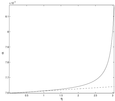
Figure 3.1: The evolution of $\alpha(\eta)$ and $a(\eta)$ for radiation-dominated universes with $\kappa=0$ (dashed) and $\kappa=1$ (solid).

As expected, we can see there is no difference in the evolution of $\alpha$ at early times and $\alpha\propto\eta$ as it was found in [1]. When the difference between the scale factors of the two universes becomes significant, the behaviour of $\alpha_{\kappa=1}$ begins to deviate from that of $\alpha_{\kappa=0}$. We see that $\alpha_{\kappa=1}$ clearly grows faster than $\alpha_{\kappa=0}$. The difference in the growth rates become very significant near the expansion maximum of the bound region ($\eta\approx\pi$). However, after this time our assumption that the background is not affected by changes of $\psi$ in the cosmological equations that describe the background universe breaks down, since the kinetic energy of the scalar field will diverge and can no longer be neglected in the Friedmann equation. We expect the behaviour near the final singularity to be similar to the kinetic-dominated evolution near the initial singularity discussed in ref. [108].

From figure 3.2 we see that the variations of $\alpha$ will become increasingly important as $\eta$ approaches the second singularity.

Figure 3.2: The evolution of $\frac{\delta\alpha}{\alpha}/\frac{\delta\rho_{r}}{\rho_{r}}$ vs $\eta$ in radiation-dominated universes.

Notice that although there is a considerable growth in the perturbations in $\alpha$, when we compare them with the perturbations in the radiation, they are not as significant as can be observed from the evolution of the ratio $\frac{\delta\alpha}{\alpha}/\frac{\delta\rho_{r}}{\rho_{r}}$ versus $\eta$ in figure 3.2.

3.5.2 Dust-dominated era

During the dust-dominated phase of a closed universe ($\kappa=1$) the normalised scale factor is given by $a=2\left(1-\cos(\eta)\right)$, while for a flat universe ($\kappa=0$) the normalised scale factor is given by $a=\ \eta^{2}$. Integrating equation (3.3.1) for both cases we obtain the evolution of $\alpha$ for both cases.

The evolution of $\alpha(\eta)$ can be seen in figure 3.3 along with the evolution of $a(\eta)$ for $\kappa=1,0$.

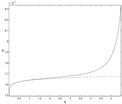
Figure 3.3: The evolution of $\alpha(\eta)$ and $a(\eta)$ for dust-dominated universes with $\kappa=0$ (dashed) and $\kappa=1$ (solid).

As in the radiation case, we can see there is little difference in the evolution of $\alpha$ at early times, since the scale factor for the closed model evolves very similarly to the flat one for $\eta<<1$ and $\alpha\propto\ln(\eta)$. The differences between $\alpha_{\kappa=1}$ and $\alpha_{\kappa=0}$ cases start to appear when $\eta\approx 1$, when the nonlinear regime commences. These differences become more accentuated near the second singularity, but once again this is the region where our approximations break down.

Notice that although there is a considerable growth in the perturbations in $\alpha$, when we compare them with the perturbations in the cold dark matter, they are not as significant as can be observed from the evolution of $\log(\frac{\delta\alpha}{\alpha})$ and $\log(\frac{\delta\rho_{m}}{\rho_{m}})$ $vs.$ $\log(\eta)$ in figure 3.4.

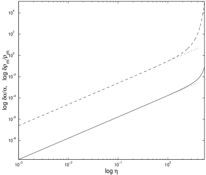
Figure 3.4: The evolution of $\log\frac{\delta\alpha}{\alpha}$ (solid) and $\log\frac{\delta\rho_{m}}{\rho_{m}}$ (dashed) vs $\log(\eta)$ for a dust-dominated universe. The dotted lines correspond to evolution in the linear perturbation solution.

In this case perturbations in $\alpha$ are even less significant than in the radiation case. We note that the fact that the linear regime is a very good approximation at early times, since as can be seen from figure 3.4, $\frac{\delta\alpha}{\alpha}$ tracks $\frac{\delta\rho_{m}}{\rho_{m}}\propto t^{2/3}$ at early times. From the detail of figure 3.4 we see that variations of the cold dark matter will start to occur before than variations of $\alpha$, and $\frac{\delta\rho_{m}}{\rho_{m}}$ is at least three orders of magnitude bigger than $\frac{\delta\alpha}{\alpha}$. This is an indication that perturbations in the matter fields will drive perturbations in $\alpha$.

3.6 Summary and Comments

The results presented in this chapter, are a quite good approximations when we consider large scales, but are expected to break down when extended to small scales, where non-linear effects come into play and local deviations from isotropy and homogeneity of the matter content are significant. We note that the background solutions for $\psi$, about which we have linearised the perturbations of the Einstein equations, are solutions which describe the time evolution of $\psi$ on a ’standard’ FRW background. Our neglect of the back-reaction of the $\psi$ perturbations on the background expansion dynamics is a good approximation up to logarithmic corrections.

When we examined the non-linear evolution of spherical inhomogeneities by means of a comparative numerical study of flat and closed Friedmann models we found that perturbations in $\alpha$ remain almost negligible with respect to perturbations in the fluid that dominates the energy density of the universe at the same epoch. Comparing the flat with the closed solution for $\alpha$, we concluded that in both the cases of a radiation or dust-dominated epoch, $\alpha$ will ’feel’ the change of behaviour in the scale factor, and the perturbations $\frac{\delta\alpha}{\alpha}$ will grow in time. The early-time behaviour of the non-linear solutions confirms the linear behaviour found previously. In particular $\frac{\delta\alpha}{\alpha}$ changes in proportion to $\frac{\delta\rho}{\rho}$ at early times.

We have provided a detailed analysis of the behaviour of inhomogeneous perturbations in $\alpha$ and its time variation on large scales under the assumption that the defining constant of the BSBM theory, $\zeta$, is constant and negative in sign. In reality this assumption will break down on small scales. The negativity of the effective value of $\zeta$ requires that the cold dark matter is dominated by the magnetic rather than the electric field energy (see also the discussion of reference [107] and by Bekenstein [83]). However, on sufficiently small scales the dark matter will become dominated by baryons and the sign of the effective $\zeta$ will have to change sign. Overall, there will also be a gradient in the value of $\left|\zeta\right|$ reflecting the scale dependence of the relative contribution of dark matter to the total density of the universe. We have not included these effects in the present analysis. They would need  to be included in any detailed analysis of the small-scale behaviour of inhomogeneities in $\alpha.$ This is an important challenge for future work because it would enable the quasar data on varying $\alpha$ to be compared directly with the limits from the Oklo natural reactor [8, 22] and Rhenium-Osmium abundances in meteorites [25, 21]. At present the relation between the cosmological and geonuclear evidences is unclear because the latter are derived from physical processes occurring within the cosmologically non-evolving solar system environment.

Variations of $\alpha$ also affect the cosmic microwave background radiation spectrum and anisotropy in different ways, but the effects must be disentangled from allowed changes in other cosmological parameters that can contribute similar effects. These changes in the microwave background with $\alpha$ left as a free constant parameter were analysed in [46] using the new WMAP data. They are far less sensitive that the many-multiplet analyses of quasars at $z=0.5-3.5$ [35, 5, 31, 32], although they derive from higher redshifts, $z<1100$. These studies can accommodate constant and varying $\alpha$ but up to a level that would be too large to be consistent with the quasar data and the slow time-evolution of the theory with time-varying $\alpha$ described in this thesis.

Chapter 4 Spherical Collapse Model in the Presence of Varying Alpha

…é neste horizonte do instante que se espelha a liberdade,
um rosto sem fundo sob um silêncio mudo: o éco da temporalidade.
– Ernesto Mota –

4.1 Introduction

In the last chapter, using the linear theory of the cosmological perturbations, it was shown that small inhomogeneities in the matter fields will induce small perturbations in the fine structure constant. Those results just confirmed our initial intuition that one cannot neglect the effects of gravity in the cosmological evolution of the fine structure constant. The reason is simple: any varying-$\alpha$ theory implies the existence of a field responsible for variations of the fine structure constant. This field is necessarily coupled to the matter fields, at least, to the ones which interact electromagnetically. Variations of $\alpha$, allowed by the conservation of energy and momentum will then depend on the expansion of the universe and the evolution of the electromagnetically coupled matter. Any inhomogeneities of the later will then affect the evolution of $\alpha$. In particular, spatial variations of the matter fields will then produce spatial variations of the fine structure constant. In reality, we will see in this chapter that not only the spatial homogeneity of $\alpha$ is affected by the growth of inhomogeneities in matter, but also its time evolution will change according to it. This effect is model independent since it is just a product of the coupling between the field responsible for the variations of $\alpha$ and matter. The inclusion of electroweak or grand unification theories will create even more general couplings, since the field, responsible for the $\alpha$-variations, may also be couple to all or some of the other matter fields, besides the ones that interact electromagnetically. Due to this, additional consequences will then result [111, 61].

It is useful to recall once again the present observational and experimental constraints that a successful varying-$\alpha$ model has to satisfy. We saw in chapter 1, that these constraints can be divided into two main groups: local and astro-cosmological. The local constraints derive from experiments in our local bound gravitational system: the Oklo natural reactor $(z=0.14)$, where $\left|\frac{\Delta\alpha}{\alpha}\right|\leq 10^{-7}$ [8]; the intra solar-system decay rate ${}^{187}\mathrm{Re}~{}\rightarrow~{}^{187}\mathrm{Os}$, $(z=0.45)$, where $\left|\frac{\Delta\alpha}{\alpha}\right|\leq 10^{-7}$ [57]; and the stability of terrestrial atomic clocks $(z=0)$, where $\left|\frac{\dot{\alpha}}{\alpha}\right|<4.2\times 10^{-15}~{}\mathrm{yr}^{-1}$[15]. Other limits arise from weak equivalence experiments [42] but the limits they provide are more model dependent. The astro-cosmological constraints are: the quasar absorption spectra $z=0.5-3.5$, where $\left|\frac{\Delta\alpha}{\alpha}\right|\approx 10^{-6}$; the cosmic microwave background radiation $(z=10^{3})$, where $\left|\frac{\Delta\alpha}{\alpha}\right|<10^{-2}$ [46] and Big Bang nucleosynthesis $(z=10^{8}-10^{10})$, where $\left|\frac{\Delta\alpha}{\alpha}\right|\leq 2\times 10^{-2}$ [46].

There is a potential discrepancy between local and astro-cosmological constraints; in particular, between the constraint of $\Delta\alpha/\alpha\leq 10^{-7}$ at redshift $z=0.45$, coming from the $\beta$-decay in meteoritic samples [57], and the explicit variation in $\alpha$ of $\Delta\alpha/\alpha\approx 10^{-6}$ at $z=0.5$, coming from the low-redshift end of the quasar absorption spectra [5]. A successful theory of varying $\alpha$ needs to explain this difference. This is a challenge. Models which use a very light scalar field, to drive variations in $\alpha$, need an extreme fine tuning in order to satisfy the phenomenological constraints coming from geochemical data (Oklo, $\beta$-decay), the present equivalent principle tests, and the quasar absorption spectra, simultaneously [22].

We will see in this chapter, that just by looking at the evolution of $\alpha$ in a universe where non-linear structures are formed, the discrepancy between geochemical constraints and the quasar data becomes “naturally” justified.

4.2 The Spherical Collapse Model

In order to study the behaviour of the fine structure constant during the formation of non-linear overdensities we will use the spherical infall model [128, 52, 157]. This will give us an idea on how the evolution of $\alpha$ in the overdensity “breaks away” from the corresponding one in the background.

An overdense sphere is a very useful non-linear model, as it behaves in exactly the same way as a closed sub-universe. The density perturbations need not to be a uniform sphere: any spherically symmetric perturbation will evolve at a given radius in the same way as a uniform sphere containing the same amount of mass [128]. In what follows, therefore, density refers to mean density inside a given sphere.

Let us consider a spherical perturbation with constant density inside it which, at an initial time, has an amplitude $\delta_{i}>0$ and $|\delta_{i}|\ll 1$. For the case of a flat matter-dominated FRW universe it is possible to find an exact solution for the evolution of the overdensity, although that is not the case for more complex cases, like ours, and a numerical simulation is required. Nevertheless the general behaviour of the overdensity will be similar. At early times the sphere expands together with the background. For a sufficiently large $\delta_{i}$ gravity prevents the sphere to expand forever. In that case, there are three interesting epochs in the final stages of its development. Turnaround: The sphere breaks away from the general expansion and reaches a maximum radius. Collapse: If only gravity operates, then the sphere will collapse to a singularity where the densities of the matter fields would go to infinity. In practise the collapse will never happen. As overdensities break away from the background expansion, Virialisation occurs, and they become gravitationally bounded systems through a process of violent relaxation [158, 159]. The underlying mechanism of violent relaxation is the chaotic gravitational field of a collapsing, non-spherical self-gravitational system. The time and space varying gravitational field provides the means for individual, non-interacting particles to change their energies and to become well mixed in phase space. After only a few dynamical times, ($\tau\sim(G\rho)^{-1/2}$) the result is a virialised distribution of matter whose phase space distribution is roughly Maxwellian and whose density varies as $\sim r^{-2}$ [128]. Due to its spherical symmetry and isothermal solution, such a configuration is referred as an isothermal sphere. In addition, baryonic matter can, through dissipative processes, lose energy and condense even further into cores of the isothermal spheres that form. The process of structure formation is much more complex and we shall not attempt to describe it here, referring the reader to [52, 128].

With virialisation, a condition of equilibrium is then reached and the system becomes stationary: There are no more variations of the radius of the system, or in its energy components. The stationary condition reached by the process of virialisation is very important, and affects dramatically the variations of the fine structure constant, as we will see bellow.

Once again we will use the BSBM theory in order to study the effects of structure formation in the evolution of $\alpha$. We will assume a $\Lambda$-Cold-Dark-Matter ($\Lambda CDM$) model of structure formation.

The background evolution of the universe and its components is given by the equations (1.7.7), (1.7.8) and equation (1.7). This equations will describe the evolution of the background scale factor, $a$, the scalar field, $\psi$, responsible for the variations of $\alpha$ and the energy density of non-relativistic matter $\rho_{m}$, respectively.

Just to clarify to notation from now on, we will label some variables which “live in” the background with a $b$. Quantities which “live” inside the overdensities will be labelled by $c$. For instance, the value of $\alpha$ inside a cluster will be referred to $\alpha_{c}$. Quantities which represent the epoch at or after virialisation, will be labelled by a $v$. For instance, $\Delta\alpha_{v}/\alpha_{v}$, represents the “time density contrast” at virialisation. This quantity represents a comparison between the value of the fine structure constant in a virialised clusters or in the background, at a given redshift, and its value on Earth, $\alpha_{0}$.

4.2.1 Dynamics of the overdensities

Variations of $\alpha$ inside overdense spherical regions can be studied using the spherical infall model. The evolution of a spherical overdense patch of scale radius $R(t)$ is given by the Friedmann acceleration equation:

$$\frac{\ddot{R}}{R}=-\frac{4\pi G}{3}\left(\rho_{cdm}\left(1+\left|\zeta\right|e^{-2\psi_{c}}\right)+4\rho_{\psi_{c}}-2\rho_{\Lambda}\right)$$ (4.2.1)

where $\rho_{cdm}$ is the total density of cold dark matter and baryons in the cluster, $\psi_{c}$ is the homogeneous field inside the cluster, $\rho_{\Lambda}$ is the cosmological constant density and $\rho_{\psi_{c}}\equiv\dot{\psi}_{c}^{2}/2$. We have used the equations of state $p_{\psi_{c}}=\rho_{\psi_{c}}$, $p_{cdm}=0$ and $p_{\Lambda}=-\rho_{\Lambda}$, where $p$ represents the pressure of the fluid.

In the cluster, the evolution of $\psi_{c}$ and $\rho_{cdm}$ are given by

$$\ddot{\psi_{c}}+3\frac{\dot{R}}{R}\dot{\psi_{c}} = -\frac{2}{\omega}e^{-2\psi_{c}}\zeta\rho_{cdm}$$ (4.2.2)

$$\dot{\rho}_{cdm} = -3\frac{\dot{R}}{R}\rho_{cdm}$$ (4.2.3)

According to the Virial theorem, a condition of equilibrium will be reached when

$$T=\frac{1}{2}R\frac{\partial U}{\partial R}$$ (4.2.4)

where, $T$ is the average total kinetic energy and $U$ is the average total potential energy in the sphere. Note that we obtain the usual $T=\frac{n}{2}U$ condition, for any potential with a powerlaw form ($U\propto R^{n}$), which will be our case.

The potential energy for a given component $x$ can be calculated from its general expression in a spherical region [160]:

$$U_{x} = 2\pi\int_{0}^{R}\rho_{tot}\phi_{x}r^{2}dr$$ (4.2.5)

$$\phi_{x}\left(r\right) = -2\pi G\rho_{x}\left(R^{2}-\frac{r^{2}}{3}\right)$$ (4.2.6)

where $\rho_{tot}$ is the total energy density inside the sphere, $\phi_{x}$ is the gravitational field potential due to the $\rho_{x}$ density component.

In the case of a $\Lambda CDM$ model the potential energies inside the cluster would be:

$$U_{G} = -\frac{3}{5}GM^{2}R^{-1}$$ (4.2.7)

$$U_{\Lambda} = -\frac{4}{5}\pi G\rho_{\Lambda}MR^{2}$$ (4.2.8)

$$U_{\psi_{c}} = -\frac{3}{5}GMM_{\psi_{c}}R^{-4}$$ (4.2.9)

where $U_{G}$ is the potential energy associated with the uniform spherical overdensity, $U_{\Lambda}$ is the potential associated with $\Lambda,$ and $U_{\psi_{c}}$ is the potential associated with $\psi_{c}.$ $M=M_{cdm}+M_{\psi_{c}}$ is the cluster mass, with

$$M_{cdm} = \frac{4\pi}{3}\rho_{cdm}(1+|\zeta|e^{-2\psi_{c}})R^{3}$$ (4.2.10)

$$M_{\psi_{c}} = \frac{4\pi}{3}\rho_{\psi_{c}}R^{6}$$ (4.2.11)

The virial theorem would be satisfied when:

$$T_{vir}=-\frac{1}{2}U_{G}+U_{\Lambda}-2U_{\psi_{c}}$$ (4.2.12)

where $T_{vir}$ $=\frac{1}{2}M\bar{v}_{vir}^{2}$ is the total kinetic energy at virialisation and $\bar{v}_{vir}^{2}$ is the mean-square velocity of masses in the cluster.

Using the virial theorem (4.2.12) and energy conservation at the turn around and when the cluster virialises, we obtain an equilibrium condition in term of the potential energies

$$\frac{1}{2}U_{G}(z_{v})+2U_{\Lambda}(z_{v})-U_{\psi_{c}}(z_{v})=U_{G}(z_{ta})+U_{\Lambda}(z_{ta})+U_{\psi_{c}}(z_{ta})$$ (4.2.13)

where $z_{v}$ is the redshift of virialisation and $z_{ta}$ is the redshift at the turn-around of the over-density at its maximum radius, when $R=R_{max}$ and $\dot{R}\equiv 0$. In the case where $\zeta=0$ and $\psi=\dot{\psi}=0$ we just have the usual virialisation condition for $\Lambda CDM$ models [161, 162].

The inclusion of a varying $\alpha$ at a level consistent with observation [35, 5, 30, 31, 32, 33], ($\dot{\alpha}/\alpha_{0}\sim 10^{-6}H$), does not affect the overall expansion of the universe up to logarithmic corrections, if we are far from the initial singularity [108]. The reason for that is the negligible contribution of $\psi$ to the energy content of the universe, see figure 1.2. In a similar way, the dynamical collapse of the overdense regions is also not affected: The energy density associated with $\psi_{c}$ is always a negligible contribution to the energy content of cluster. Even the kinetic energy, $\rho_{\psi_{c}}=\frac{\omega}{2}\dot{\psi}^{2}$, which starts to grow in the final stages of the cluster evolution will be negligible, see Figure 4.1.

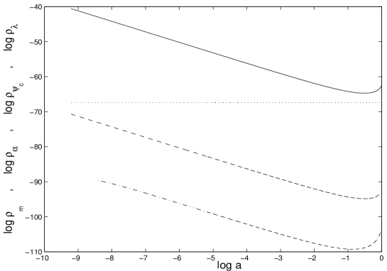
Figure 4.1: Evolution of $\log\rho_{cdm}$ (solid lines) , $\log\rho_{\psi_{c}}$ (dash-dotted line), $\log\rho_{\lambda}$ (dotted line) and $\log\rho_{\alpha}$ (dashed line) inside an overdensity, as a function of $\log(a)$, in a $\Lambda CDM$ model. Where $\rho_{\alpha}\equiv\rho_{\psi_{c}}+|\zeta|\rho_{cdm}e^{-2\psi_{c}}$.

4.3 Evolution of $\alpha$ During the Cluster Formation

The behaviour of the fine structure constant during the evolution of a cluster can now be obtained numerically evolving the background equations (1.7.7)-(1.7) and the cluster equations (4.2.1)-(4.2.3) until the virialisation condition holds, equation (4.2.13).

4.3.1 Setting the initial conditions

In order to satisfy the constraints imposed by the observations, we need to set up initial conditions for the evolution. Since the Earth is now a virialised overdense region, the initial condition for $\psi$ is chosen so as to obtain our measured laboratory value of $\alpha$ at virialisation, $\alpha_{c}(z_{v})\equiv\alpha_{v}=\alpha_{0}$. Since the redshift at which our cluster has virialised is uncertain, we will choose a representative example where virialisation occurs over the range $0<z_{v}<10$.

After we have set $z_{v}$ for Earth, another constraint we need to satisfy is given by the quasar observations [35]. This means that when comparing the value of the fine structure constant on Earth, at its virialisation, $\alpha_{v}=\alpha_{0}$, with the value of the fine structure constant of another region at some given redshift in the range accessed by the quasar spectra, $3.5\geq z\geq 0.5$, we need to obtain $\Delta\alpha/\alpha\equiv(\alpha(z)-\alpha_{v})/\alpha_{v}\approx-5.4\times 10^{-6}$. This raises the question as to the location of the clouds where the quasar absorption lines are formed: are they in a region which should be consider as part of the background or an overdensity with somewhat lower contrast than exists in our Galaxy? Unfortunately, this question cannot be answered because we do not know the density of the clouds, only the column density. Nevertheless, these clouds are much less dense than the solar system. Because of this, it is a good approximation to assume that the clouds possess the background density.

Thus, the initial conditions for $\psi$ are chosen so as to obtain our measured laboratory value of $\alpha$ at virialisation $\alpha_{c}(z_{v})=\alpha_{0}$ and to match the latest observations [35] for background regions at $3.5\geq|z-z_{v}|\geq 0.5$.

4.3.2 Differences between the background and the overdensities

Figure 4.2 show us the evolution of the fine structure constant inside an evolving overdensity and in the background. It is clear that there will be differences between the value of the fine structure constant inside a cluster, $\alpha_{c}$, and in the background, $\alpha_{b}$. It is also shown in that figure, that the value of $\alpha$ will also dependent on the redshift at which an overdensity will virialise.

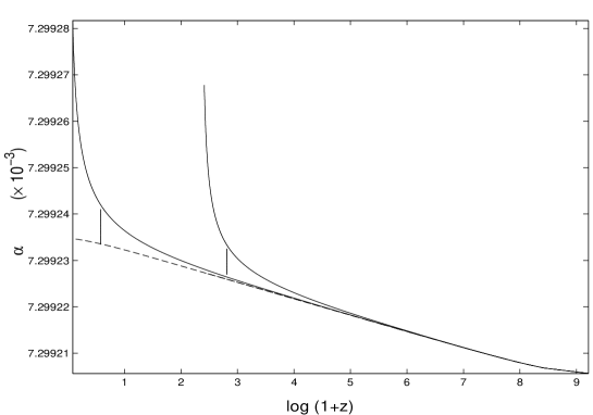
Figure 4.2: Evolution of $\alpha$ in the background (dashed line) and inside clusters (solid lines) as a function of $\log(1+z)$. Initial conditions were set to match observations of $\alpha$ variation of ref. [5]. Two clusters virialise at different redshifts, one of them in order to have ${}_{c}(z_{v}=1)=\alpha_{0}$. Vertical lines represent the moment of turn-around.

In figure 4.3, we have evolved four clusters, which have different initial conditions in order to satisfy the constraints described in the previous section.

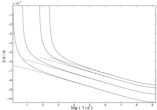
Figure 4.3: Evolution of $\Delta\alpha/\alpha$ in the background (dashed lines) and inside clusters (solid lines) as a function of $\log(1+z)$. Initial conditions were set to match observations of $\alpha$ variation of ref. [5]. Four clusters that virialised at different redshifts. All clusters were started so as to have $\alpha_{c}(z_{v})=\alpha_{0}$.

This is just an example, since in reality, the initial condition for $\psi$ needs to be fixed only once, for our Galaxy. Hence, $\alpha$ in other clusters will have a lower or higher value (with respect to $\alpha_{0}$) depending on their $z_{v}$; as can be seen in figure 4.2. The example given was just to show that independently of the redshift at which Earth virialises, the order of magnitude between virialised regions and the background is always of order $10^{-6}$. Of course this is not a coincidence, but a consequence of setting the initial conditions in order to satisfy the latest quasar observations [35]. This justifies why our study, although is a qualitative analysis, also can give us a good approximation of the order of magnitude expected for variations of the fine structure constant both inside overdensities and in the background. The choice of having assumed that the clouds, where the quasar observations were made, correspond to the background, is then a not very stringent condition.

4.3.3 Constancy of $\alpha$ after virialisation

After virialisation occurs, the cluster radius, $R$, becomes constant; time and space variations of $\alpha$ are suppressed, and $\alpha$ becomes constant. If there were any variations of $\alpha$ after virialisation, the energy components and radius of the cluster would need to vary in order to conserve energy and momentum. This would inconsistent with virialisation. This phenomenon is not included in figure 4.2, since we did follow the evolution to virialisation with a many-body simulation which would need to include the fluid equations that describe the pressure inside the cluster, see for instance [163, 164]. In our simulation, the virial condition is a ’stop condition’ and so we just observe the typical behaviour of the cluster’s collapse as $R\rightarrow 0$, see figure 4.4, or $\rho_{cdm}\rightarrow+\infty$, see figure 4.1.

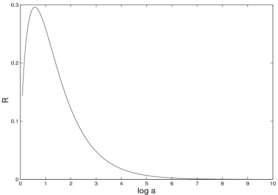
Figure 4.4: Evolution of the radius of a cluster, $R$, as a function of $\log(1+z)$.

In addition to the stationarity condition that occurs when the cluster virialises, it can be seen from figure 4.3 that in all cases the variation of $\alpha$ since the beginning of the cluster formation is of order $10^{-5}$, and numerical simulations give $\dot{\alpha}/\alpha\approx 10^{-22}s^{-1}$, we will see this in the next chapter. If variations of $\alpha$ are so small for such a wide range of virialisation redshifts, we can assume that the difference between the value of $\alpha_{c}$ at $z_{v}$ and at $z=0$ will be negligible. Therefore it is a good approximation to assume that the time-evolution of both $\alpha_{c}$ and of the cluster will cease after virialisation. Although this is not necessarily true ( for instance the cluster could keep accreting mass), it is a good approximation in respect of the evolution of $\alpha$, especially for clusters which have virialised at lower redshifts.

The fact that local $\alpha$ values ’freeze in’ at virialisation, means we would observe no time or spatial variations of $\alpha$ on Earth, or elsewhere in our Galaxy, even though time-variations in $\alpha$ might still be occurring on extragalactic scales. For a cluster, the value of $\alpha$ today will be the value of $\alpha$ at the virialisation time of the cluster. We should observe significant differences in $\alpha$ only when comparing clusters which virialised at quite different redshifts. Differences will arise within the same bound system only if it has not reached viral equilibrium. Hence, variations of $\alpha$ using geochemical methods could easily give a value that is $10-100$ times smaller than is inferred from quasar spectra. For instance, in spite of the fact that we cannot simulate the evolution of $\alpha_{c}$ after virialisation, it is useful to compare the value of $\Delta\alpha/\alpha$ in clusters that have have virialised at a low redshift and in the background, to have an order of magnitude of the variations in the fine structure constant. Numerical simulations, normalised to have $\alpha_{c}(z_{v}=0)=\alpha_{0}$ and to satisfy the quasar observations, give $\Delta\alpha/\alpha(z=2)=-6\times 10^{-6}$ for the background and $\Delta\alpha/\alpha(z_{v}=0.13)=-1.5\times 10^{-7}$ in a cluster which has virialised at $z_{v}=0.13$.

4.4 Measuring $\alpha$ in Virialised Regions

If we could measure the fine structure constant inside virialised overdensities and the corresponding value in the background, at the time of their virialisation, then figure 4.5 would give us the evolution of $\alpha_{v}$ or its time shift, $\Delta\alpha_{v}/\alpha_{v},$ as a function of $z_{v}$.

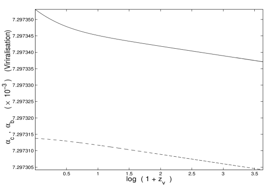
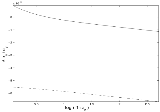
Figure 4.5: Plot of $\alpha$ and $\Delta\alpha/\alpha$ as a function of $\log(1+z)$, at virialisation. Clusters (solid line), background (dashed line).

Those figures show us that differences in $\alpha$ between the background and the overdensities increase as $z_{v}\rightarrow 0$. This is due to the earlier freezing of the value of $\alpha$ at virialisation, and to our assumption that we live in a $\Lambda CDM$ universe. At lower redshifts, specially after $\Lambda$ starts to dominate, variations of $\alpha$ in the background are turned off by the accelerated expansion. However, the value of $\alpha$ in the collapsing cluster will keep growing until virialisation occurs. At higher redshifts, $z\gg 1$, both $\alpha_{b}$ and $\alpha_{c}$ evolve in expanding environments: their increase is logarithmic in time before $\Lambda$ starts to dominate, so the difference between them will be much smaller.

These results mean that if we were able to compare the value of $\alpha$, in overdensities which have virialised at a similar redshift as ours, with regions that have virialised much before or much after, we would notice that there were indeed differences in the measured $\Delta\alpha/\alpha$.

4.4.1 Dependence on the matter density of the clusters

Variations of $\alpha_{c}$ with respect to $\alpha_{b}$ can be tracked using the “spatial density contrast”,

$$\frac{\delta\alpha}{\alpha}\equiv\frac{\alpha_{c}-\alpha_{b}}{\alpha_{b}},$$

and computed at virialisation or while the cluster is still evolving.

A plot of the “spatial density contrast” in $\alpha$ with respect to the matter density inhomogeneity, $\delta\rho/\rho,$ at virialisation is shown in figure. 4.6. Note that $\delta\alpha/\alpha$ grows in proportional to the density contrast of the matter inhomogeneities.

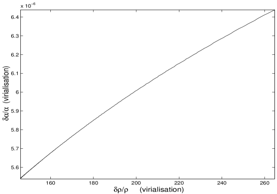
Figure 4.6: Variation of $\delta\alpha/\alpha$ with $\delta\rho/\rho$ at the cluster virialisation redshift. The evolution of $\alpha$ inside the clusters was normalised to satisfy the latest time-variation observational results, and to have $\alpha_{c}(z_{v})=\alpha_{0}$ for ${z}_{v}{=1.}$

In a $\Lambda CDM$ model, the density contrast, $\Delta_{c}=\rho_{cdm}(z_{v})/\rho_{b}(z_{v})$ increases as the redshift decreases [161]. For high redshifts, the density contrast at virialisation becomes the asymptotically constant in standard ($\Lambda=0$) $CDM$, $\Delta_{c}\approx 178$, if $\rho_{b}$ is measured at collapse or $\Delta_{c}\approx 148$, if $\rho_{b}$ is measured at virialisation. This is another reason why at lower redshifts the difference between $\alpha_{v}$ and $\alpha_{b}$ increases.

Trends of variation of $\alpha$ can be then predicted from the value of the matter density contrast of the regions observed. Useful fitting formulae for the dependence of $\alpha$ variation on $\delta\rho/\rho$ and the scale factor $a$ $\equiv(1+z)^{-1}$ are:

$$\frac{\delta\alpha}{\alpha} = (5.56-0.7\sigma^{\frac{1}{2}}+0.078\sigma+0.00352\sigma^{\frac{3}{2}})\times 10^{-6}$$

$$\frac{\delta\alpha}{\alpha} = (5.37+0.373\theta^{\frac{1}{6}}-0.27\theta^{\frac{1}{3}}+0.007\theta^{\frac{1}{2}})\times 10^{-6}$$ (4.4.1)

$$\frac{\Delta\alpha}{\alpha} = -(2.47-1.81\sigma^{\frac{1}{2}}+0.59\sigma-0.094\sigma^{\frac{3}{2}})\times 10^{-6}$$

where $\theta\equiv\frac{\delta\rho}{\rho}/\Delta_{c_{v}}$, $\sigma\equiv a/a_{v}$. $\Delta_{c_{v}}$ and $a_{v}$ are “input” parameters defined by our choice of the redshift of when $\alpha(z_{v})=\alpha_{0}$ . These formulae are valid for clusters which virialised at $0<z_{v}<15$. For the case where $\alpha(z_{v}=1)=\alpha_{0}$ these formulae are accurate to better than $1\%$.

4.5 Comments and Discussion

Generally, past studies of spatially homogeneous cosmologies have matched the value of $\alpha_{b}$ with the terrestrial value of $\alpha$ measured today. However, it is clear that the value of the fine structure constant on Earth, and most probably in our local cluster, will differ from that in the background universe. This feature has been ignored when comparing observations of $\alpha$ variations from quasar absorption spectra [35, 5, 31] with local bounds derived by direct measurement [165, 166] or from Oklo [20, 8, 22] and long-lived $\beta$-decayers [57]. A similar unwarranted assumption is generally made when using solar system tests of general relativity to bound possible time variations of $G$ in Brans-Dicke theory [167]: there is no reason why $\dot{G}/G$ should be the same in the solar system and on cosmological scales. Since any varying-constant model require the existence of a scalar field coupled to the matter fields, our considerations apply to all other theories besides BSBM and to variations of other “constants” [106, 7]. The consideration of the inhomogeneous evolution of the universe is therefore essential for a correct comparison of extra-galactic and solar system limits on, and observations of, possible time variation of the fine structure constant and other “constants”.

There are many different constraints, a theoretical model of varying-$\alpha$, needs to satisfy, in order to be in agreement with the observations and experiments. In particular, it needs to satisfy the geochemical constraints at, $z=0.45$, of $\Delta\alpha/\alpha<10^{-7}$ and the quasar data, at $z=0.5$, of $\Delta\alpha/\alpha\sim 10^{-6}$.

In order to explain, why any experiment made on earth [20, 8], or in our local system [167, 21], present constraints on variations of $\alpha$ which are, $10$ to $100$ times lower than the quasar spectra observations [35], we need to take into account the mechanism of structure formation in the universe. We have then considered that today’s value of $\alpha$ is measured on earth (and on our solar system), and that these are virialised overdensities. We have matched the quasar absorption spectra observations [35], comparing the today’s value of $\alpha$ on a virialised region (our galaxy) and the background (which represented the clouds where the quasar data was obtained). Using these assumption, to set up our initial conditions, we have used the spherical collapse model to investigate the effects of non-linear structure formation on the cosmological evolution of the fine structure constant. Evolving a tiny overdensity from the radiation era up to today, we were able to observe the differences between the evolution of $\alpha$ inside the overdensity and the background. When the density of these structures becomes big enough for them to break away from the background expansion, they start to collapse until its virialisation. When the overdensity virialises, variations of $\alpha$ are highly suppressed, and it becomes constant inside that region, otherwise the system would not be able to virialise.

The ’freeze in’ effect of the fine structure constant after virialisation is of major importance. Any experiment or observation made, in order to study variations of $\alpha$, on Earth or in our local system , would measure no variation at all. Or if they do, those would be much smaller than the results obtained from the quasar absorption spectra. So, variations of $\alpha$, would naturally satisfy any experiments on the violation of the principle of equivalence [56, 57, 58], in our local overdensity, and any geochemical observation. At the same time we would be able to explain the quasars absorption spectra observations [35, 5, 30, 31].

The dependence of $\alpha$ on the matter-field perturbations is much less important when one is studying effects on the early universe, for example on the CMBR or Big Bang nucleosynthesis [46]. In the linear regime of the cosmological perturbations, small perturbations in $\alpha$ will decay or become constant in the radiation era [2]. Also, in the non-linear regime of structure formation, the evolution of the fine structure constant in the background and inside the overdensities will not differ until the overdensities turnaround. Turnaround occurs at a far lower redshift than that of last scattering, $z=1100$. At these high redshifts, it was found that $\Delta\alpha/\alpha\leq 10^{-5}$. In the background, the fine structure constant, will be a constant during the radiation epoch [107]. A growth in value of $\alpha$ will happen only in the matter dominated era [1]. Hence, the early-universe constraint, coming from the CMBR and Big Bang Nucleosynthesis, $\Delta\alpha/\alpha\leq 10^{-2}$, are easily satisfied.

Chapter 5 The Fine Structure Constant Dependence on the Dark-Energy Equation of State and on the Coupling to Matter

O todo é tudo, e o mim que sou é o resto,
não há resto, há uma angustia isso sim
de saber que o todo que sou não o sei dizer…
mas o sei que sou todo assim…
– Ernesto Mota –

5.1 Introduction

In the last chapter, we saw that the cosmological evolution of the fine structure constant depends on the evolution of non-linear structures in the universe. There are two main features which affect the evolution of $\alpha$ in a universe where large scale structures are formed. The most obvious, is the coupling between the scalar field, which drives variations in $\alpha$, and the matter fields. The second is the dependence of non-linear models of structure formation on the equation of state of the universe, and in particular that of the dark energy one [161, 162].

Looking at the right-hand-side of equation (1.7.8), we see that, $\zeta/\omega$ represents the coupling between the scalar field $\psi$ an the matter density. It is then natural to think that the rate of change of the fine structure constant, both in the background and inside overdensities, will be a function of the absolute value of $\zeta/\omega$. Smaller values of $|\zeta/\omega|$ would lead to a smaller dependence of the variation of $\alpha$ on the matter inhomogeneities.

Besides the dependence on the coupling $\zeta/\omega$, the fine structure constant also depends on the equation of state of the universe. For instance, several solutions were found for $\alpha_{b}$, for the different epochs the universe went through. In the case of the overdensities, the dependence of $\alpha_{c}$ on the equation of state of the universe is related to the dependence of the density contrast of the overdensities on the structure formation model.

In resume, the evolution of the fine structure constant in the background, and inside clusters then depends mainly on the dominant equation of state of the universe and the value and sign of the coupling constant $\frac{\zeta}{\omega}$. We will then investigate the inhomogeneous evolution of the fine structure constant after the development of non-linear cosmic structures, that is, after they have virialised. This allow us to predict variations of the fine structure constant among virialised systems and to investigate the dependence of $\alpha$ on the equation of state of the dark energy. In the last section, we show how spatial variations in $\alpha$ may occur due to possible spatial variations in the coupling of $\alpha$ to the matter fields.

5.2 BSBM model and Dark Energy Structure Formation Models

In order to study the dependence of the evolution of $\alpha$ on the equation of state of dark energy, we need to generalise the equations used in the previous chapter both for the background and in the overdensities.

The background universe will be described by a flat, homogeneous and isotropic Friedmann metric with expansion scale factor $a(t)$. The universe contains pressure-free matter, of density $\rho_{m}$ $\propto a^{-3}$ and a dark energy fluid with a constant equation of state, $w_{\phi}$, and an energy-density $\rho_{\phi}\propto a^{-3(1+w_{\phi})}$. In the case where dark energy is the cosmological constant $\Lambda$, then $\rho_{\phi}\equiv\rho_{\Lambda}\equiv$ $\Lambda/(8\pi G)$ and $w_{\phi}=-1$. Hence the Friedmann equation (1.7.7) becomes:

$$H^{2}=\frac{8\pi G}{3}\left(\rho_{m}\left(1+\left|\zeta\right|e^{-2\psi}\right)\ +\rho_{\psi}+\rho_{\phi}\right)$$ (5.2.1)

The evolution of a spherical overdense patch of scale radius $R(t)$ is the given by the Friedmann acceleration equation (4.2.1), which becomes:

$$\frac{\ddot{R}}{R}=-\frac{4\pi G}{3}\left(\rho_{cdm}\left(1+\left|\zeta\right|e^{-2\psi_{c}}\right)+4\rho_{\psi_{c}}+(1+3w_{\phi_{c}})\rho_{\phi_{c}}\right)$$ (5.2.2)

where $\rho_{cdm}$ is the density of cold dark matter in the cluster, $\rho_{\phi_{c}}$ is the energy density of the dark energy inside the cluster and $\rho_{\psi_{c}}\equiv\frac{\omega}{2}\dot{\psi}_{c}^{2}$, where $\psi_{c}$ represents the scalar field inside the overdensity. We have also used the equations of state $p_{\psi_{c}}=\rho_{\psi_{c}}$, $p_{cdm}=0$ and $p_{\phi_{c}}=w_{\phi_{c}}\rho_{\phi_{c}}$.

In the cluster, the evolution of $\psi_{c}$, $\rho_{cdm}$ and $\rho_{\phi_{c}}$ are given by

$$\ddot{\psi_{c}}+3\frac{\dot{R}}{R}\dot{\psi_{c}} = -\frac{2}{\omega}e^{-2\psi_{c}}\zeta\rho_{cdm}$$ (5.2.3)

$$\dot{\rho}_{cdm} = -3\frac{\dot{R}}{R}\rho_{cdm}$$ (5.2.4)

$$\dot{\rho}_{\phi_{c}} = -3\frac{\dot{R}}{R}\left(1+w_{\phi_{c}}\right)\rho_{\phi_{c}}$$ (5.2.5)

Once again we will evolve our overdensity from a redshift well inside the radiation era until its virialisation occurs. In order to know when the cluster becomes virialised we will use the Virial theorem, equation (4.2.4). Again it will be useful to write the condition for virialisation to occur, using the potential energies associated to the different components of the overdensity.

Since we are now considering a dark energy fluid with a general, but constant, equation of state $w_{\phi_{c}}$, we need to generalise the potential energy associated to the cosmological constant, $U_{\Lambda}$. The generalisation of equation (4.2.9), in order to incorporate a fluid with a general equation of state is trivial. Using equations (4.2.6) and (4.2.9), we obtain the potential energy associated to the dark energy fluid

$$U_{\phi_{c}} = -\frac{3}{5}GM_{\phi_{c}}MR^{2-3\left(1+w_{\phi_{c}}\right)}$$ (5.2.6)

where $M_{\phi_{c}}$ is the mass associated to that fluid, given by

$$M_{\phi_{c}}=\frac{4\pi}{3}\rho_{\phi_{c}}R^{3\left(1+w_{\phi_{c}}\right)}.$$

Using now $U_{\phi_{c}}$ in equation (4.2.4), instead of $U_{\Lambda}$ we obtain a condition for virialisation, similar to equation (4.2.13), in terms of the known variables.

The behaviour of the fine structure constant during the evolution of a cluster can now be obtained numerically evolving the background equations (1.7.8) and (5.2.1) and the cluster equations (5.2.2)-(5.2.5) until the virialisation holds.

Once again the initial conditions for $\psi$ are chosen so as to obtain our measured laboratory value of $\alpha$ at virialisation $\alpha_{c}(z_{v})\equiv\alpha_{v}=\alpha_{0}$ and to match the latest observations [35]: $\Delta\alpha/\alpha\approx-5.4\times 10^{-6}$ for regions at $3.5\geq|z-z_{v}|\geq 0.5$, where $z_{v}$ will be the redshift at which our inhomogeneity virialised.

5.3 Dependence on the Dark-Energy Equation of Sate

Non-linear models of structure formation will present different features depending on the equation of state of the universe [161, 162]. The main difference is the way the parameter $\Delta_{c}=\rho_{cdm}(z_{c})/\rho_{b}(z_{v})$ evolves with the redshift. The evolution of $\Delta_{c}$ depends on the equation of state of the dark-energy component which dominates the expansion dynamics. For instance, in a $\Lambda CDM$ model, the density contrast, $\Delta_{c}$ increases as the redshift decreases. At high redshifts, the density contrast at virialisation becomes asymptotically constant in standard ($\Lambda=0$) $CDM$, with $\Delta_{c}\approx 178$ at collapse or $\Delta_{c}\approx 148$ at virialisation. This behaviour is common to other dark-energy models of structure formation ($wCDM$), where the major difference is in the magnitude and the rate of change of $\Delta_{c}$ at low redshifts.

The local value of the fine structure constant will be a function of the redshift and will be dependent on the density of the region of the universe we measure it, according to whether it is in the background or an overdensity [3]. The density contrast of the virialised clusters depends on the dark-energy equation of state parameter, $w_{\phi}$ . Hence, the evolution of $\alpha$ will be dependent on $w_{\phi}$ as well.

What difference we would expect to see in $\alpha$ if we compared two bound systems, like two clusters of galaxies? And how does the difference depend on the cosmological model of structure formation? These questions can be answered by looking at the time and spatial variations of $\alpha$ at the time of virialisation. The space variations will be tracked using a “spatial” density contrast,

$$\frac{\delta\alpha}{\alpha}\equiv\frac{\alpha_{c}-\alpha_{b}}{\alpha_{b}}$$ (5.3.1)

which is computed at virialisation (where $\alpha_{c}(z=z_{v})=\alpha_{v}$).

Since the main dependence of $\alpha$ is on the density of the clusters and the redshift of virialisation, we will only study dark-energy models where $w_{\phi}$ is a constant. Any effect contributed by a time-varying equation of state should be negligible, since the important feature is the average equation of state of the universe. This may not be the case for the models where the scalar field responsible for the variations in $\alpha$ is coupled to dark energy [168, 169, 170].

In order to have a qualitative behaviour of the evolution of the fine structure constant, at the virialisation of an overdensity, we will then compare the standard Cold Dark Matter model, $SCDM$, to the dark-energy Cold Dark Matter, $wCDM$, models. In particular, we will examine the representative cases of $w_{\phi}=-1,-0.8,-0.6$. All models will be normalised to have $\alpha_{v}=\alpha_{0}$ at $z=0$ and to satisfy the quasar observations [35], as discussed above. This normalisation, although unrealistic (Earth did not virialise today), give us some indication of the dependence of the time and spatial evolution in $\alpha$ on the different models. In reality, this approximation will not affect the order of magnitude of the spatial and time variations in $\alpha$ for the cases of virialisation at low redshift [3].

5.3.1 Time-shifts and the evolution of $\alpha$

The final value of $\alpha$ inside virialised overdensities and its evolution in the background is shown in figure 5.1. From this plot, a feature common to all the models stands out: the fine structure constant in the background regions has a lower value than inside the virialised overdensities. Also, its eventual local value depends on the redshift at which the overdensity virialises.

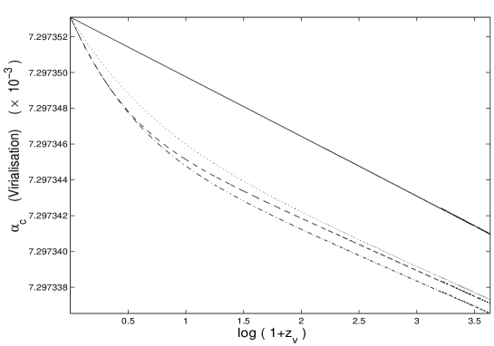
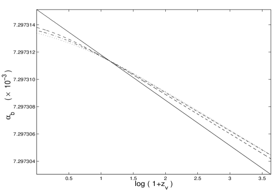
Figure 5.1: Value of $\alpha$ in the background and inside clusters as a function of $\log(1+z_{v})$, the epoch of virialisation. Solid line corresponds to the standard ($\Lambda=0$) $CDM$, dashed line is the $\Lambda CDM$, dashed-dotted corresponds to a $wCDM$ model with $w_{\phi}=-0.8$, dotted-line corresponds to a $wCDM$ model with $w_{\phi}=-0.6$. In all the models, the initial condition were set in order to have $\alpha_{c}(z=0)=\alpha_{0}$ and to satisfy $\Delta\alpha/\alpha\approx-5.4\times 10^{-6}$ at $3.5\geq|z-z_{v}|\geq 0.5$.

As expected, the equation of state of the dark energy affects the evolution of $\alpha,$ both in the overdensities and the background. A major difference arises if we compare the $SCDM$ and $wCDM$ models. In a $SCDM$ model, the fine structure constant is always a growing function, both in the background and inside the overdensities, and the growth rate is almost constant. In a $wCDM$ model, the evolution of $\alpha$ will depend strongly on whether one is inside a cluster or in the background. In the $wCDM$ background, $\alpha_{b}$ becomes constant (independent of the redshift) as the universe enters the phase of accelerated expansion. Inside the clusters, $\alpha_{v}$ will always grow and its value now will depend on the redshift at which virialisation occurred. The cumulative effect of this growth increases as we consider overdensities which virialise at increasingly lower redshift.

These differences arise due to the dependence of the fine structure constant on the equation of state of the universe and the density of the regions we are measuring it. In a $SCDM$ model, we will always live in a dust-dominated era. The fine structure constant will then be an ever-increasing logarithmic function of time, $\alpha\propto\ln(t)$ [107, 1]. The growth rates of $\alpha_{b}$ and $\alpha_{c}$ will be constant, since $\Delta_{c}$ is independent of the redshift in a $SCDM$ model. In a $wCDM$ model, dark energy plays an important role at low redshifts. As we reach low redshifts, where dark energy dominates the universal expansion, $\alpha_{b}$ becomes a constant [107, 1], but $\Delta_{c}$ continues to increase, as will $\alpha_{c}$ [3]. The growth of $\alpha_{v}$ becomes steeper as we go from a dark-energy fluid with $w_{\phi}=-0.6$ to the $\Lambda$-like case of $w_{\phi}=-1$. The intermediate situation is where $w_{\phi}=-0.8$, due to the dependence of $\Delta_{c}$ on $w_{\phi}$.

Similar conclusions can be drawn with respect to the “time shift” of the fine structure constant, ($\Delta\alpha/\alpha$), at virialisation, see figure 5.2

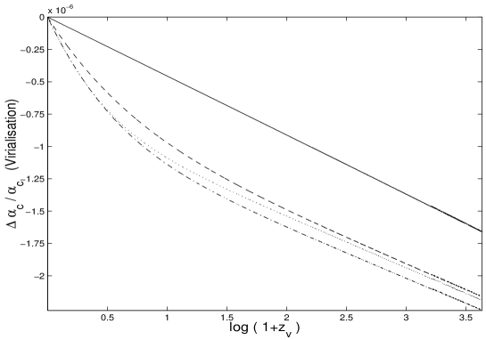
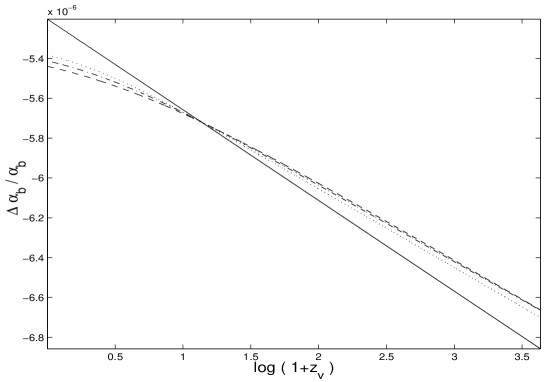
Figure 5.2: Variation of $\Delta\alpha/\alpha$ in the background and inside clusters as a function of the epoch of virialisation, $\log(1+z_{v})$. The solid line corresponds to the standard ($\Lambda=0$) $CDM$, the dashed line is the $\Lambda CDM$, the dashed-dotted line corresponds to a $wCDM$ model with $w_{\phi}=-0.8$, the dotted line corresponds to a $wCDM$ model with $w_{\phi}=-0.6$. In all models, the initial conditions were set in order to have $\alpha_{c}(z=0)=\alpha_{0}$ and to satisfy $\Delta\alpha/\alpha\approx-5.4\times 10^{-6}$ at $3.5\geq|z-z_{v}|\geq 0.5$.

5.3.2 Spatial variations in $\alpha$

Spatial variations in $\alpha$ will be dramatically different when comparing the standard $CDM$ model with the $wCDM$ models. In the $SCDM$ model, the difference between the fine structure constant in a virialised cluster ($\alpha_{v}$) and in the background ($\alpha_{b}$) will always be the same, $\delta\alpha/\alpha\approx 5.2\times 10^{-6}$, independently of the redshift at which we measure it, figure 5.3.

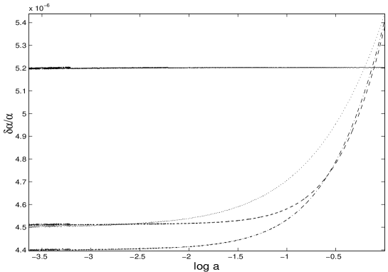
Figure 5.3: Variation of $\delta\alpha/\alpha$ as a function of $\log(1+z_{v})$. Solid line corresponds to the standard ($\Lambda=0$) $CDM$, dashed line is the $\Lambda CDM$, dashed-dotted line corresponds to a $wCDM$ model with $w_{\phi}=-0.8$, dotted line corresponds to a $wCDM$ model with $w_{\phi}=-0.6$. In all the models, the initial conditions were set in order to have $\alpha_{c}(z=0)=\alpha_{0}$ and to satisfy $\Delta\alpha/\alpha\approx-5.4\times 10^{-6}$ at $3.5\geq|z-z_{v}|\geq 0.5$.

Again, this is because, in a $SCDM$ model, $\Delta_{c}$ is always a constant independent of the redshift at which virialisation occurs. The constancy of $\delta\alpha/\alpha$ is a signature of the $SCDM$ structure-formation model, and it may even provide a means to rule out the $SCDM$ model completely if, when comparing the value of $\delta\alpha/\alpha$ in two different clusters, we do not find the same value, independently of $z_{v}$. A similar result is found for the case of a dark-energy structure formation model at high redshifts where $\delta\alpha/\alpha$ will be constant. This behaviour is expected since at high redshift any $wCDM$ model is asymptotically equivalent to standard $CDM$.

As expected, it is at low redshifts that the difference between $wCDM$ and $SCDM$ emerges. When comparing virialised regions at low redshifts, $\delta\alpha/\alpha$ will increase in a $wCDM$ model as we approach $z=0$. This is due to an increase of the density contrast of the virialised regions, $\Delta_{c}$, and the approach to a constant value of $\alpha_{b}$, see figure 5.4.

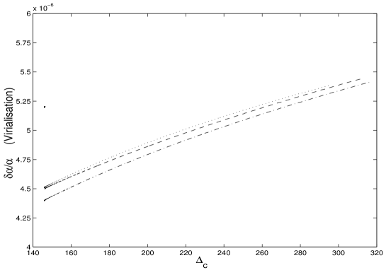
Figure 5.4: Variation of $\delta\alpha/\alpha$ as a function as a function of $\Delta_{c}$. The single-point corresponds to the standard ($\Lambda=0$) $CDM$, the dashed line is the $\Lambda CDM$, the dash-dot line corresponds to a $wCDM$ model with $w_{\phi}=-0.8$, dotted-line corresponds to a $wCDM$ model with $w_{\phi}=-0.6$. In all the models, the initial conditions were set in order to have $\alpha_{c}(z=0)=\alpha_{0}$ and to satisfy $\Delta\alpha/\alpha\approx-5.4\times 10^{-6}$ at $3.5\geq|z-z_{v}|\geq 0.5$.

In general, the growth will be steeper for smaller values of $w_{\phi}$, although there will be parameter degeneracies between the behaviour of different models, which ensure that there is no simple relation between $\delta\alpha/\alpha$ and the dark-energy equation of state. Note that, independently of the structure formation model we use, $\dot{\alpha}_{c}/\alpha_{c}$ at virialisation is always a decreasing function of time, as shown in figure 5.5.

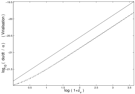
Figure 5.5: Variation of $log_{10}(\dot{\alpha}/\alpha)$ as a function of $log(1+z_{v})$. Solid line corresponds to the Standard ($\Lambda=0$) $CDM$, dashed-line is the $\Lambda CDM$, dashed-dotted corresponds to a $wCDM$ model with $w_{\phi}=-0.8$, dotted line corresponds to a $wCDM$ model with $w_{\phi}=-0.6$. In all the models, the initial conditions were set in order to have $\alpha_{c}(z=0)=\alpha_{0}$ and to satisfy $\Delta\alpha/\alpha\approx-5.4\times 10^{-6}$ at $3.5\geq|z-z_{v}|\geq 0.5$.

5.4 Dependence on the Coupling of $\alpha$ to the Matter Fields

The evolution of $\alpha$ in the background and inside clusters depends mainly on the dominant equation of state of the universe and the sign of the coupling constant $\zeta/\omega,$ which is determined by the theory and the dark matter’s identity. As was shown in chapter 2, $\alpha_{b}$ will be nearly constant for an accelerated expansion and also during the radiation era far from the initial singularity (where the kinetic term, $\rho_{\psi}$, can dominate).  Slow evolution of $\alpha$ will occur during the dust-dominated epoch, where $\alpha$ increases logarithmically in time for $\zeta<0$. When $\zeta$ is negative, $\alpha$ will be a slowly growing function of time but $\alpha$ will fall rapidly (even during a curvature-dominated era) for $\zeta$ positive [107]. A similar behaviour is found for the evolution of the fine structure constant inside overdensities. Thus, we see that a slow change in $\alpha$, cut off by the accelerated expansion at low redshift, that may be required by the data, demands that $\zeta<0$ in the cosmological background.

The sign of $\zeta$ is determined by the physical character of the matter that carries electromagnetic coupling. If it is dominated by magnetic energy then $\zeta<0$, if not then $\zeta>0.$ Baryons will usually have a positive $\zeta$ (although Bekenstein has argued for negative baryonic $\zeta$ in references [81, 82], but see [22]), in particular $\zeta\approx 10^{-4}$ for neutrons and protons. Dark matter may have negative values of $\zeta$, for instance superconducting cosmic strings have$\ \zeta\approx-1$.

In the previous section, we have chosen the sign of $\zeta$ to be negative so $\alpha$ is a slowly-growing function in time during the era of dust domination. This was done in order to match the latest observations which suggest that $\alpha$ had a smaller value in the past [5, 30, 31, 32]. This is a good approximation, since we have been studying the cosmological evolution of $\alpha$ during large-scale structure formation, when dark matter dominates. However, we know that on sufficiently small scales the dark matter will become dominated by a baryonic contribution for which $\zeta>0.$ The transition in the dominant form of total density, from non-baryonic to baryonic as one goes from large to small scales requires a significant evolution in the magnitude and sign of $\zeta/\omega$. This inhomogeneity will create distinctive behaviours in the evolution of the fine structure constant and will not be studied in this thesis. It is clear that a change in the sign of $\zeta/\omega$ will lead to a completely different type of evolution for $\alpha$, although the expected variations in the sign of $\zeta/\omega$ will occur on scales much smaller than those to which we are applying the spherical collapse model here. Hence, we will only investigate the effects of changing the absolute value of the coupling, $|\zeta/\omega|$, for the evolution of the fine structure constant.

From figure 5.6 it is clear that the rate of changes in $\alpha_{b}$ and $\alpha_{c}$ will be functions of the absolute value of $\zeta/\omega$. Smaller values of $|\zeta/\omega|$ lead to a slower variation of $\alpha$. A similar behaviour is found for the time variations in $\Delta\alpha/\alpha$, see figure 5.7.

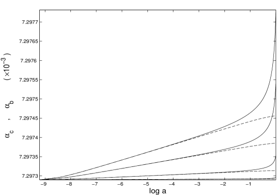
Figure 5.6: Evolution of $\alpha$ in the background (dashed-line) and inside a cluster (Solid line) as a function of $\log(1+z)$. For $\zeta/\omega=-10^{-4},-4\times 10^{-4},-7\times 10^{-4}$ and $-10^{-5}$. The lower curves correspond to a lower value of $\zeta/\omega$. The initial conditions were set in order to have $\alpha_{c}(z=0)=\alpha_{0}$ and to satisfy $\Delta\alpha/\alpha=-5.4\times 10^{-6}$ at $3\geq|z-z_{v}|\geq 1$, in the case where $\zeta=-7\times 10^{-4}$.

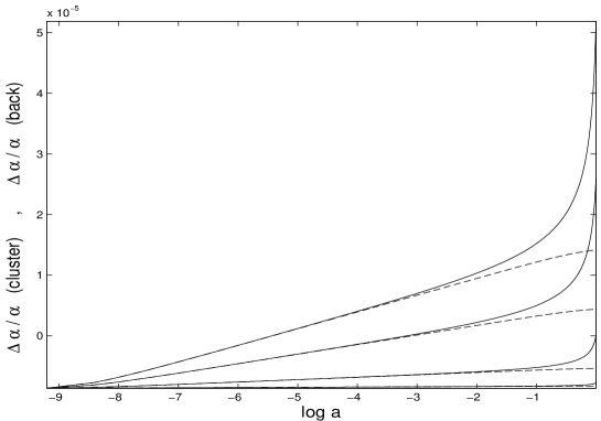
Figure 5.7: Evolution of $\Delta\alpha/\alpha$ in the background (dashed-line) and inside a cluster (Solid line) as a function of $\log(1+z)$. For $\zeta/\omega=-10^{-4},-4\times 10^{-4},-7\times 10^{-4}$ and $-10^{-5}$. The lower curves correspond to a lower value of $\zeta/\omega$. The initial conditions were set in order to have $\alpha_{c}(z=0)=\alpha_{0}$ and to satisfy $\Delta\alpha/\alpha=-5.4\times 10^{-6}$ at $3\geq|z-z_{v}|\geq 1$, in the case where $\zeta=-7\times 10^{-4}$.

The faster variation in $\alpha$ and $\Delta\alpha/\alpha$ for higher values of $|\zeta/\omega|$ is also a common feature for $\delta\alpha/\alpha$, see figure 5.8. This is expected. A stronger coupling to the matter fields would naturally lead to a stronger dependence on the matter inhomogeneities, and in particular on their density contrast, $\Delta_{c}$.

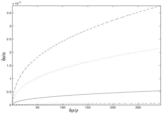
Figure 5.8: Evolution of $\delta\alpha/\alpha$ as a function $\delta\rho/\rho$. For $\zeta/\omega=-10^{-4},-4\times 10^{-4},-7\times 10^{-4}$ and $-10^{-5}$. The lower curves correspond to a lower value of $\zeta/\omega$. The initial conditions were set in order to have $\alpha_{c}(z=0)=\alpha_{0}$ and to satisfy $\Delta\alpha/\alpha\approx-5.4\times 10^{-6}$ at $3\geq|z-z_{v}|\geq 1$, in the case where $\zeta=-7\times 10^{-4}$.

In reality, the dependence of $\alpha$ on the coupling $\zeta/\omega$ has a degeneracy with respect to the initial condition chosen for $\psi$. This is clear from the scale invariance of equation (1.7.8) under linear shifts in the value of $\psi\rightarrow\psi+const$ and rescaling of $\zeta/\omega$ and $t$. It is always possible, to obtain the same evolution (and rate of change) of $\alpha$ and $\Delta\alpha/\alpha$ for any other value of $|\zeta/\omega|$; see for example Tables 5.1,5.2,5.3 and 5.4, where we have tabulated the shifts $\Delta\alpha/\alpha,\delta\alpha/\alpha,$ and time change, $\dot{\alpha}/\alpha,$ obtained in the clusters and in the background for various numerical choices of $\zeta/\omega$ and virialisation redshift $z_{v}$. The observed Oklo and $\beta$-decay constraints on variations in $\alpha$ are highlighted in italic and boldface, respectively.

$z_{v}$	$\frac{\Delta\alpha}{\alpha}|_{b}\times 10^{-6}$	$\frac{\Delta\alpha}{\alpha}|_{c}\times 10^{-7}$	$\frac{\dot{\alpha}}{\alpha}|_{b}\times 10^{-24}$	$\frac{\dot{\alpha}}{\alpha}|_{c}\times 10^{-22}$	$\frac{\delta\alpha}{\alpha}\times 10^{-6}$
$0.00$	$-5.381$	$0.000$	$0.361$	$1.068$	$5.38$
${\it{0.09}}$	${\it{-5.397}}$	${\it{-1.618}}$	${\it{0.427}}$	${\it{1.128}}$	${\it{5.24}}$
$0.18$	$-5.412$	$-2.889$	$0.493$	$1.192$	$5.12$
$0.26$	$-5.427$	$-3.915$	$0.558$	$1.260$	$5.04$
$0.34$	$-5.442$	$-4.769$	$0.623$	$1.329$	$4.97$
${\bf{0.41}}$	${\bf{-5.456}}$	${\bf{-5.485}}$	${\bf{0.688}}$	${\bf{1.401}}$	${\bf{4.91}}$
$0.49$	$-5.470$	$-6.097$	$0.753$	$1.475$	$4.86$
$0.51$	$-5.474$	$-6.271$	$0.773$	$1.498$	$4.85$
$0.61$	$-5.492$	$-6.941$	$0.860$	$1.601$	$4.80$
$0.70$	$-5.509$	$-7.510$	$0.948$	$1.708$	$4.76$
$0.80$	$-5.526$	$-8.001$	$1.036$	$1.816$	$4.73$
$0.89$	$-5.542$	$-8.427$	$1.124$	$1.928$	$4.70$
$0.95$	$-5.552$	$-8.684$	$1.184$	$2.005$	$4.68$
$1.07$	$-5.572$	$-9.139$	$1.303$	$2.161$	$4.66$
$1.19$	$-5.590$	$-9.534$	$1.424$	$2.321$	$4.64$
$1.30$	$-5.608$	$-9.882$	$1.546$	$2.484$	$4.62$
$1.36$	$-5.617$	$-10.048$	$1.608$	$2.569$	$4.61$
$1.51$	$-5.639$	$-10.428$	$1.773$	$2.793$	$4.60$
$1.66$	$-5.660$	$-10.767$	$1.940$	$3.024$	$4.58$
$1.76$	$-5.674$	$-10.973$	$2.053$	$3.181$	$4.58$
$1.95$	$-5.699$	$-11.333$	$2.278$	$3.496$	$4.57$
$2.14$	$-5.722$	$-11.658$	$2.508$	$3.821$	$4.56$
$2.15$	$-5.723$	$-11.670$	$2.519$	$3.838$	$4.56$
$2.40$	$-5.751$	$-12.035$	$2.824$	$4.272$	$4.55$
$2.54$	$-5.767$	$-12.237$	$3.009$	$4.535$	$4.54$
$2.85$	$-5.799$	$-12.624$	$3.417$	$5.121$	$4.54$
$2.92$	$-5.807$	$-12.711$	$3.521$	$5.272$	$4.54$
$3.31$	$-5.843$	$-13.129$	$4.055$	$6.043$	$4.53$
$3.69$	$-5.876$	$-13.495$	$4.612$	$6.852$	$4.53$
$4.07$	$-5.906$	$-13.835$	$5.190$	$7.690$	$4.52$
$4.45$	$-5.935$	$-14.137$	$5.788$	$8.562$	$4.52$
$4.83$	$-5.961$	$-14.415$	$6.407$	$9.466$	$4.52$

Table 5.1: $\frac{\zeta}{\omega}=-10^{-1}$: Time and space variations in $\alpha$ obtained for the corresponding redshifts of virialisation, $z_{v}$, for $\zeta/\omega=-10^{-1}$. We have assumed a $\Lambda CDM$ model. The indexes ${}^{\prime}b^{\prime}$ and ${}^{\prime}c^{\prime}$, stand for background and cluster respectively. The italic and bold entries correspond approximately to the level of the Oklo and $\beta$-decay rate constraints, respectively. The quasar absorption spectra observations correspond to the values of $\Delta\alpha/\alpha|_{b}$. The initial conditions were set in order to have $\alpha_{c}(z=0)=\alpha_{0}$.

$z_{v}$	$\frac{\Delta\alpha}{\alpha}|_{b}\times 10^{-6}$	$\frac{\Delta\alpha}{\alpha}|_{c}\times 10^{-7}$	$\frac{\dot{\alpha}}{\alpha}|_{b}\times 10^{-24}$	$\frac{\dot{\alpha}}{\alpha}|_{c}\times 10^{-22}$	$\frac{\delta\alpha}{\alpha}\times 10^{-6}$
$0.00$	$-5.382$	$0.000$	$0.361$	$1.068$	$5.38$
${\it{0.09}}$	${\it{-5.398}}$	${\it{-1.618}}$	${\it{0.427}}$	${\it{1.128}}$	${\it{5.24}}$
$0.18$	$-5.414$	$-2.889$	$0.493$	$1.193$	$5.12$
$0.26$	$-5.429$	$-3.916$	$0.558$	$1.260$	$5.04$
$0.34$	$-5.443$	$-4.769$	$0.623$	$1.329$	$4.97$
${\bf{0.41}}$	${\bf{-5.458}}$	${\bf{-5.486}}$	${\bf{0.688}}$	${\bf{1.401}}$	${\bf{4.91}}$
$0.49$	$-5.471$	$-6.098$	$0.753$	$1.475$	$4.86$
$0.51$	$-5.476$	$-6.272$	$0.773$	$1.498$	$4.85$
$0.61$	$-5.493$	$-6.943$	$0.860$	$1.602$	$4.80$
$0.70$	$-5.511$	$-7.511$	$0.948$	$1.708$	$4.76$
$0.80$	$-5.527$	$-8.003$	$1.036$	$1.817$	$4.73$
$0.89$	$-5.543$	$-8.428$	$1.124$	$1.929$	$4.70$
$0.95$	$-5.553$	$-8.685$	$1.184$	$2.006$	$4.68$
$1.07$	$-5.573$	$-9.141$	$1.303$	$2.161$	$4.66$
$1.19$	$-5.592$	$-9.535$	$1.424$	$2.321$	$4.64$
$1.30$	$-5.610$	$-9.884$	$1.546$	$2.485$	$4.62$
$1.36$	$-5.619$	$-10.050$	$1.609$	$2.569$	$4.61$
$1.51$	$-5.641$	$-10.430$	$1.773$	$2.794$	$4.60$
$1.66$	$-5.662$	$-10.769$	$1.940$	$3.025$	$4.58$
$1.76$	$-5.675$	$-10.976$	$2.053$	$3.182$	$4.58$
$1.95$	$-5.700$	$-11.336$	$2.278$	$3.497$	$4.57$
$2.14$	$-5.723$	$-11.660$	$2.508$	$3.822$	$4.56$
$2.15$	$-5.725$	$-11.672$	$2.520$	$3.839$	$4.56$
$2.40$	$-5.753$	$-12.038$	$2.825$	$4.273$	$4.55$
$2.54$	$-5.769$	$-12.239$	$3.009$	$4.536$	$4.54$
$2.85$	$-5.801$	$-12.626$	$3.417$	$5.122$	$4.54$
$2.92$	$-5.808$	$-12.713$	$3.522$	$5.273$	$4.54$
$3.31$	$-5.844$	$-13.132$	$4.056$	$6.045$	$4.53$
$3.69$	$-5.877$	$-13.498$	$4.613$	$6.853$	$4.53$
$4.07$	$-5.908$	$-13.837$	$5.191$	$7.692$	$4.52$
$4.45$	$-5.936$	$-14.140$	$5.790$	$8.565$	$4.52$
$4.83$	$-5.962$	$-14.418$	$6.408$	$9.469$	$4.52$

Table 5.2: $\frac{\zeta}{\omega}=-10^{-4}$: Time and space variations in $\alpha$ obtained for the corresponding redshifts of virialisation, $z_{v}$, for $\zeta/\omega=-10^{-4}$. We have assumed a $\Lambda CDM$ model. The indexes ${}^{\prime}b^{\prime}$ and ${}^{\prime}c^{\prime}$, stand for background and cluster respectively. The italic and bold entries correspond approximately to the level of the Oklo and $\beta$-decay rate constraints, respectively. The quasar absorption spectra observations correspond to the values of $\Delta\alpha/\alpha|_{b}$. The initial conditions were set in order to have $\alpha_{c}(z=0)=\alpha_{0}$.

$z_{v}$	$\frac{\Delta\alpha}{\alpha}|_{b}\times 10^{-6}$	$\frac{\Delta\alpha}{\alpha}|_{c}\times 10^{-7}$	$\frac{\dot{\alpha}}{\alpha}|_{b}\times 10^{-24}$	$\frac{\dot{\alpha}}{\alpha}|_{c}\times 10^{-22}$	$\frac{\delta\alpha}{\alpha}\times 10^{-6}$
$0.00$	$-5.381$	$0.000$	$0.361$	$1.068$	$5.38$
${\it{0.09}}$	${\it{-5.397}}$	${\it{-1.617}}$	${\it{0.427}}$	${\it{1.128}}$	${\it{5.24}}$
$0.18$	$-5.413$	$-2.889$	$0.493$	$1.192$	$5.12$
$0.26$	$-5.428$	$-3.915$	$0.558$	$1.260$	$5.04$
$0.34$	$-5.442$	$-4.768$	$0.623$	$1.329$	$4.97$
${\bf{0.41}}$	${\bf{-5.457}}$	${\bf{-5.485}}$	${\bf{0.688}}$	${\bf{1.401}}$	${\bf{4.91}}$
$0.49$	$-5.470$	$-6.097$	$0.753$	$1.475$	$4.86$
$0.51$	$-5.475$	$-6.271$	$0.773$	$1.498$	$4.85$
$0.61$	$-5.492$	$-6.941$	$0.860$	$1.601$	$4.80$
$0.70$	$-5.510$	$-7.510$	$0.948$	$1.708$	$4.76$
$0.80$	$-5.526$	$-8.001$	$1.036$	$1.817$	$4.73$
$0.89$	$-5.542$	$-8.427$	$1.124$	$1.929$	$4.70$
$0.95$	$-5.552$	$-8.684$	$1.184$	$2.006$	$4.68$
$1.07$	$-5.572$	$-9.139$	$1.303$	$2.161$	$4.66$
$1.19$	$-5.591$	$-9.534$	$1.424$	$2.321$	$4.64$
$1.30$	$-5.609$	$-9.882$	$1.546$	$2.485$	$4.62$
$1.36$	$-5.618$	$-10.048$	$1.608$	$2.569$	$4.61$
$1.51$	$-5.640$	$-10.428$	$1.773$	$2.794$	$4.60$
$1.66$	$-5.661$	$-10.767$	$1.940$	$3.024$	$4.58$
$1.76$	$-5.674$	$-10.973$	$2.053$	$3.181$	$4.58$
$1.95$	$-5.699$	$-11.334$	$2.278$	$3.497$	$4.57$
$2.14$	$-5.722$	$-11.658$	$2.508$	$3.822$	$4.56$
$2.15$	$-5.724$	$-11.670$	$2.519$	$3.838$	$4.56$
$2.40$	$-5.752$	$-12.036$	$2.824$	$4.272$	$4.55$
$2.54$	$-5.768$	$-12.237$	$3.009$	$4.535$	$4.54$
$2.85$	$-5.800$	$-12.624$	$3.417$	$5.121$	$4.54$
$2.92$	$-5.807$	$-12.711$	$3.521$	$5.272$	$4.54$
$3.31$	$-5.843$	$-13.129$	$4.056$	$6.044$	$4.53$
$3.69$	$-5.876$	$-13.495$	$4.612$	$6.852$	$4.53$
$4.07$	$-5.907$	$-13.835$	$5.190$	$7.690$	$4.52$
$4.45$	$-5.935$	$-14.137$	$5.789$	$8.563$	$4.52$
$4.83$	$-5.961$	$-14.415$	$6.407$	$9.467$	$4.52$

Table 5.3: $\frac{\zeta}{\omega}=-10^{-6}$: Time and space variations in $\alpha$ obtained for the corresponding redshifts of virialisation, $z_{v}$, for $\zeta/\omega=-10^{-6}$. We have assumed a $\Lambda CDM$ model. The indexes ${}^{\prime}b^{\prime}$ and ${}^{\prime}c^{\prime}$, stand for background and cluster respectively. The italic and bold entries correspond approximately to the level of the Oklo and $\beta$-decay rate constraints, respectively. The quasar absorption spectra observations correspond to the values of $\Delta\alpha/\alpha|_{b}$. The initial conditions were set in order to have $\alpha_{c}(z=0)=\alpha_{0}$.

$z_{v}$	$\frac{\Delta\alpha}{\alpha}|_{b}\times 10^{-6}$	$\frac{\Delta\alpha}{\alpha}|_{c}\times 10^{-7}$	$\frac{\dot{\alpha}}{\alpha}|_{b}\times 10^{-24}$	$\frac{\dot{\alpha}}{\alpha}|_{c}\times 10^{-22}$	$\frac{\delta\alpha}{\alpha}\times 10^{-6}$
$0.00$	$-5.385$	$0.000$	$0.361$	$1.068$	$5.38$
${\it{0.09}}$	${\it{-5.401}}$	${\it{-1.619}}$	${\it{0.428}}$	${\it{1.129}}$	${\it{5.24}}$
$0.18$	$-5.416$	$-2.891$	$0.493$	$1.193$	$5.13$
$0.26$	$-5.431$	$-3.918$	$0.559$	$1.261$	$5.04$
$0.34$	$-5.446$	$-4.772$	$0.624$	$1.330$	$4.97$
${\bf{0.41}}$	${\bf{-5.460}}$	${\bf{-5.489}}$	${\bf{0.689}}$	${\bf{1.402}}$	${\bf{4.91}}$
$0.49$	$-5.474$	$-6.101$	$0.753$	$1.476$	$4.86$
$0.51$	$-5.478$	$-6.275$	$0.773$	$1.499$	$4.85$
$0.61$	$-5.496$	$-6.946$	$0.861$	$1.602$	$4.80$
$0.70$	$-5.513$	$-7.515$	$0.948$	$1.709$	$4.76$
$0.80$	$-5.530$	$-8.007$	$1.036$	$1.818$	$4.73$
$0.89$	$-5.546$	$-8.432$	$1.125$	$1.930$	$4.70$
$0.95$	$-5.556$	$-8.690$	$1.185$	$2.007$	$4.69$
$1.07$	$-5.576$	$-9.145$	$1.304$	$2.162$	$4.66$
$1.19$	$-5.595$	$-9.540$	$1.425$	$2.322$	$4.64$
$1.30$	$-5.613$	$-9.889$	$1.547$	$2.486$	$4.62$
$1.36$	$-5.621$	$-10.055$	$1.610$	$2.571$	$4.62$
$1.51$	$-5.644$	$-10.435$	$1.774$	$2.795$	$4.60$
$1.66$	$-5.664$	$-10.774$	$1.941$	$3.026$	$4.59$
$1.76$	$-5.678$	$-10.981$	$2.054$	$3.183$	$4.58$
$1.95$	$-5.703$	$-11.341$	$2.279$	$3.499$	$4.57$
$2.14$	$-5.726$	$-11.666$	$2.510$	$3.824$	$4.56$
$2.15$	$-5.727$	$-11.678$	$2.521$	$3.841$	$4.56$
$2.40$	$-5.756$	$-12.044$	$2.826$	$4.275$	$4.55$
$2.54$	$-5.771$	$-12.245$	$3.011$	$4.538$	$4.55$
$2.85$	$-5.803$	$-12.633$	$3.419$	$5.125$	$4.54$
$2.92$	$-5.811$	$-12.719$	$3.523$	$5.276$	$4.54$
$3.31$	$-5.847$	$-13.138$	$4.058$	$6.048$	$4.53$
$3.69$	$-5.880$	$-13.505$	$4.615$	$6.857$	$4.53$
$4.07$	$-5.911$	$-13.844$	$5.193$	$7.695$	$4.53$
$4.45$	$-5.939$	$-14.147$	$5.792$	$8.569$	$4.52$
$4.83$	$-5.965$	$-14.425$	$6.412$	$9.473$	$4.52$

Table 5.4: $\frac{\zeta}{\omega}=-10^{-10}$: Time and space variations in $\alpha$ obtained for the corresponding redshifts of virialisation, $z_{v}$, for $\zeta/\omega=-10^{-10}$. We have assumed a $\Lambda CDM$ model. The indexes ${}^{\prime}b^{\prime}$ and ${}^{\prime}c^{\prime}$, stand for background and cluster respectively. The italic and bold entries correspond approximately to the level of the Oklo and $\beta$-decay rate constraints, respectively. The quasar absorption spectra observations correspond to the values of $\Delta\alpha/\alpha|_{b}$. The initial conditions were set in order to have $\alpha_{c}(z=0)=\alpha_{0}$.

In the plots of this section, we have chosen the value $\zeta/\omega=-7\times 10^{-4}$ to be the one which satisfies the current observations, but we could have used any value of $|\zeta/\omega|$ because of the invariance under rescalings. However, once we set the initial condition for a given value of $\zeta/\omega$, any deviation from that value leads to quite different future variations in $\alpha$. This can occur if there are regions of the universe where the dominant matter has a different nature, and do possesses a different value (and even sign) of $\zeta/\omega$ to that in our solar system. The evolution of $\alpha$ in those regions may then be different from the one that led to the value of $\alpha_{c}(z=z_{v})=\alpha_{0}$ on Earth.

It is important to note that, due to the degeneracy between the initial condition and the coupling to the matter fields, there is no way to avoid evolving differences in $\alpha$ variations between the overdensities and the background. The difference will be of the same order of magnitude as the effects indicated by the recent quasar absorption-line data. This is not a coincidence and it is related to the fact that we have normalised $\alpha(z=z_{v})=\alpha_{0}$ on Earth and $\Delta\alpha/\alpha=5.4\times 10^{-6}$ at $3.5\geq|z-z_{v}|\geq 0.5$. So, any varying-$\alpha$ model that uses these normalisations will create a similar difference in $\alpha$ evolution between the overdensities and the background, independently of the coupling $\zeta/\omega$.

We might ask: how model-independent are these results? In this connection it is interesting to note that even with a zero coupling to the matter fields (which is unrealistic), $\zeta=0$, there is no way to avoid difference arising between the evolution of $\alpha$ in the background and in the cluster overdensities. While the background expansion has a monotonically-increasing scale factor, $a(t)$, the overdensities will have a scale radius, $R(t)$, which will eventually collapse at a finite time. For instance, in the case where $\zeta=0$, equations (1.7.8) and (5.2.3) can be automatically integrated to give:

$$\dot{\psi} \propto a^{-3}$$ (5.4.1)

$$\dot{\psi}_{c} \propto R^{-3}$$ (5.4.2)

The difference between those two solutions clearly increases, especially after the turnaround of the overdensity, when that region starts to collapse. As the collapse proceeds, the bigger will be the difference between the background and the overdensity. Variations in $\alpha$ between the background and the overdensities are therefore quite natural although they have always been ignored in studies of varying constants in cosmology.

5.5 Discussion of the Results and Observational Constraints

The development of matter inhomogeneities in our universe affects the cosmological evolution of the fine structure constant [2, 3]. Therefore, variations in $\alpha$ depend on nature of its coupling to the matter fields and the detailed large-scale structure formation model. Large-scale structure formation models depend in turn on the dark-energy equation of state. This dependence is particularly strong at low redshifts, when dark energy dominates the density of the universe [161, 162]. Using the BSBM varying-$\alpha$ theory, and the simplest spherical collapse model, we have studied the effects of the dark-energy equation of state and the coupling to the matter fields on the evolution of the fine structure constant. We have compared the evolution of $\alpha$ inside virialised overdensities, using the standard ($\Lambda=0$) $CDM$ model of structure formation and dark-energy modification ($wCDM$). It was shown that, independently of the model of structure formation one considers, there is always a spatial contrast, $\delta\alpha/\alpha$, between $\alpha$ in an overdensity and in the background. In a $SCDM$ model, $\delta\alpha/\alpha$ is always a constant, independent of the virialisation redshift, see Table 5.5. In the case of a $wCDM$ model, especially at low redshifts, the spatial contrast depends on the time when virialisation occurs and the equation of state of the dark energy. At high redshifts, when the $wCDM$ model becomes asymptotically equivalent to the $SCDM$ one, $\delta\alpha/\alpha$ is a constant. At low redshifts, when dark energy starts to dominate, the difference between $\alpha$ in a cluster and in the background grows. The growth rate is proportional to $|w_{\phi}|$, see Tables 5.6, 5.7 and 5.8. These differences in the behaviour of the fine structure constant, its “time shift density contrast” ($\Delta\alpha/\alpha$) and its “spatial density contrast” ($\delta\alpha/\alpha$) could help us to distinguish among different dark-energy models of structure formation at low redshifts.

$z_{v}$	$\frac{\Delta\alpha}{\alpha}|_{b}\times 10^{-6}$	$\frac{\Delta\alpha}{\alpha}|_{c}\times 10^{-7}$	$\frac{\dot{\alpha}}{\alpha}|_{b}\times 10^{-24}$	$\frac{\dot{\alpha}}{\alpha}|_{c}\times 10^{-22}$	$\frac{\delta\alpha}{\alpha}\times 10^{-6}$
$0.00$	$-5.203$	$0.000$	$0.959$	$1.409$	$5.20$
$0.06$	$-5.229$	$-0.266$	$1.047$	$1.537$	$5.20$
${\it{0.12}}$	${\it{-5.254}}$	${\it{-0.517}}$	${\it{1.137}}$	${\it{1.670}}$	${\it{5.20}}$
$0.18$	$-5.278$	$-0.754$	$1.230$	$1.806$	$5.20$
$0.24$	$-5.301$	$-0.981$	$1.325$	$1.945$	$5.20$
$0.30$	$-5.322$	$-1.196$	$1.422$	$2.088$	$5.20$
$0.36$	$-5.343$	$-1.401$	$1.522$	$2.235$	$5.20$
$0.38$	$-5.349$	$-1.463$	$1.553$	$2.281$	$5.20$
${\bf{0.46}}$	${\bf{-5.374}}$	${\bf{-1.717}}$	${\bf{1.690}}$	${\bf{2.481}}$	${\bf{5.20}}$
$0.54$	$-5.399$	$-1.962$	$1.830$	$2.687$	$5.20$
$0.62$	$-5.422$	$-2.192$	$1.974$	$2.898$	$5.20$
$0.70$	$-5.443$	$-2.408$	$2.121$	$3.116$	$5.20$
$0.76$	$-5.459$	$-2.568$	$2.235$	$3.283$	$5.20$
$0.86$	$-5.486$	$-2.830$	$2.438$	$3.580$	$5.20$
$0.97$	$-5.510$	$-3.079$	$2.645$	$3.885$	$5.20$
$1.07$	$-5.534$	$-3.313$	$2.859$	$4.198$	$5.20$
$1.14$	$-5.548$	$-3.457$	$2.996$	$4.399$	$5.20$
$1.27$	$-5.576$	$-3.740$	$3.285$	$4.824$	$5.20$
$1.41$	$-5.603$	$-4.000$	$3.583$	$5.262$	$5.20$
$1.52$	$-5.623$	$-4.200$	$3.827$	$5.620$	$5.20$
$1.69$	$-5.653$	$-4.506$	$4.230$	$6.211$	$5.20$
$1.86$	$-5.681$	$-4.792$	$4.646$	$6.822$	$5.20$
$1.89$	$-5.686$	$-4.840$	$4.723$	$6.936$	$5.20$
$2.12$	$-5.720$	$-5.175$	$5.273$	$7.744$	$5.20$
$2.27$	$-5.742$	$-5.402$	$5.679$	$8.340$	$5.20$
$2.55$	$-5.779$	$-5.768$	$6.417$	$9.426$	$5.20$
$2.65$	$-5.792$	$-5.899$	$6.693$	$9.830$	$5.20$
$3.00$	$-5.834$	$-6.315$	$7.668$	$11.261$	$5.20$
$3.03$	$-5.837$	$-6.345$	$7.760$	$11.399$	$5.20$
$3.41$	$-5.878$	$-6.760$	$8.879$	$13.039$	$5.20$
$3.79$	$-5.916$	$-7.136$	$10.046$	$14.754$	$5.20$
$4.17$	$-5.950$	$-7.476$	$11.261$	$16.542$	$5.20$
$4.54$	$-5.982$	$-7.803$	$12.521$	$18.389$	$5.20$
$4.92$	$-6.012$	$-8.102$	$13.824$	$20.305$	$5.20$

Table 5.5: $(\Lambda=0)$ CDM: Time and space variations in $\alpha$ for the corresponding redshifts of virialisation, $z_{v}$, in the $(\Lambda=0)$ standard Cold Dark Matter model. The indexes ${}^{\prime}b^{\prime}$ and ${}^{\prime}c^{\prime}$, stand for background and cluster respectively. The italic and bold entries correspond approximately to the Oklo and to the $\beta$-decay rate constraint, respectively. The quasar absorption spectra observations correspond to the values of $\Delta\alpha/\alpha|_{b}$. The initial conditions were set for $\zeta/\omega=-2\times 10^{-4}$, in order to have $\alpha_{c}(z=0)=\alpha_{0}$.

$z_{v}$	$\frac{\Delta\alpha}{\alpha}|_{b}\times 10^{-6}$	$\frac{\Delta\alpha}{\alpha}|_{c}\times 10^{-7}$	$\frac{\dot{\alpha}}{\alpha}|_{b}\times 10^{-24}$	$\frac{\dot{\alpha}}{\alpha}|_{c}\times 10^{-22}$	$\frac{\delta\alpha}{\alpha}\times 10^{-6}$
$0.00$	$-5.440$	$0.000$	$0.332$	$1.036$	$5.44$
$0.08$	$-5.453$	$-1.130$	$0.385$	$1.121$	$5.34$
${\it{0.17}}$	${\it{-5.466}}$	${\it{-2.077}}$	${\it{0.440}}$	${\it{1.207}}$	${\it{5.26}}$
$0.25$	$-5.478$	$-2.886$	$0.497$	$1.293$	$5.19$
$0.32$	$-5.490$	$-3.591$	$0.554$	$1.381$	$5.13$
${\bf{0.40}}$	${\bf{-5.502}}$	${\bf{-4.208}}$	${\bf{0.613}}$	${\bf{1.469}}$	${\bf{5.08}}$
$0.48$	$-5.513$	$-4.759$	$0.673$	$1.558$	$5.04$
$0.50$	$-5.517$	$-4.914$	$0.691$	$1.586$	$5.03$
$0.60$	$-5.532$	$-5.564$	$0.776$	$1.710$	$4.98$
$0.70$	$-5.546$	$-6.128$	$0.862$	$1.837$	$4.93$
$0.80$	$-5.560$	$-6.631$	$0.950$	$1.966$	$4.90$
$0.90$	$-5.574$	$-7.078$	$1.040$	$2.097$	$4.87$
$0.95$	$-5.582$	$-7.317$	$1.091$	$2.172$	$4.85$
$1.08$	$-5.599$	$-7.828$	$1.217$	$2.354$	$4.82$
$1.21$	$-5.616$	$-8.283$	$1.345$	$2.540$	$4.79$
$1.34$	$-5.632$	$-8.691$	$1.476$	$2.729$	$4.76$
$1.39$	$-5.638$	$-8.828$	$1.524$	$2.798$	$4.75$
$1.55$	$-5.658$	$-9.297$	$1.704$	$3.059$	$4.73$
$1.72$	$-5.677$	$-9.715$	$1.889$	$3.326$	$4.71$
$1.80$	$-5.687$	$-9.910$	$1.984$	$3.464$	$4.70$
$2.02$	$-5.710$	$-10.372$	$2.238$	$3.831$	$4.67$
$2.22$	$-5.731$	$-10.741$	$2.471$	$4.168$	$4.66$
$2.49$	$-5.758$	$-11.218$	$2.821$	$4.675$	$4.64$
$2.62$	$-5.770$	$-11.415$	$2.983$	$4.909$	$4.63$
$2.98$	$-5.802$	$-11.922$	$3.458$	$5.597$	$4.61$
$3.02$	$-5.806$	$-11.980$	$3.518$	$5.684$	$4.61$
$3.42$	$-5.839$	$-12.467$	$4.076$	$6.493$	$4.59$
$3.81$	$-5.869$	$-12.899$	$4.655$	$7.333$	$4.58$
$4.20$	$-5.898$	$-13.275$	$5.255$	$8.207$	$4.57$
$4.59$	$-5.924$	$-13.626$	$5.876$	$9.107$	$4.56$

Table 5.6: $w=-0.6$ CDM: Time and space variations in $\alpha$ for the corresponding redshifts of virialisation, $z_{v}$, in the $w=-0.6$ CDM model . The indices ${}^{\prime}b^{\prime}$ and ${}^{\prime}c^{\prime}$, stand for background and cluster respectively. The italic and bold entries correspond approximately to the Oklo and $\beta$-decay rate constraints, respectively. The quasar absorption spectra observations correspond to the values of $\Delta\alpha/\alpha|_{b}$. The initial conditions were set for $\zeta/\omega=-2\times 10^{-4}$, in order to have $\alpha_{c}(z=0)=\alpha_{0}$.

$z_{v}$	$\frac{\Delta\alpha}{\alpha}|_{b}\times 10^{-6}$	$\frac{\Delta\alpha}{\alpha}|_{c}\times 10^{-7}$	$\frac{\dot{\alpha}}{\alpha}|_{b}\times 10^{-24}$	$\frac{\dot{\alpha}}{\alpha}|_{c}\times 10^{-22}$	$\frac{\delta\alpha}{\alpha}\times 10^{-6}$
$0.00$	$-5.412$	$0.000$	$0.340$	$1.078$	$5.41$
${\it{0.09}}$	${\it{-5.427}}$	${\it{-1.587}}$	${\it{0.401}}$	${\it{1.148}}$	${\it{5.27}}$
$0.18$	$-5.441$	$-2.857$	$0.462$	$1.220$	$5.16$
$0.26$	$-5.455$	$-3.899$	$0.524$	$1.294$	$5.06$
$0.34$	$-5.468$	$-4.777$	$0.586$	$1.370$	$4.99$
${\bf{0.42}}$	${\bf{-5.481}}$	${\bf{-5.527}}$	${\bf{0.649}}$	${\bf{1.447}}$	${\bf{4.93}}$
$0.49$	$-5.494$	$-6.175$	$0.711$	$1.525$	$4.88$
$0.52$	$-5.498$	$-6.362$	$0.731$	$1.549$	$4.86$
$0.62$	$-5.514$	$-7.088$	$0.817$	$1.659$	$4.81$
$0.72$	$-5.530$	$-7.714$	$0.905$	$1.771$	$4.76$
$0.81$	$-5.545$	$-8.252$	$0.993$	$1.885$	$4.72$
$0.91$	$-5.560$	$-8.728$	$1.082$	$2.002$	$4.69$
$0.97$	$-5.569$	$-9.000$	$1.139$	$2.077$	$4.67$
$1.09$	$-5.587$	$-9.516$	$1.260$	$2.239$	$4.64$
$1.22$	$-5.605$	$-9.967$	$1.384$	$2.404$	$4.61$
$1.34$	$-5.622$	$-10.365$	$1.509$	$2.574$	$4.59$
$1.39$	$-5.629$	$-10.534$	$1.566$	$2.652$	$4.58$
$1.55$	$-5.650$	$-10.975$	$1.735$	$2.884$	$4.55$
$1.71$	$-5.670$	$-11.364$	$1.908$	$3.122$	$4.53$
$1.80$	$-5.682$	$-11.577$	$2.014$	$3.270$	$4.52$
$2.01$	$-5.706$	$-11.997$	$2.247$	$3.595$	$4.51$
$2.20$	$-5.728$	$-12.363$	$2.484$	$3.928$	$4.49$
$2.46$	$-5.755$	$-12.779$	$2.801$	$4.376$	$4.48$
$2.60$	$-5.769$	$-12.986$	$2.976$	$4.624$	$4.47$
$2.92$	$-5.800$	$-13.421$	$3.401$	$5.232$	$4.46$
$2.99$	$-5.806$	$-13.503$	$3.489$	$5.358$	$4.46$
$3.38$	$-5.841$	$-13.948$	$4.023$	$6.125$	$4.45$
$3.77$	$-5.872$	$-14.342$	$4.578$	$6.925$	$4.44$
$4.15$	$-5.901$	$-14.689$	$5.153$	$7.757$	$4.43$
$4.54$	$-5.928$	$-15.012$	$5.748$	$8.617$	$4.43$
$4.92$	$-5.953$	$-15.297$	$6.362$	$9.510$	$4.42$

Table 5.7: $w=-0.8$ CDM: Time and space variations in $\alpha$ for the corresponding redshifts of virialisation, $z_{v},$ for the $w=-0.8$ CDM model. The indices ${}^{\prime}b^{\prime}$ and ${}^{\prime}c^{\prime}$, stand for background and cluster respectively. The italic and bold entries correspond approximately to the Oklo and $\beta$-decay rate constraints, respectively. The quasar absorption spectra observations correspond to the values of $\Delta\alpha/\alpha|_{b}$. The initial conditions were set for $\zeta/\omega=-2\times 10^{-4}$, in order to have $\alpha_{c}(z=0)=\alpha_{0}$.

$z_{v}$	$\frac{\Delta\alpha}{\alpha}|_{b}\times 10^{-6}$	$\frac{\Delta\alpha}{\alpha}|_{c}\times 10^{-7}$	$\frac{\dot{\alpha}}{\alpha}|_{b}\times 10^{-24}$	$\frac{\dot{\alpha}}{\alpha}|_{c}\times 10^{-22}$	$\frac{\delta\alpha}{\alpha}\times 10^{-6}$
$0.00$	$-5.382$	$0.000$	$0.361$	$1.068$	$5.38$
${\it{0.09}}$	${\it{-5.398}}$	${\it{-1.618}}$	${\it{0.427}}$	${\it{1.128}}$	${\it{5.24}}$
$0.18$	$-5.414$	$-2.889$	$0.493$	$1.193$	$5.12$
$0.26$	$-5.429$	$-3.916$	$0.558$	$1.260$	$5.04$
$0.34$	$-5.443$	$-4.769$	$0.623$	$1.329$	$4.97$
${\bf{0.41}}$	${\bf{-5.458}}$	${\bf{-5.486}}$	${\bf{0.688}}$	${\bf{1.401}}$	${\bf{4.91}}$
$0.49$	$-5.471$	$-6.098$	$0.753$	$1.475$	$4.86$
$0.51$	$-5.476$	$-6.272$	$0.773$	$1.498$	$4.85$
$0.61$	$-5.493$	$-6.943$	$0.860$	$1.602$	$4.80$
$0.70$	$-5.511$	$-7.511$	$0.948$	$1.708$	$4.76$
$0.80$	$-5.527$	$-8.003$	$1.036$	$1.817$	$4.73$
$0.89$	$-5.543$	$-8.428$	$1.124$	$1.929$	$4.70$
$0.95$	$-5.553$	$-8.685$	$1.184$	$2.006$	$4.68$
$1.07$	$-5.573$	$-9.141$	$1.303$	$2.161$	$4.66$
$1.19$	$-5.592$	$-9.535$	$1.424$	$2.321$	$4.64$
$1.30$	$-5.610$	$-9.884$	$1.546$	$2.485$	$4.62$
$1.36$	$-5.619$	$-10.050$	$1.609$	$2.569$	$4.61$
$1.51$	$-5.641$	$-10.430$	$1.773$	$2.794$	$4.60$
$1.66$	$-5.662$	$-10.769$	$1.940$	$3.025$	$4.58$
$1.76$	$-5.675$	$-10.976$	$2.053$	$3.182$	$4.58$
$1.95$	$-5.700$	$-11.336$	$2.278$	$3.497$	$4.57$
$2.14$	$-5.723$	$-11.660$	$2.508$	$3.822$	$4.56$
$2.15$	$-5.725$	$-11.672$	$2.520$	$3.839$	$4.56$
$2.40$	$-5.753$	$-12.038$	$2.825$	$4.273$	$4.55$
$2.54$	$-5.769$	$-12.239$	$3.009$	$4.536$	$4.54$
$2.85$	$-5.801$	$-12.626$	$3.417$	$5.122$	$4.54$
$2.92$	$-5.808$	$-12.713$	$3.522$	$5.273$	$4.54$
$3.31$	$-5.844$	$-13.132$	$4.056$	$6.045$	$4.53$
$3.69$	$-5.877$	$-13.498$	$4.613$	$6.853$	$4.53$
$4.07$	$-5.908$	$-13.837$	$5.191$	$7.692$	$4.52$
$4.45$	$-5.936$	$-14.140$	$5.790$	$8.565$	$4.52$
$4.83$	$-5.962$	$-14.418$	$6.408$	$9.469$	$4.52$

Table 5.8: $\Lambda$ CDM: Time and space variations in $\alpha$ for the corresponding redshifts of virialisation, $z_{v}$, in the $\Lambda CDM$ model. The indices ${}^{\prime}b^{\prime}$ and ${}^{\prime}c^{\prime}$, stand for background and cluster respectively. The italic and bold entries correspond approximately to the Oklo and $\beta$-decay rate constraints, respectively. The quasar absorption spectra observations correspond to the values of $\Delta\alpha/\alpha|_{b}$. The initial conditions were set for $\zeta/\omega=-2\times 10^{-4}$, in order to have $\alpha_{c}(z=0)=\alpha_{0}$.

Variations in $\alpha$ also depend on the value and sign of the coupling, $\zeta/\omega$, of the scalar field responsible for variations in $\alpha$, to the matter fields. A higher value of $|\zeta/\omega|$, leads to a stronger dependence on the density contrast of the matter inhomogeneities. If the value or sign of $\zeta/\omega$ changes in space, then spatial inhomogeneities in $\alpha$ occur. This could happen if we take into account that on small enough scales, baryons will dominate the dark matter density. The sign and value of $\zeta/\omega$ will change, and variations in $\alpha$ will evolve differently on different scales. If there are no variations in the sign and value of $\zeta/\omega$, then the only spatial variations in $\alpha$ are the ones resulting from the dependence of the fine structure constant on the density contrast of the region in which one is measuring $\alpha$. At first sight, one might conclude that the difference between $\alpha_{c}$ and $\alpha_{b}$, is only a consequence of the coupling of $\alpha$ to matter. In reality this is not so. It is always possible to obtain the same results for any value $|\zeta/\omega|$ with a suitable choice of initial conditions, as can be seen from the results in Tables 5.1, 5.2, 5.3 and 5.4.

The results of this chapter confirm the natural explanation, given in chapter 4, for why any experiment carried out on Earth [8, 165, 166], or in our local solar system [57], gives constraints on possible time-variation in $\alpha$ that are much stronger than the magnitude of variation that is consistent with the quasar observations [35] on extragalactic scales. The value of the fine structure constant on Earth, and most probably in our local cluster, differs from that in the background universe because of the different histories of these regions. It can be seen from the Tables 5.5, 5.6, 5.7 and 5.8 that inside a virialised overdensity we expect $\Delta\alpha/\alpha\approx-10^{-7}$ for $z_{v}\leq 1,$ while in the background we have $\Delta\alpha/\alpha\approx-10^{-6}$, independently of the structure formation model used. The same conclusions arise independently of the absolute value of the coupling $\zeta/\omega$, see Tables 5.1, 5.2, 5.3 and 5.4.

The dependence of $\alpha$ on the matter-field perturbations is much less important when one is studying effects of varying $\alpha$ on the early universe, for example on the last scattering of the CMB or the course of primordial nucleosynthesis [46, 47, 48]. In the linear regime of the cosmological perturbations, small perturbations in $\alpha$ will decay or become constant in the radiation era [2]. At the redshift of last scattering, $z=1100$, it was found in [3] that $\Delta\alpha/\alpha\leq 10^{-5}$. In the background, the fine structure constant, will be a constant during the radiation era [107] so long as the kinetic term is negligible. A growth in value of $\alpha$ will occur only in the matter-dominated era [1]. Hence, the early-universe constraints, coming from the CMB and primordial nucleosynthesis, are comparatively weak, $\Delta\alpha/\alpha\leq 10^{-2}$, and are easily satisfied.

Chapter 6 Conclusions and Future Directions

Enquanto não desvendarmos este paradoxo do fim,
por um lado o desejo de ter um télos,
e por outro o desejo de não ter um fim, de ser eterno,
continuaremos agrilhoados sobre a verdade…
– Ernesto Mota –

The aim of this thesis was to study the influence of matter field inhomogeneities on the evolution of the fine structure constant.

In chapter 2, using a phase plane analysis, we studied the cosmological evolution of a time-varying fine-structure constant. We considered the case of a power-law $a(t)=t^{n}$ for the scale factor of the background universe. We have shown that in general $\alpha$ increases with time or asymptotes to a constant value at late times. We have found general asymptotic solutions for all the different and possible behaviours via the analysis of the critical points of the system that determines the evolution of $\alpha$. In particular, we have also found asymptotic solutions for the dust, radiation and curvature-dominated FRW universe which also generalise the asymptotes found in [108]. These solutions correspond to late-time attractors that describes the $\psi$ and $\alpha$ evolution in time and will be useful to study the linear regime of the cosmological perturbations.

In chapter 3, by applying the gauge-invariant formalism of ref. [142], we have determined the evolution of small inhomogeneities in $\delta\alpha/\alpha$ in the presence of small adiabatic density inhomogeneities. The evolution of the perturbations of the metric and of the stress-energy filling the universe behave as in cosmological models with constant $\alpha$ and we can to determine the behaviour of small inhomogeneities in $\delta\alpha/\alpha$ in the gravitational fields created by the density and metric perturbations. In a flat radiation-dominated universe we find that inhomogeneous perturbations in $\alpha$ decay on large scales while on scales smaller than the Hubble radius they undergo bounded oscillations. In a flat dust-dominated universe, linear perturbation theory, indicate that small inhomogeneities in $\alpha$ will become constant on large scales at late times while on small scales they will increase as $t^{2/3}$. In reality, the small-scale evolution will be made more complicated by the breakdown of the assumptions underlying the perturbation analysis and the development of local deviations from the FRW behaviour. In an accelerated phase of our universe, as is the case for an early inflationary epoch, or during a $\Lambda$- or quintessence-dominated late phase of evolution, we show that inhomogeneous perturbations in $\alpha$ will decrease on all scales. This result complements the earlier discovery [107], [108], that $\alpha$ tends to a constant with exponential rapidity in Friedmann universes dominated by a cosmological constant. Any pre-existing inhomogeneities will be frozen in but their scale will be exponentially increased by the de Sitter expansion.

In chapter 4, we have shown that spatial variations in $\alpha$ inevitably occur because of the development of non-linear inhomogeneities in the universe. We used the spherical collapse model to study the space-time variations in $\alpha$ in the non-linear regime. Strong differences arise between the value of $\alpha$ inside a cluster and its background value and also between clusters. Variations in $\alpha$ depend on the matter density contrast of the cluster region and the redshift at which it virialised. If the overdense regions are still contracting and have not yet virialised, the value of $\alpha$ within them will continue to change. Variations in $\alpha$ will cease when the cluster virialises so long as it does so at moderate redshift. This leads to larger values of $\alpha$ in the overdense regions than in the cosmological background and means that time variations in $\alpha$ will turn off in virialised overdensities even though they continue in the background universe. The fact that local $\alpha$ values ’freeze in’ at virialisation, means we would observe no time or spatial variations in $\alpha$ on Earth, or elsewhere in our Galaxy, even though time-variations in $\alpha$ might still be occurring on extragalactic scales. For a cluster, the value of $\alpha$ today will be the value of $\alpha$ at the virialisation time of the cluster. We should observe significant differences in $\alpha$ only when comparing clusters which virialised at quite different redshifts. Differences will arise within the same bound system only if it has not reached viral equilibrium. Hence, variations in $\alpha$ using geochemical methods could easily give a value that is $100$ times smaller than is inferred from quasar spectra.

In chapter 5, we study the dependence of the fine structure constant on the equation of state of dark energy and on the coupling to matter,$\zeta/\omega$ . It was shown that independently of the model of structure formation we consider or the coupling to matter, there will be always a spatial contrast, $\delta\alpha/\alpha$, between $\alpha$ in an overdensity and in the background. When comparing (already) virialised overdensities, in the Standard Cold Dark Matter model ($SCDM$), spatial variations of the fine structure constant are independent of the redshift we measure them, and are constant. However, that is not the case with time-variations which grow in time. A similar behaviour is found, at high redshifts, in a $\Lambda CDM$ or other dark-energy $CDM$ models. At low redshifts, spatial variations of the fine structure constant become a function of the virialisation time, the density of the clusters and the equation of state of the dark energy component. We conclude the chapter, showing that the natural possibility of occurring, time or spatial inhomogeneities in $\zeta/\omega$, would lead to spatial and time variations in the fine structure constant.

The independence of the results above, in particular the effect of the matter inhomogeneities on the cosmological evolution of the fine structure constant, with respect to the model used to drive variations in $\alpha$, is an important issue. All the results we have obtained were only performed in the case of the BSBM theory. In spite of being a quite simple and elegant theory, the BSBM model but does not include the effects coming from grand unification theories. These may be important, since in many situations the field responsible for the variations of $\alpha$ is coupled to all the other matter fields. The coupling to the other matter fields might result on effects which are more important than the matter inhomogeneities, and could avoid the spatial inhomogeneity $\delta\alpha/\alpha$. Until similar studies are performed to other models, which are more complex and “realistic”, for instance low energy string-theory models, there will be always doubts about the universality of the results.

Another important result, which requires a more detailed investigation, is our claim that $\alpha$ “freeze in” after virialisation occurs. That conclusion was taken only based on qualitative arguments. Hence, a quantitative analysis of the process of virialisation of the overdensities, and the behaviour of the fine structure constant inside the overdensity, is of major importance. These can be obtained performing a more complete numerical simulation where many more variables and features of the structure formation models are involved.

If the results above are indeed confirmed in the future, and for other theoretical models, the consideration of the evolution of inhomogeneities, notably the one inside which we live, is essential if we are to make meaningful comparisons of different pieces of astronomical and terrestrial evidence for the constancy of $\alpha$.

Bibliography

- [1] J. D. Barrow and D. F. Mota. Qualitative analysis of universes with varying alpha. Class. Quant. Grav., 19:6197–6212, 2002.
- [2] J. D. Barrow and D. F. Mota. Gauge-invariant perturbations of varying-alpha cosmologies. Class. Quant. Grav., 20:2045–2062, 2003.
- [3] D. F. Mota and J. D. Barrow. Varying alpha in a more realistic universe. 2003.
- [4] D. F. Mota and J. D. Barrow. Local and global variations of the fine structure constant. 2003.
- [5] M. T. Murphy et al. Possible evidence for a variable fine structure constant from qso absorption lines: motivations, analysis and results. Mon. Not. Roy. Astron. Soc., 327:1208, 2001.
- [6] K. Hagiwara et al. Review of particle physics. Phys. Rev., D66:010001, 2002.
- [7] J. Uzan. The fundamental constants and their variation: Observational status and theoretical motivations. Rev. Mod. Phys., 75:403, 2003.
- [8] Y. Fujii et al. The nuclear interaction at oklo 2 billion years ago. Nucl. Phys., B573:377–401, 2000.
- [9] P. P. Avelino, C. J. A. P. Martins, G. Rocha, and P. Viana. Looking for a varying in the cosmic microwave background. Phys. Rev., D62:123508, 2000.
- [10] H. Marion et al. A search for variations of fundamental constants using atomic fountain clocks. Phys. Rev. Lett., 90:150801, 2003.
- [11] S. J. Landau and H. Vucetich. Testing theories that predict time variation of fundamental constants. Astrophys. J., 570:463–469, 2002.
- [12] P. Sisterna and H. Vucetich. Time variation of fundamental constants: Bounds from geophysical and astronomical data. Phys. Rev., D41:1034–1046, 1990.
- [13] S. G. Karshenboim. Some possibilities for laboratory searches for variations of fundamental constants. Can. J. Phys., 78:639–678, 2000.
- [14] C. Braxmaier et al. Proposed test of the time independence of the fundamental constants alpha and me/mp using monolithic resonators. Phys. Rev., D64:042001, 2001.
- [15] H. Marion et al. A search for variations of fundamental constants using atomic fountain clocks. Phys. Rev. Lett., 90:150801, 2003.
- [16] J. D. Barrow. The Constants of Nature: From Alpha to Omega. London: Jonathan Cape, 2002.
- [17] Y.V. Petrov. Sov. Phys. Usp., 20:937, 1977.
- [18] R. Naudet. Bull. Inf. Sci. Tech. (Paris), 193:1, 1974.
- [19] R. Naudet. Oklo, des réacteurs nucléaires fossiles: étude physique. Editions du CEA (France), 2000.
- [20] A. Shylakhter. Nature, 264:340, 1976.
- [21] K. A. Olive et al. Constraints on the variations of the fundamental couplings. Phys. Rev., D66:045022, 2002.
- [22] T. Damour and F. Dyson. The oklo bound on the time variation of the fine-structure constant revisited. Nucl. Phys., B480:37–54, 1996.
- [23] V. V. Flambaum and E. V. Shuryak. Limits on cosmological variation of strong interaction and quark masses from big bang nucleosynthesis, cosmic, laboratory and oklo data. Phys. Rev., D65:103503, 2002.
- [24] R.H. Dicke and P.J.E. Peebles. Space Sci. Rev., 4:419, 1965.
- [25] F. Dyson. Aspects of Quantum Theory, volume chap. 13. Cambridge UP, 1972.
- [26] F.J. Dyson. Phys. Rev. Lett., 19:1291, 1967.
- [27] Yasunori Fujii and Akira Iwamoto. Re/os constraint on the time-variability of the fine- structure constant. 2003.
- [28] Keith A. Olive et al. A re-examination of the 187re bound on the variation of fundamental couplings. 2003.
- [29] M. Murphy. Probing variations in the fundamental constants with quasar absorption lines. PhD thesis, Univ. New South Wales, http://www.ast.cam.ac.uk/ mim/thesis.pdf, 2002.
- [30] M. T. Murphy, J. K. Webb, V. V. Flambaum, and S. J. Curran. Does the fine structure constant vary? a detailed investigation into systematic effects. Astrophys. Space Sci., 283:577, 2003.
- [31] J. K. Webb, V. V. Flambaum, C. W. Churchill, M. J. Drinkwater, and J. D. Barrow. Evidence for time variation of the fine structure constant. Phys. Rev. Lett., 82:884–887, 1999.
- [32] J. K. Webb et al. Further evidence for cosmological evolution of the fine structure constant. Phys. Rev. Lett., 87:091301, 2001.
- [33] J.D. Barrow M. Drinkwater, J.K. Webb and V.V. Flambaum. New limits on the possible variation of physical constants. Mon. Not. Roy. astron. Soc., 295B:457, 1998.
- [34] M. Everaldo de Souza. An alternative to the variation of the fine structure constant. 2003.
- [35] M. T. Murphy, J. K. Webb, and V. V. Flambaum. Further evidence for a variable fine-structure constant from keck/hires qso absorption spectra. 2003.
- [36] J.N. Bahcall and E.E. Salpeter. Astrophys. J., 142:1677, 1965.
- [37] J.N. Bahcall and M. Schmidt. Phys. Rev. Lett., 19:1294, 1967.
- [38] J. N. Bahcall, C. L. Steinhardt, and D. Schlegel. Does the fine-structure constant vary with cosmological epoch? 2003.
- [39] A. Y. Potekhin et al. Testing cosmological variability of the proton-to-electron mass ratio using the spectrum of pks 0528-250. Astrophys. J., 505:523, 1998.
- [40] M.P. Savedoff. Nature, 176:688, 1956.
- [41] Takeshi Chiba and Kazunori Kohri. Supernova cosmology and fine structure constant. Prog. Theor. Phys., 110:195–199, 2003.
- [42] K. Nordtvedt. Space-time variation of physical constants and the equivalence principle. Int. J. Mod. Phys., A17:2711–2715, 2002.
- [43] S. Hannestad. Possible constraints on the time variation of the fine structure constant from cosmic microwave background data. Phys. Rev., D60:023515, 1999.
- [44] M. Kaplinghat, R. J. Scherrer, and M. S. Turner. Constraining variations in the fine-structure constant with the cosmic microwave background. Phys. Rev., D60:023516, 1999.
- [45] P. P. Avelino et al. Early-universe constraints on a time-varying fine structure constant. Phys. Rev., D64:103505, 2001.
- [46] C. J. A. P. Martins et al. Measuring in the early universe i: Cmb temperature, large-scale structure and fisher matrix analysis. Phys. Rev., D66:023505, 2002.
- [47] C. J. A. P. Martins. Varying alpha in the early universe: Cmb, lss and fma. 2002.
- [48] C. J. A. P. Martins. Extra dimensions and varying alpha. 2002.
- [49] S. J. Landau, D. D. Harari, and M. Zaldarriaga. Constraining nonstandard recombination: A worked example. Phys. Rev., D63:083505, 2001.
- [50] J. Kujat and R. J. Scherrer. The effect of time variation in the higgs vacuum expectation value on the cosmic microwave background. Phys. Rev., D62:023510, 2000.
- [51] R. A. Battye, R. Crittenden, and J. Weller. Cosmic concordance and the fine structure constant. Phys. Rev., D63:043505, 2001.
- [52] E. W. Kolb and M. S. Turner. The Early Universe. Addison-Wesley, 1990.
- [53] B. A. Campbell and K. A. Olive. Nucleosynthesis and the time dependence of fundamental couplings. Phys. Lett., B345:429–434, 1995.
- [54] L. Bergstrom, S. Iguri, and H. Rubinstein. Constraints on the variation of the fine structure constant from big bang nucleosynthesis. Phys. Rev., D60:045005, 1999.
- [55] K. M. Nollett and R. E. Lopez. Primordial nucleosynthesis with a varying fine structure constant: An improved estimate. Phys. Rev., D66:063507, 2002.
- [56] G. R. Dvali and M. Zaldarriaga. Changing alpha with time: Implications for fifth-force-type experiments and quintessence. Phys. Rev. Lett., 88:091303, 2002.
- [57] K. A. Olive and M. Pospelov. Evolution of the fine structure constant driven by dark matter and the cosmological constant. Phys. Rev., D65:085044, 2002.
- [58] T. Damour and A. M. Polyakov. The string dilaton and a least coupling principle. Nucl. Phys., B423:532–558, 1994.
- [59] The Unsolved Universe: Challenges for the Future, Porto, Portugal, volume 283. Astrophys. Space Sci., 2002.
- [60] A. Chodos and S. Detweiler. Where has the fifth-dimension gone? Phys. Rev., D21:2167, 1980.
- [61] T. Banks, M. Dine, and M. R. Douglas. Time-varying alpha and particle physics. Phys. Rev. Lett., 88:131301, 2002.
- [62] S. M. Carroll. Quintessence and the rest of the world. Phys. Rev. Lett., 81:3067–3070, 1998.
- [63] A. F. Ranada. On the cosmological variation of the fine structure constant. Europhys. Lett., 61:174–180, 2003.
- [64] T. Kaluza. Sitzungsber. Preuss. Akad. Wiss. Berlin (Math. Phys. ), 54:906, 1921.
- [65] O. Klein. Z. Phys., 113:660, 1926.
- [66] J. M. Overduin and P. S. Wesson. Kaluza-klein gravity. Phys. Rept., 283:303–380, 1997.
- [67] P. G. O. Freund. Kaluza-klein cosmologies. Nucl. Phys., B209:146, 1982.
- [68] Y. Wu and Z. Wang. The time variation of newton’s gravitational constant in superstring theories. Phys. Rev. Lett., 57:1978, 1986.
- [69] W. J. Marciano. Time variation of the fundamental ’constants’ and kaluza- klein theories. Phys. Rev. Lett., 52:489, 1984.
- [70] G. A. Palma, Ph. Brax, A. C. Davis, and C. van de Bruck. Gauge coupling variation in brane models. 2003.
- [71] P. Brax, C. van de Bruck, A. C. Davis, and C. S. Rhodes. Varying constants in brane world scenarios. Astrophys. Space Sci., 283:627–632, 2003.
- [72] T. R. Taylor and G. Veneziano. Dilaton couplings at large distances. Phys. Lett., B213:450, 1988.
- [73] E. Witten. Some properties of o(32) superstrings. Phys. Lett., B149:351–356, 1984.
- [74] K. Ichikawa and M. Kawasaki. Constraining the variation of the coupling constants with big bang nucleosynthesis. Phys. Rev., D65:123511, 2002.
- [75] T. Damour, F. Piazza, and G. Veneziano. Violations of the equivalence principle in a dilaton- runaway scenario. Phys. Rev., D66:046007, 2002.
- [76] T. Damour, F. Piazza, and G. Veneziano. Runaway dilaton and equivalence principle violations. Phys. Rev. Lett., 89:081601, 2002.
- [77] C. E. Vayonakis. Variation of low-energy parameters, primordial nucleosynthesis and a new weak force. Phys. Lett., B213:419, 1988.
- [78] P. Forgacs and Z. Horvath. On the influence of extra dimensions to the homogeneous isotropic universe. Gen. Rel. Grav., 11:205, 1979.
- [79] J. D. Barrow. Observational limits on the time evolution of extra spatial dimensions. Phys. Rev., D35:1805–1810, 1987.
- [80] L. Li and III Gott, J. R. Inflation in kaluza-klein theory: Relation between the fine-structure constant and the cosmological constant. Phys. Rev., D58:103513, 1998.
- [81] J. D. Bekenstein. Fine structure constant: Is it really a constant? Phys. Rev., D25:1527–1539, 1982.
- [82] J. D. Bekenstein. Fine-structure constant variability, equivalence principle and cosmology. Phys. Rev., D66:123514, 2002.
- [83] J. D. Bekenstein. Fine-structure constant variability: Surprises for laboratory atomic spectroscopy and cosmological evolution of quasar spectra. 2003.
- [84] S. Landau, P. D. Sisterna, and H. Vucetich. Charge conservation and time-varying speed of light. Phys. Rev., D63:081303, 2001.
- [85] J. D. Barrow. Constants and variations: From alpha to omega. Astrophys. Space Sci., 283:645–660, 2003.
- [86] T. Damour, G. W. Gibbons, and C. Gundlach. Dark matter, time varying g, and a dilaton field. Phys. Rev. Lett., 64:123–126, 1990.
- [87] D. Youm. A varying-e brane world cosmology. Mod. Phys. Lett., A17:175–184, 2002.
- [88] J. Magueijo, H. B. Sandvik, and T. W. B. Kibble. Nielsen-olesen vortex in varying-alpha theories. Phys. Rev., D64:023521, 2001.
- [89] O. Bertolami and D. F. Mota. Primordial magnetic fields via spontaneous breaking of lorentz invariance. Phys. Lett., B455:96–103, 1999.
- [90] O. Bertolami and D. F. Mota. Seed magnetic fields from the breaking of lorentz invariance. 1998. To appear in the proceedings *Bloomington 1998, CPT and Lorentz symmetry* 226-231.
- [91] O. Bertolami and D. F. Mota. Primordial magnetic fields from the breaking of lorentz invariance. 1998. To appear in the proceedings of 2nd International Workshop on New Worlds in Astroparticle Physics, Faro, Portugal, 3-5 Sep 1998.
- [92] C. Armendariz-Picon. Predictions and observations in theories with varying couplings. Phys. Rev., D66:064008, 2002.
- [93] P. A. M. Dirac. Nature, 139:323, 1937.
- [94] P. A. M. Dirac. Proc. R. Soc. A, 165:199, 1938.
- [95] J. Magueijo, J. D. Barrow, and H. B. Sandvik. Is it e or is it c? experimental tests of varying alpha. Phys. Lett., B549:284–289, 2002.
- [96] A. Albrecht and J. Magueijo. A time varying speed of light as a solution to cosmological puzzles. Phys. Rev., D59:043516, 1999.
- [97] J. W. Moffat. Quantum gravity, the origin of time and time’s arrow. Found. Phys., 23:411–437, 1993.
- [98] J. W. Moffat. Superluminary universe: A possible solution to the initial value problem in cosmology. Int. J. Mod. Phys., D2:351–366, 1993.
- [99] J. D. Barrow. Cosmologies with varying light speed. Phys. Rev., D59:043515, 1999.
- [100] J. W. Moffat. A model of varying fine structure constant and varying speed of light. 2001.
- [101] J. Magueijo. New varying speed of light theories. 2003.
- [102] J. D. Barrow and J. Magueijo. Solutions to the quasi-flatness and quasi-lambda problems. Phys. Lett., B447:246, 1999.
- [103] J. D. Barrow and J. Magueijo. Solving the flatness and quasi-flatness problems in brans- dicke cosmologies with a varying light speed. Class. Quant. Grav., 16:1435–1454, 1999.
- [104] J. D. Barrow and J. Magueijo. Varying- theories and solutions to the cosmological problems. Phys. Lett., B443:104–110, 1998.
- [105] J. D. Barrow. Unusual features of varying speed of light cosmologies. Phys. Lett., B564:1–7, 2003.
- [106] A. V. Ivanchik, E. Rodriguez, P. Petitjean, and D. A. Varshalovich. Do the fundamental constants vary in the course of the cosmological evolution? Astron. Lett., 28:423, 2002.
- [107] H. B. Sandvik, J. D. Barrow, and J. Magueijo. A simple varying-alpha cosmology. Phys. Rev. Lett., 88:031302, 2002.
- [108] J. D. Barrow, H. B. Sandvik, and J. Magueijo. The behaviour of varying-alpha cosmologies. Phys. Rev., D65:063504, 2002.
- [109] J. D. Barrow, H. B. Sandvik, and J. Magueijo. Anthropic reasons for nonzero flatness and lambda. Phys. Rev., D65:123501, 2002.
- [110] J. D. Barrow, J. Magueijo, and H. B. Sandvik. Variations of alpha in space and time. Phys. Rev., D66:043515, 2002.
- [111] P. Langacker, Gino Segre, and M. J. Strassler. Implications of gauge unification for time variation of the fine structure constant. Phys. Lett., B528:121–128, 2002.
- [112] J. D. Barrow. Observational limits on the time evolution of extra spatial dimensions. Phys. Rev., D35:1805–1810, 1987.
- [113] X. Calmet and H. Fritzsch. The cosmological evolution of the nucleon mass and the electroweak coupling constants. Eur. Phys. J., C24:639–642, 2002.
- [114] Z. Chacko, C. Grojean, and M. Perelstein. Fine structure constant variation from a late phase transition. Phys. Lett., B565:169–175, 2003.
- [115] F. Paccetti Correia, M. G. Schmidt, and Z. Tavartkiladze. Varying couplings from orbifold guts. 2002.
- [116] G. F. Smoot et al. Structure in the cobe dmr first year maps. Astrophys. J., 396:L1–L5, 1992.
- [117] C. L. Bennett et al. 4-year cobe dmr cosmic microwave background observations: Maps and basic results. Astrophys. J., 464:L1–L4, 1996.
- [118] M. Kamionkowski and A. Kosowsky. The cosmic microwave background and particle physics. Ann. Rev. Nucl. Part. Sci., 49:77–123, 1999.
- [119] W. Hu and M. J. White. A cmb polarization primer. New Astron., 2:323, 1997.
- [120] R. B. Barreiro. The cosmic microwave background: State of the art. New Astron. Rev., 44:179–204, 2000.
- [121] A. Albrecht, J. A. Frieman, and M. Trodden. Early universe cosmology and tests of fundamental physics: Report of the p4.8 working subgroup, snowmass 2001. eConf, C010630:P409, 2001.
- [122] C. B. Netterfield et al. A measurement by boomerang of multiple peaks in the angular power spectrum of the cosmic microwave background. Astrophys. J., 571:604–614, 2002.
- [123] C. Pryke et al. Cosmological parameter extraction from the first season of observations with dasi. Astrophys. J., 568:46–51, 2002.
- [124] R. Stompor et al. Cosmological implications of the maxima-i high resolution cosmic microwave background anisotropy measurement. Astrophys. J., 561:L7–L10, 2001.
- [125] C. L. Bennett et al. First year wilkinson microwave anisotropy probe (wmap) observations: Preliminary maps and basic results. 2003.
- [126] D. N. Spergel et al. First year wilkinson microwave anisotropy probe (wmap) observations: Determination of cosmological parameters. 2003.
- [127] S.W. Hawking and G.F.R. Ellis. The Large Structure of Space-Time. Cambridge University Press, 1973.
- [128] P. J. Peebles. Principles Of Physical Cosmology. Princeton, USA: Univ. Pr., 1993.
- [129] H.B. Sandvik. Appendix A. PhD thesis, Imperial College of London, 2002.
- [130] L. L. Gordon A. A. Andronov, E. A. Leontovich and A. G.Maier. Qualitative Theory of Second-Order Dynamic Systems. Wiley NY, 1973.
- [131] S. Wiggins. Introduction to applied nonlinear dynamical systems and chaos. Springer-Verlag, 1990.
- [132] E. A. Jackson. Perspectives of Nonlinear Dynamics, vol. 1. CUP, Cambridge, 1992.
- [133] J. D. Barrow and D. H. Sonoda. Phys. Repts, 139:1, 1986.
- [134] I. Bendixson. Acta Math., 24:1, 1901.
- [135] P.J. Peebles and R.H. Dicke. Phys. Rev, 128:2006, 1962.
- [136] E. Lifshitz. On the gravitational stability of the expanding universe. J. Phys. (USSR), 10:116, 1946.
- [137] H. Kodama and M. Sasaki. Cosmological perturbation theory. Prog. Theor. Phys. Suppl., 78:1–166, 1984.
- [138] M. Bruni, G. F. R. Ellis, and P. K. S. Dunsby. Gauge invariant perturbations in a scalar field dominated universe. Class. Quant. Grav., 9:921–946, 1992.
- [139] J. Hwang. Evolution of ideal fluid cosmological perturbations. Astrophys. J., 415:486–504, 1993.
- [140] R. Durrer. Anisotropies in the cosmic microwave background: Theoretical foundations. Helv. Phys. Acta, 69:417–433, 1996.
- [141] J. M. Bardeen. Gauge invariant cosmological perturbations. Phys. Rev., D22:1882–1905, 1980.
- [142] V. F. Mukhanov, H. A. Feldman, and R. H. Brandenberger. Theory of cosmological perturbations. part 1. classical perturbations. part 2. quantum theory of perturbations. part 3. extensions. Phys. Rept., 215:203–333, 1992.
- [143] J. Khoury, B. A. Ovrut, P. J. Steinhardt, and N. Turok. The ekpyrotic universe: Colliding branes and the origin of the hot big bang. Phys. Rev., D64:123522, 2001.
- [144] D. H. Lyth. Large scale energy density perturbations and inflation. Phys. Rev., D31:1792–1798, 1985.
- [145] M. Gasperini and G. Veneziano. Pre - big bang in string cosmology. Astropart. Phys., 1:317–339, 1993.
- [146] M. B. Hindmarsh and T. W. B. Kibble. Cosmic strings. Rept. Prog. Phys., 58:477–562, 1995.
- [147] A. H. Guth. The inflationary universe: A possible solution to the horizon and flatness problems. Phys. Rev., D23:347–356, 1981.
- [148] P. D’Eath. Ann. Phys., 98:237, 1976.
- [149] J. Stewart. Class. Quantum Grav., 7:1179, 1990.
- [150] Joseph Silk. Cosmic black body radiation and galaxy formation. Astrophys. J., 151:459–471, 1968.
- [151] R. M. Wald. General Relativity. The University of Chicago Press, 1984.
- [152] J. D. Barrow. Cosmic no hair theorems and inflation. Phys. Lett., B187:12–16, 1987.
- [153] V. F. Mukhanov, L. Raul W. Abramo, and R. H. Brandenberger. On the back reaction problem for gravitational perturbations. Phys. Rev. Lett., 78:1624–1627, 1997.
- [154] L. R. W. Abramo, R. H. Brandenberger, and V. F. Mukhanov. The energy-momentum tensor for cosmological perturbations. Phys. Rev., D56:3248–3257, 1997.
- [155] G. Geshnizjani and R. Brandenberger. Back reaction and local cosmological expansion rate. Phys. Rev., D66:123507, 2002.
- [156] G. Lemaître. Ann. Soc. Sci. Bruxelles, A53:51, 1933.
- [157] D. F. Mota and C. van de Bruck. On the spherical collapse model in dark energy cosmologies. Astron. Astrophys., 421:71–81, 2004.
- [158] D. Lynden-Bell. Mon. Not. Roy. Astron. Soc., 136:101, 1967.
- [159] F. H. shu. Ap. J., 225:83, 1978.
- [160] L. D. Landau and E. M. Lifshitz. Course on theoretical Physics, volume 2. MIR, 1980.
- [161] O. Lahav, P. B. Lilje, J. R. Primack, and M. J. Rees. Dynamical effects of the cosmological constant. Mon. Not. Roy. Astron. Soc., 251:128–136, 1991.
- [162] L. Wang and P. J. Steinhardt. Cluster abundance constraints on quintessence models. Astrophys. J., 508:483–490, 1998.
- [163] M. Davis, G. Efstathiou, C. S. Frenk, and S. D. M. White. The evolution of large-scale structure in a universe dominated by cold dark matter. Astrophys. J., 292:371–394, 1985.
- [164] G. Efstathiou, M. Davis, C. S. Frenk, and S. D. M. White. Numerical techniques for large cosmological n body simulations. NSF-ITP-84-108.
- [165] J. D. Prestage, R. L. Tjoelker, and L. Maleki. Local position invariance and the fine structure constant. Prepared for Meeting on CPT and Lorentz Symmetry (CPT 98), Bloomington, Indiana, 6-8 Nov 1998.
- [166] Y. Sortais et al. Physica Scripta, T95:50, 2001.
- [167] P. D. Scharre and C. M. Will. Testing scalar-tensor gravity using space gravitational- wave interferometers. Phys. Rev., D65:042002, 2002.
- [168] D. Parkinson, B. A. Bassett, and J. D. Barrow. Mapping the dark energy with varying alpha. 2003.
- [169] E. J. Copeland, N. J. Nunes, and M. Pospelov. Models of quintessence coupled to the electromagnetic field and the cosmological evolution of alpha. 2003.
- [170] Luis Anchordoqui and Haim Goldberg. Time variation of the fine structure constant driven by quintessence. 2003.