Modelling the spectral energy distribution of galaxies.

We present new calculations of the attenuation of stellar light from spiral galaxies using geometries for stars and dust which can reproduce the entire spectral energy distribution from the ultraviolet (UV) to the Far-infrared (FIR)/submillimeter (submm) and can also account for the surface brightness distribution in both the optical/Near-infrared (NIR) and FIR/submm. The calculations are based on the model of Popescu et al. (2000), which incorporates a dustless stellar bulge, a disk of old stars with associated diffuse dust, a thin disk of young stars with associated diffuse dust, and a clumpy dust component associated with star-forming regions in the thin disk. The attenuations, which incorporate the effects of multiple anisotropic scattering, are derived separately for each stellar component, and presented in the form of easily accessible polynomial fits as a function of inclination, for a grid in optical depth and wavelength. The wavelength range considered is between 912 ${\AA}$ and 2.2 ${\mu}$m, sampled such that attenuation can be conveniently calculated both for the standard optical bands and for the bands covered by GALEX. The attenuation characteristics of the individual stellar components show marked differences between each other. A general formula is given for the calculation of composite attenuation, valid for any combination of the bulge-to-disk ratio and amount of clumpiness. As an example, we show how the optical depth derived from the variation of attenuation with inclination depends on the bulge-to-disk ratio. Finally, a recipe is given for a self-consistent determination of the optical depth from the ${\rm H\alpha}/{\rm H\beta}$ line ratio.

1 Introduction

The measurement of star-formation rates and star-formation histories of galaxies - and indeed of the universe as a whole - requires a quantitative understanding of the effect of dust in attenuating the light from different stellar populations. Traditionally, the effect of dust has been quantified by statistical analysis of the variation of optical surface brightness with inclination (see Byun et al. 1994 and Calzetti 2001 for reviews). These studies often reached conflicting conclusions about the optical thickness of galactic disks, and the need to solve this puzzle prompted the development of models for the propagation of light in spiral disks using radiation transfer calculations.

The first work of this type was that of Kylafis & Bahcall (1987), who modelled the large scale distribution of stellar emissivity and dust of the edge-on galaxy NGC 891 using a finite disk and incorporating anisotropic and multiple scattering. Using the same method, Byun et al. (1994) produced simulations of disk galaxies of various morphologies and optical thicknesses, while Xilouris et al. (1997, 1998, 1999) applied the technique to fit the optical/Near-infrared (NIR) appearance of further edge-on galaxies. Another approach was taken by Witt et al. (1992), who studied the transfer of radiation within a variety of spherical geometries, also incorporating anisotropic and multiple scattering. This work was extended by Witt & Gordon (1996, 2000) to include random distributions of dusty clumps within or around a smooth distribution of stars and further extended by Kuchinski et al. (1998) to model exponential disks and bulges of observed spiral galaxies (see also an application of this technique to extremely red galaxies by Pierini et al. 2004). A physical approach to clumpiness in terms of its relation to interstellar turbulence and its effect on attenuation has been recently presented by Fischera et al. (2004).

Specific studies of the attenuation of the spatially integrated light from spiral galaxies have been made by Bianchi et al. (1996) and by Baes & Dejonghe (2001). Both works describe the influence of scattering and geometry on the derived attenuation as a function of inclination, optical depth and wavelength. Building on the work of Bianchi et al. (1996), Ferrara et al. (1999) presented a grid of attenuation values corresponding to a range of model galaxies spanning different bulge-to-disk ratios, opacities, relative star/dust geometries and dust type (Milky Way and Small Magellanic Cloud type).

More powerful constraints on the geometrical distributions of stars and dust can be obtained by a joint consideration of the direct starlight, emitted in the ultraviolet (UV)/optical/NIR, and of the starlight which is reradiated in the Far-infrared (FIR)/submillimeter (submm). In particular the study of Popescu et al. (2000) showed that, in addition to the single exponential diffuse dust disk that was used to model the optical/NIR emission, two further sources of opacity are needed to account for the observed amplitude and colour of the FIR/submm emission. Firstly, a clumpy and strongly heated distribution of dust spatially correlated with the UV-emitting young stellar population is required to account for the FIR colours. This clumpy distribution of dust can most naturally be associated with the opaque parent molecular clouds of massive stars within the star-forming regions. It is also an integral element of the model of Silva et al. (1998) for calculating the UV-submm spectral energy distribution (SED) of galaxies, and is not to be confused with the randomly distributed clumps introduced by Witt & Gordon (1996). The second additional source of opacity is diffuse dust associated with the spiral arms, which was approximated by a second exponential dust disk having the same spatial distribution as the UV-emitting stellar disk. This component was needed to account for the amplitude of the submm emission. Strong support for the reality of the elements of the model of Popescu et al. (2000) comes not only from the success of the model to fit the integrated SED, but also from the good agreement between the observed surface brightness distributions in the FIR and those predicted by the model (Popescu et al. 2004). Additional support is provided by the ability to predict UV magnitudes, as shown in this paper.

In the first paper of this series (Popescu et al. 2000; hereafter Paper I) we presented the general technique for modelling the optical/NIR-FIR/submm SED (see also Popescu & Tuffs 2002b) and applied it to the edge-on galaxy NGC 891. In the second paper (Misiriotis et al. 2001; hereafter Paper II) the same model was successfully applied to further edge-on spiral galaxies (NGC 5907, NGC 4013, UGC 1082, and UGC 2048), confirming that the features of the solutions for NGC 891 are more generally applicable. In the present paper we adopt these features as the basis for calculating the attenuation of stellar light, taking into account the constraints on the geometry of stars and dust arising from our fits to the optical-submm SEDs. These calculations are made for a grid in disk opacity and inclination. We also generalise the model so that it is applicable to giant spiral galaxies with different amounts of clumpiness and with different bulge-to-disk ratios (Hubble types). We emphasise that the model, in the form presented here, cannot be expected to work for small low luminosity systems like dwarf galaxies, which have systematically different geometries. Furthermore, the composition of dust in dwarf galaxies may differ from that in giant spirals, resulting in a different extinction curve from the one found for NGC 891 and the other galaxies modelled in Paper II.

A companion paper will present a corresponding grid of calculations for the FIR/submm emission, thus providing a library of solutions of the SEDs over the entire UV-submm range. This paper is organised as follows: In Sect. 2 we present the model used for the calculation of attenuation. Sect. 3 describes the use of radiation transfer calculations to obtain the attenuation in the diffuse disk, thin disk and bulge components. In Sect. 4 we discuss and compare the attenuation characteristics of the disk, thin disk and bulge. A formula and a recipe to calculate composite attenuation of the integrated emission from galaxies as a function of the parameters inclination, central face-on B-band optical depth, clumpiness and bulge-to-disk ratio is given in Sect. 5. In the same section we also discuss how to choose values for these parameters and we give an example for the calculation of attenuation for the case of NGC 891 seen at different viewing angles. To illustrate the use of composite attenuation curves in the interpretation of optical/NIR data we consider in Sect. 6 the effect of a varying bulge-to-disk ratio on the inclination dependence of the apparent optical emission from galaxies. In Sect. 7 we give our summary and conclusions. Readers interested only in practical applications of the model are directed to Sect. 3 and 5, in particular to Tables 4-6 and Eqs. 6, 17 and 18.

2 The model

In this section we describe the characteristics of the model adopted for the calculation of attenuation. In terms of geometry, the model can be divided into a diffuse component and a clumpy component, the latter being associated with the star-forming regions. Direct evidence for the existence of these two geometrical components comes from recent observations of resolved nearby galaxies done with the ISOPHOT instrument (Lemke et al. 1996) on board the Infrared Space Observatory (ISO; Kessler et al. 1996). For example the maps of M 31 (Haas et al. 1998) and of M 33 (Hippelein et al. 2003) clearly show a diffuse disk of cold dust emission prominent on the 170 ${\mu}$m images as well as warm emission from HII regions along the spiral arms, prominent on the 60 ${\mu}$m images. Warm and cold emission components have also been inferred from statistical studies of local universe galaxies observed with ISOPHOT, in particular from mapping observations covering the whole optical disk (Stickel et al. 2000 for serendipitously detected spirals; Popescu et al. 2002 for Virgo cluster galaxies).

2.1 The diffuse component

The diffuse component is comprised of a diffuse old stellar population and associated dust and a diffuse young stellar population and associated dust. The diffuse old stellar population has both a bulge and a disk component, whereas the diffuse young stellar population resides only in a thin disk. Throughout this paper we will use the superscript “disk”, “bulge” and “tdisk” for all the quantities describing the disk, bulge and thin disk.

The emissivity of the old stellar population is described by an exponential disk and a de Vaucouleurs bulge:

$$\eta(\lambda,R,z)={\eta^{\rm disk}}(\lambda,0,0)\exp\left(-\frac{R}{{h^{\rm disk}_{\rm s}}}-\frac{|z|}{{z^{\rm disk}_{\rm s}}}\right)$$

$$\leavevmode\nobreak\ \leavevmode\nobreak\ \leavevmode\nobreak\ \leavevmode\nobreak\ \leavevmode\nobreak\ \leavevmode\nobreak\ \leavevmode\nobreak\ \leavevmode\nobreak\ \leavevmode\nobreak\ \leavevmode\nobreak\ +{\eta^{\rm bulge}(\lambda,0,0)}\exp(-7.67\,B^{1/4})\,B^{-7/8},$$ (1)

$$B=\frac{\sqrt{R^{2}+z^{2}\,({a/b})^{2}}}{{R_{e}}},$$ (2)

where $R$ and $z$ are the cylindrical coordinates, $\eta^{\rm disk}(\lambda,0,0)$ is the stellar emissivity at the centre of the disk, $h^{\rm disk}_{\rm s}$, $z^{\rm disk}_{\rm s}$ are the scalelength and scaleheight of the disk, $\eta^{\rm bulge}(\lambda,0,0)$ is the stellar emissivity at the centre of the bulge, $R_{e}$ is the effective radius of the bulge, and $a$ and $b$ are the semi-major and semi-minor axes of the bulge.

The dust associated with the old stellar population is also described by an exponential disk:

$$\kappa^{\rm disk}_{\rm ext}(\lambda,R,z)={\kappa^{\rm disk}_{ext}(\lambda,0,0)}\,\exp\left(-\frac{R}{h^{\rm disk}_{\rm d}}-\frac{|z|}{z^{\rm disk}_{\rm d}}\right),$$ (3)

where $\kappa^{\rm disk}_{\rm ext}(\lambda,0,0)$ is the extinction coefficient at the centre of the disk and $h^{\rm disk}_{\rm d}$ and $z^{\rm disk}_{\rm d}$ are the scalelength and scaleheight of the dust associated with the old stellar disk.

The assumption that the scaleheight of the old stellar population and associated dust is independent of galactocentric radius is worthy of some comment. For an isothermal disk, the scaleheight, $z$, is related to the velocity dispersion $\sqrt{\langle}v^{2}\rangle$, and the density of matter, $\rho$, (both at the mid-plane) by $z\propto(\langle v^{2}\rangle/\rho)^{1/2}$ (Kellman 1972). One can attempt to use this equation to infer the variation of the scaleheight of the dust with galactocentric radius by considering the gaseous layer in which the dust might be presumed to be embedded. Since the velocity dispersion of this gas has a value of about 10 km s^-1, and is observed to remain approximately constant with increasing radius (van der Kruit & Shostak 1982, Shostak & van der Kruit 1984, Kim et al. 1999, Sellwood & Balbus 1999, Combes & Becquaert 1997), the above equation would imply that in an exponential disk in which the matter distribution follows that of the stellar luminosity, the scaleheight of the gas should slowly increase with radius, with a characteristic scalelength twice that of the exponential stellar disk. However, when the additional gravitational force of the gas and dark matter halo is taken into account (Narayan & Jog 2002), the increase of scaleheight with radius is predicted to be reduced. Also, the dust-to-gas ratio could well be a decreasing function of $z$, further reducing the radial dependence of the dust scaleheight. For the case of the stars, it is known that the velocity dispersion falls exponentially with galactocentric radius (Bottema 1993), reducing any increase of scaleheight with radius. Therefore in the current generation of models we have not attempted to make refinements to our assumption that the scaleheights of stars and dust are independent of galactocentric radius.

For NGC 891 and other edge-on galaxies, Xilouris et al. (1999) derived the geometrical parameters in Eqs. 1-3 by fitting resolved optical and NIR images with simulated images produced from radiative transfer calculations. They found scaleheights for the old stellar population of several hundred parsec, a result which had already been known for the Milky Way, and which can be physically attributed to the increase of the kinetic temperature of stellar populations on timescales of order Gyr due to encounters with molecular clouds and/or spiral density waves (Wielen 1977). Another result to emerge from this work was that the old stellar populations have scaleheights larger than those of the associated dust. The resulting parameters for NGC 891, derived independently at each optical/NIR wavelength by Xilouris et al. (1999), were used in Paper I for the modelling of the UV-submm SED of this galaxy and were found to be consistent with the FIR morphology of NGC 891 (Popescu et al. 2004). Therefore we adopt these parameters in this work, taking their averages over the optical/NIR range, since no trend with wavelength is apparent. The exception is the scalelength of the old stellar disk $h^{\rm disk}_{\rm s}$ which decreases with increasing wavelength. The averaged values describing the distribution of the old stellar population and associated dust are given in Table 1, where the length parameters have been normalised to the value of $h^{\rm disk}_{\rm s}$ in the B band. The adopted values for $h^{\rm disk}_{\rm s}$ (again normalised to the value of $h^{\rm disk}_{\rm s}$ in the B band) are given in Table 2, where the I band value has been interpolated from the J and K band values. We should stress that the normalised parameter values from Table 1 are close to the average values found by Xilouris et al. (1999) for his sample of edge-on galaxies.

Table 1: The parameters of the model. All length parameters are normalised to the B-band scalelength of the disk.

$z^{\rm disk}_{\rm s}$	0.074
$h^{\rm disk}_{\rm d}$	1.406
$z^{\rm disk}_{\rm d}$	0.048
$h^{\rm tdisk}_{\rm s}$	1.000
$z^{\rm tdisk}_{\rm s}$	0.016
$h^{\rm tdisk}_{\rm d}$	1.000
$z^{\rm tdisk}_{\rm d}$	0.016
$R_{e}$	0.229
$b/a$	0.6
$\frac{\displaystyle\tau^{\rm f,disk}_{\rm B}}{\displaystyle\tau^{\rm f,tdisk}_{\rm B}}$	0.387

Table 2: Wavelength dependence of the scalelength of the disk normalised to its value in the B band.

	UV	B	V	I	J	K
$h^{\rm disk}_{\rm s}$	-	1.000	0.966	0.869	0.776	0.683

The emissivity of the young stellar population is also specified by an exponential disk:

$$\eta^{\rm tdisk}(\lambda,R,z)=\eta^{\rm tdisk}(\lambda,0,0)\exp\left(-\frac{R}{h^{\rm tdisk}_{\rm s}}-\frac{|z|}{z^{\rm tdisk}_{\rm s}}\right)$$ (4)

where $\eta^{\rm tdisk}(\lambda,0,0)$ is the stellar emissivity at the centre of the thin disk and $h^{\rm tdisk}_{s}$ and $z^{\rm tdisk}_{s}$ are the scalelength and scaleheight of the thin disk.

The dust associated with the young stellar population is again specified by an exponential disk:

$$\kappa^{\rm tdisk}_{ext}(\lambda,R,z)=\kappa^{\rm tdisk}_{ext}(\lambda,0,0)\,\exp\left(-\frac{R}{h^{\rm tdisk}_{\rm d}}-\frac{|z|}{z^{\rm tdisk}_{\rm d}}\right)$$ (5)

where $\kappa^{\rm tdisk}_{ext}(\lambda,0,0)$ is the extinction coefficient at the centre of the thin disk and $h^{\rm tdisk}_{d}$ and $z^{\rm tdisk}_{d}$ are the scalelength and scaleheight of the dust associated with the young stellar disk. To minimise the number of free parameters, we fix the ratio $\kappa^{\rm disk}_{ext}(\lambda,0,0)/\kappa^{\rm tdisk}_{ext}(\lambda,0,0)$ to the value found for NGC 891 in Paper I, and express it in terms of the ratio $\tau^{\rm f,disk}_{\rm B}/\tau^{\rm f,tdisk}_{\rm B}$ of central face-on optical depths in the B band (see Table 1). This is also close to what was found for NGC 5907 (Misiriotis et al. 2001).

The young stellar population is known to have smaller scale heights than the older stellar population and associated dust, and to be seen towards more optically thick lines of sight. Typically this population cannot be constrained from UV images, and therefore its scaleheight $z^{\rm tdisk}_{\rm s}$ was simply fixed to be 90 pc (close to that of the Milky Way; Mihalas & Binney 1981) and its scalelength $h^{\rm tdisk}_{\rm s}$ was equated to the scalelength of the old stellar population in the B band (see Table 1). The dust associated with the young stellar population was fixed to have the same scalelength and scaleheight as for the young stellar disk, namely $h^{\rm tdisk}_{\rm d}$=$h^{\rm tdisk}_{\rm s}$ and $z^{\rm tdisk}_{\rm d}$=$z^{\rm tdisk}_{\rm s}$ (see Table 1). The reason for this choice is that our thin disk of dust was introduced to mimic the diffuse component of dust which pervades the spiral arms, and which occupies the same volume as that occupied by the young stars. This choice is also physically plausible, since the star-formation rate is closely connected to the gas surface density in the spiral arms, and this gas bears the grains which caused the obscuration. In principle, we might expect that the metallicity gradient of the gas within the galaxy would decrease the radial scalelength of the dust ($h^{\rm tdisk}_{\rm d}$) below that of the gas. However, the ratio of the gas to stellar surface densities increases with galactocentric radius, and so tends to cancel any variation in the ratio of the radial scalelength of the dust with respect to that of the young stars.

2.2 The clumpy component

By their very nature, star-forming regions harbour optically thick clouds which are the birth places of massive stars. There is therefore a certain probability that radiation from massive stars will be intercepted and absorbed by their parent clouds. This process is accounted for by a clumpiness factor $F$ which is defined as the total fraction of UV light which is locally absorbed in the star-forming regions where the stars were born. Astrophysically this process arises because at any particular epoch some fraction of the massive stars have not had time to escape the vicinity of their parent molecular clouds. Thus, $F$ is related to the ratio between the distance a star travels in its lifetime due to it’s random velocity and the typical dimensions of star-forming complexes. To conclude, in our formulation the clumpy distribution of dust is associated with the opaque parent molecular clouds of massive stars, and is not to be confused with the randomly distributed clumps (of dust unrelated to the stellar sources).

The attenuation by the clumpy component has a different behaviour than that of the diffuse component. One difference is that the attenuation by the clumps is independent of the inclination of the galaxy. Another difference is that the wavelength dependence is not determined by the optical properties of the grains (because the clouds are so opaque that they block the same proportion of light from a given star at a given time at each wavelength), but instead arises because stars of different masses survive for different times, such that lower mass and redder stars can escape further from the star-forming complexes in their lifetimes. A proper treatment of the clumpiness factor is important since the clumpiness will change the shape and the inclination dependence of the UV attenuation curves of star-forming galaxies.

2.3 The dust model

The dust model corresponds to the graphite/silicate mix of Laor & Draine (1993) and to the $a^{-3.5}$ grain size distribution of Mathis, Rumple & Nordsieck (1977) and was also used in the calculation of the optical-submm emission in Paper I. The wavelength dependence of the extinction coefficient $\kappa_{\rm ext}$, albedo and the anisotropy factor $g$ for this model is given in Table 3. This model is consistent with a Milky Way extinction curve and, as already noted, with the extinction curves found for the galaxies modelled in Paper II.

Table 3: The wavelength dependence of the normalised extinction coefficient $\kappa_{\rm ext}^{\star}$ (normalised to its value in the B band), albedo and the anisotropy factor $g$.

$\lambda$†	$\kappa_{\rm ext}^{\star}$	albedo	$g$
$\AA$
912	4.82	0.28	0.57
1350	2.57	0.38	0.62
1650	2.04	0.43	0.61
2000	2.44	0.43	0.53
2200	2.60	0.43	0.49
2500	1.99	0.52	0.48
2800	1.66	0.54	0.49
4430	1.00	0.53	0.50
5640	0.74	0.52	0.45
8090	0.44	0.49	0.36
12590	0.20	0.37	0.15
22000	0.06	0.16	0.04

^†The wavelengths are those for which the attenuation is calculated (see Sect. 3).

2.4 The free parameters of the model

The optical-submm SED model presented in Paper I has only three free parameters, since, as described before, the geometry is constrained by optical/NIR images. The three free parameters are: $SFR$, mass of dust in the thin disk, and the clumpiness factor $F$. For the specific application of calculating attenuation in the UV to NIR spectral range, $SFR$ is not needed, since extinction does not depend on the strength of sources. Also, because here we have fixed the ratio between the $\tau_{\rm B}^{\rm f,disk}$ and $\tau_{\rm B}^{\rm f,tdisk}$ (see Table 1), and because the dust model is also fixed, the mass of dust in the thin disk is fully determined by the total central face-on optical depth in B band, $\tau_{\rm B}^{\rm f}=\tau_{\rm B}^{\rm f,disk}+\tau_{\rm B}^{\rm f,tdisk}$. The third free parameter for the calculation of the whole SED - the clumpiness factor $F$ - remains a free parameter for the calculation of attenuation. In addition, attenuation also depends on the inclination $i$. In summary, we need three parameters to fully determine the attenuation in a galaxy: $\tau_{\rm B}^{\rm f}$, $F$ and $i$. A fourth free parameter - the bulge-to-disk ratio - is introduced in Sect. 5 to account for the different morphologies encountered in the Hubble sequence of spiral galaxies.

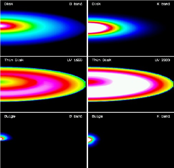
Figure 1: Simulated dust-attenuated images of the disk, thin disk and bulge seen at 78 degrees inclination, for a total central face-on optical depth in the B band $\tau^{\rm f}_{\rm B}=4$. Only the right hand side of each image is displayed, with the centre of the galaxy lying half way along the left hand border of each panel. The dust disks which produce the attenuation are inclined such that they are closer to the observer on the lower half of each image. All images have been displayed with the same spatial scale and have the same colour table. For each pair of images, pixels with the same intensity are displayed with the same colour. Each image was scaled such that the brightest pixel on the corresponding unattenuated image has the value 1.0. In this way one can see the effect of increased opacity with decreasing wavelength, by comparing the left hand panel with the right hand panel, for each geometrical component. The top panels show the disk in the B band (left) and K band (right). The smaller extent of the disk as seen in the K band is due to the smaller scalelength of the stellar emissivity in the K band compared to that in the B band. In both images the maximum brightness comes from the central regions, though at B band the area of bright emission (white colour) is smaller than that in the K band, due to the increased opacity. The middle panels show the thin disk at 1650 $\AA$ (left) and 2800 $\AA$ (right). In both images the maximum brightness is no longer in the central region, but at an intermediate radius, leaving a central “hole”, whose area (red colour) is larger at the shorter UV wavelength. The asymmetry around the horizontal axis is caused by the stronger forward scattering which brightens the near side of the thin disk compared to the far side. The bottom panels show the bulge in the B (left) and K band (right). In the K band bulge emission from both above and below the dust disks is seen, though the emission from below is somewhat attenuated. In the B band almost all the emission from below the dust disk is obscured.

3 Calculation of attenuation in the diffuse component

This section describes the use of radiation transfer calculations to obtain the attenuation in the diffuse component. No radiation transfer calculations are needed for the clumpy component, which is handled analytically (see Sect. 5).

Figure 2: Examples of the dependence of attenuation ($\Delta m$) on inclination ($i$) for the main geometrical components of our model: disk (top left), bulge(top right), and thin disk (bottom left and right). The examples are plotted for the B band for the disk and bulge, and both for the B band and UV 1350$\AA$ for the thin disk. In each panel we plotted (from top to bottom) 7 attenuation curves, corresponding to $\tau^{\rm f}_{\rm B}$: 8, 4, 2, 1, 0.5, 0.3, and 0.1. The face-on orientation corresponds to $1-\cos(i)=0.0$ and the edge-on orientation corresponds to $1-\cos(i)=1.0$.

The basic approach used here is to calculate the attenuation separately for the three diffuse geometrical components of our model: the disk, the thin disk and the bulge. In each case the same fixed geometry of the diffuse dust is adopted, which is the superposition of the dust in the disk and the dust in the thin disk. In other words we derive the attenuation of the old stellar population in the disk as seen through the dust in the disk and thin disk; we derive the attenuation of the young stellar population in the thin disk as seen though the same dust in the disk and thin disk; and we derive the attenuation of the bulge, also viewed through the dust in the disk and thin disk.

The calculations were performed for combinations of the two parameters affecting the diffuse component, $\tau_{\rm B}^{\rm f}$ and inclination $i$. For the sampling in $\tau_{\rm B}^{\rm f}$ we chose the set of values: ${0.1,0.3,0.5,1.0,2.0,4.0,8.0}$ which range from extremely optically thin to moderately optically thick cases. For the sampling in inclination we chose $0\leq\cos(i)\leq 1$, with $\Delta\cos(i)=0.05$. Each calculation was performed at a different wavelength, covering the whole UV/optical/NIR range, such that attenuation can be conveniently calculated for both standard optical bands and the bands covered by GALEX. Our choice of UV wavelengths also samples the 2200 $\AA$ feature. The calculations in the UV range were only performed for the thin disk, since this is the only component of stellar emissivity emitting in this spectral range. In total we used 12 wavelengths, listed in Table 3.

Simulated images of the pure disk, thin disk and bulge were calculated for each combination of parameters using the radiative transfer code of Kylafis & Bahcall (1987), which includes anisotropic multiple scattering. In total we produced 3234 images with a pixel size (equal to the resolution) of 0.0066 of the B-band scalelength $h^{\rm disk}_{\rm s}$, sampled every 5 and 10 pixels in the inner and outer disk, respectively. The high resolution of the simulated images matches the resolution of the optical images of NGC 891 used in the optimisation procedure for the derivation of the disk/bulge geometry. This choice enables not only high accuracy in the derivation of attenuation, but also means that the resulting model images (after suitable interpolation) can be used as template images for comparison with observed images of real galaxies. The simulated images for the disks extend out to a radius of 4.63 B-band scalelengths $h^{\rm disk}_{\rm s}$, which is equivalent to 3.31 dust scalelengths $h^{\rm disk}_{\rm d}$. The simulated images for the bulge extend out to 1.45 B-band scalelength $h^{\rm disk}_{\rm s}$. For both the disks and the bulge the extent of the integration is a numerical limit. Examples of simulated images for the disk, thin disk and bulge are given in Fig. 1.

We also produced the corresponding intrinsic images of the stellar emissivity (as would be observed in the absence of dust). The attenuation ${\Delta}m$ was then obtained by subtracting the integrated magnitude of the dust affected images from the integrated magnitude of the intrinsic images.

At this point we have obtained values of the attenuation for different combinations of $i$ and $\tau^{\rm f}_{\rm B}$, at each wavelength, and independently for the disk, thin disk and bulge. To facilitate access to this information and to allow attenuation to be calculated for any inclination, we fit the attenuation curves (${\Delta}m$ vs $i$) with polynomial functions of the form:

$$\Delta m=\left\{\begin{array}[]{lll}\displaystyle\sum_{{\rm j}=0,n}a_{\rm j}(1-\cos(i))^{\rm j}&{\rm for}&1-\cos(i)\leq 0.90\\ b_{0}&{\rm for}&1-\cos(i)=0.95\\ b_{1}&{\rm for}&1-\cos(i)=1.00\\ \end{array}\right.$$ (9)

where $n=5$ for the disk and thin disk and $n=4$ for the bulge. Values for the coefficients $a_{j}$ and for the constants $b_{0}$ and $b_{1}$ are given in Tables 4, 5 and 6 for the disk, thin disk and bulge, respectively. To derive the attenuation for any desired combination of $i$ and $\tau^{\rm f}_{\rm B}$ one can first apply Eq. 6 to obtain the values of ${\Delta}m$ corresponding to the sampled $\tau^{\rm f}_{\rm B}$ and then interpolate between these values. Subsequently one can also interpolate in wavelength.

It should be noted that slight negative values for $\Delta m$ are obtained for some combinations of low inclination and low $\tau^{\rm f}_{\rm B}$. This mild amplification is due to the scattering of light which removes photons travelling at high inclinations (in the plane of the disk) and sends them into directions with low inclinations, as also shown by Baes & Dejonghe (2001) for the case of isotropic scattering.

In Fig. 2 we show examples of the dependence of attenuation on inclination for the three geometrical diffuse components, both in the optical and in the UV. As expected, the increase in attenuation with increasing inclination is stronger for larger $\tau^{\rm f}_{\rm B}$ than for lower $\tau^{\rm f}_{\rm B}$, irrespective of geometry or wavelength.

4 Attenuation characteristics for the disk, thin disk and bulge

4.1 Attenuation of the disk

In Fig. 3 (upper four panels) we show the wavelength dependence of the attenuation of the disk, from the B band to the K band. As expected, the overall level of the attenuation increases with increasing $\tau^{\rm f}_{\rm B}$. Another feature is the bunching of the curves at low inclinations and low $\tau^{\rm f}_{\rm B}$, followed by an increase in the spacing of the curves when proceeding to higher inclinations and higher $\tau^{\rm f}_{\rm B}$. This can be explained as follows. At low inclination and $\tau^{\rm f}_{\rm B}$ most of the disk is optically thin and the attenuation will scale as $-log(1-\tau)$, where $\tau$ is the line of sight optical depth. Thus, in this regime, changes in inclination or $\tau^{\rm f}_{\rm B}$ induce only small changes in apparent magnitude. However, as we proceed to higher inclinations and $\tau^{\rm f}_{\rm B}$, the disk area which is optically thick will increase from the centre, spreading to the outside. In the inner optically thick part of the disk attenuation scales linearly with $\tau$ whereas in the outer optically thin parts the attenuation still scales logarithmically. Thus the increasing fraction of the disk area which is optically thick will have the effect of inducing bigger and bigger changes in the apparent magnitudes.

Figure 3: The dependence of the attenuation ($\Delta m$) of the disk (upper four panels) and of the bulge (lower four panels) on optical/NIR wavelength ($\lambda$). In each case the panels display the attenuation curves for different $\tau^{\rm f}_{\rm B}$: 0.3, 1, 4 and 8. In each panel the symbols represent attenuations calculated for 5 optical/NIR wavelengths: B, V, I, J and K band. The solid lines represent the linear interpolation between adjacent calculated points. In each panel we plotted (from top to bottom) 8 attenuation curves, corresponding to inclinations $1-\cos(i)$: 1, 0.95, 0.90, 0.85, 0.75, 0.60, 0.40, 0.

The bunching of the curves of attenuation versus wavelength at low inclination and low $\tau^{\rm f}_{\rm B}$ can also be appreciated from examination of the curves of attenuation versus inclination shown in Fig. 2a (for the case of the B band). The bottom curves of Fig. 2a, corresponding to low $\tau^{\rm f}_{\rm B}$, are almost flat over most of the inclination range, meaning that the increase in inclination produces only small changes in attenuation. Similarly, the increase in the spacing of the curves of attenuation versus wavelength at high inclination and high $\tau^{\rm f}_{\rm B}$ from Fig. 3 (upper four panels) is reflected by the upper curves of Fig. 2a (corresponding to high $\tau^{\rm f}_{\rm B}$), which continuously steepen.

A further feature of the disk attenuation is the smaller spacing of the curves between the edge-on geometry and the slightly inclined from edge-on geometry (the two top curves in each of the upper four panels of Fig. 3), an effect which becomes more pronounced at high $\tau^{\rm f}_{\rm B}$. This effect can also be seen in Fig. 2a for the case of the B band, where the curves of attenuation versus inclination flatten when approaching the edge-on viewing angle. This is because the stellar disk has a higher scale height than the dust. In the edge-on view, the high z tail of the stellar population will be visible both above and below the plane. This will tend to boost the apparent luminosity of the disk compared with the slightly inclined disk, partially cancelling the dimming due to the increased line-of-sight optical depth.

4.2 Attenuation of the bulge

Analogous to the case of the disk, we present the wavelength dependence of the attenuation of the bulge in Fig 3 (lower four panels). The most interesting result is the larger overall attenuation of the bulge, as compared to that of the disk (Fig 3, upper four panels). This is because the bulge is more concentrated towards the optically thick part of the dust disks. For the same reason the curves also exhibit a strong dependence of attenuation on inclination. Especially for low $\tau^{\rm f}_{\rm B}$, this dependence is even more pronounced than for the disks. At high $\tau^{\rm f}_{\rm B}$ though, the variation of attenuation with inclination is limited by the larger vertical extent of the stellar population of the bulge compared to the vertical extent of the dust.

Another feature of the attenuation curves for the bulges is the crossing of the two uppermost curves, for 87 and 90 degrees (Fig. 3, lower four panels). The intersection of the curves occurs at a critical wavelength (which depends on $\tau^{\rm f}_{\rm B}$), shortwards of which the highest attenuation is no longer for 90 degrees inclination, but instead at a slightly smaller inclination. This critical wavelength increases with increasing $\tau^{\rm f}_{\rm B}$: it lies between B and V bands for $\tau^{\rm f}_{\rm B}=1$ , between V and I bands for $\tau^{\rm f}_{\rm B}=2$, between I and J bands for $\tau^{\rm f}_{\rm B}=4$ and goes to K band for $\tau^{\rm f}_{\rm B}=8$. The explanation for these features is as follows. If we consider that the dust disk is optically thick for all lines of sight intersecting the bulge, then the fraction of light blanked out is simply proportional to the projected area of the disk onto the bulge. Since the projected area of the disk is at a minimum for an inclination of 90 degrees, moving away from the edge-on geometry will increase the attenuation. If we progress to even lower inclinations the disk will start to become optically thin for some lines of sight through the bulge, and then the attenuation will start to decrease with decreasing inclination. This non-monotonic progression of attenuation with inclination close to the edge-on orientation is also illustrated in Fig. 2b (for the example of the B band). There one can see that the maximum attenuation is no longer reached at 90 degrees for $\tau^{\rm f}_{\rm B}\geq 1$.

Figure 4: The dependence of the attenuation ($\Delta m$) of the thin disk on UV wavelength (upper four panels) and on optical/NIR wavelength (lower four panels). Curves are plotted as in Fig. 3, except that for the upper four panels the symbols now represent attenuations calculated for 7 UV wavelengths: 912, 1350, 1650, 2000, 2200, 2500 and 2800 $\AA$.

4.3 Attenuation of the thin disk

In Fig. 4 (upper four panels) we show the dependence of the attenuation of the thin disk on UV wavelength. In this wavelength range the opacity does not decrease monotonically with increasing wavelength, as it does in the optical regime, because of the local maximum around 2200 $\AA$ in the extinction efficiencies. This causes the bump around 2200 $\AA$ seen in the attenuation curves in Fig. 4 (upper four panels).

As in the case of the attenuation of the disk (Fig. 3, upper four panels), one can observe a bunching of the curves for low inclinations and low $\tau^{\rm f}_{\rm B}$, followed by an increase in the spacing between curves in proceeding to high inclinations and high $\tau^{\rm f}_{\rm B}$. In addition to the factors contributing to this effect discussed in Sect. 4.1, scattering of light also payes a role. Photons travelling at high inclinations (in the plane of the disk) are scattered into directions with low inclinations, such that they can escape the disk (as explained by Baes & Dejonghe 2001 for the case of isotropic scattering). This factor also influences the attenuation in the disk, but is more important in the case of the thin disk, since here the stars have a stronger correlation with the dust, so that the contrast between the edge-on and the face-on optical depth is higher.

Figure 5: Comparison between the attenuation curves of the disk, thin disk and bulge. The 4 panels show the dependence of the attenuation on optical wavelength, for 4 inclinations: 0, 60, 87 and 90 degrees, and for the same $\tau^{\rm f}_{\rm B}=4$. In each panel the attenuation for the disk, thin disk and bulge are plotted with solid, dashed and dotted lines, respectively.

At high $\tau^{\rm f}_{\rm B}$, however, there is a small tendency for the curves for the edge-on and nearly edge-on inclinations to come together. This effect, which is most prominent for 912 $\AA$ and $\tau^{\rm f}_{\rm B}=8$ (Fig. 4, upper four panels), is primarily a saturation effect due to the fact that only a thin skin is seen close to edge-on.

In Fig. 4 (lower four panels) we show the dependence of the attenuation of the thin disk on optical wavelength. At larger inclinations, the thin disk exhibits the largest attenuation in the optical range, as compared with the disk and the bulge. This is because of the strong spatial correlation between the stars and the dust. For the same reason, the thin disk also exhibits the strongest dependence on inclination. Despite the larger attenuation, the contribution of this geometrical component to the overall attenuation of the galaxy in the optical range is small and can be neglected, since the thin disk emits mainly in the UV. However the attenuation of the thin disk in the optical range is important for the calculation of optical line emission arising from the thin disk.

4.4 Intercomparison of the attenuations of the disk, thin disk and bulge

In the previous subsections we described and discussed the main characteristics of the attenuation curves of the main geometrical components of our model, namely of the disk, thin disk and the bulge. To make an intercomparison of the curves for the different geometries we superpose in Fig. 5 attenuation curves for the three geometrical components, for the same inclination and $\tau^{\rm f}_{\rm B}$. The value of $\tau^{\rm f}_{\rm B}$ was chosen to be 4, which, for the geometry of our model, is close to what we found for NGC 891.

At low and intermediate inclinations the bulge suffers a larger attenuation than that of the disk or thin disk (Fig. 5a,b). As already noted, this is because the bulge is more concentrated towards the optically thick part of the dust disks. In addition, and for the same reason, the figure also shows that the attenuation of the bulge has the steepest dependence on optical wavelength. It is also apparent from Fig. 5a,b that the attenuation curves for the disk and thin disk show quite similar behaviour to each other, indicating that at low and intermediate inclinations the curves are not sensitive to the differences in scale height and scale length between the two disks. There is nevertheless a small difference between the curves for the disk and thin disk, in the sense that the thin disk suffers slightly less attenuation, except for the B band. This is because the disk has smaller scale lengths for the stellar population than the thin disk, except for the B band, where the scale length is the same.

With increasing line of sight optical depth, which is the same as increasing inclination and/or decreasing wavelength, the attenuation curve for the thin disk starts to diverge from that of the disk (Fig 5c); it will increase until it intersects with the attenuation curve for the bulge. This is because the thin disk has the smallest scale height, the strongest spatial correlation with the dust and the largest contrast between the face-on and edge-on orientation, and so its attenuation depends most strongly on inclination (or wavelength). So for edge-on orientation (Fig. 5d) the attenuation of the thin disk dominates that of the other geometrical components, reversing the situation for the face-on orientation (Fig. 5a), where the thin disk has the smallest attenuation.

5 Composite attenuation curves for spiral galaxies

Spiral galaxies have varying proportions of their stellar luminosities emitted by the disk, thin disk and bulge and also varying amounts of clumpiness. For instance the bulge-to-disk ratio decreases in going from earlier to later spiral types (see for example Fig. 7 of Trujillo et al. 2002). In the previous sections we have calculated attenuation curves quantifying the extinction of the individual stellar populations from the disk, thin disk and bulge due to the diffuse dust. These can be combined to obtain a composite attenuation curve for the light illuminating the diffuse dust in a galaxy. If we also consider the photons that don’t reach the diffuse dust because they are absorbed by the clumpy dust, local to the star-forming regions, then we obtain the composite attenuation curve for the total luminosity of the galaxy.

5.1 A formula to calculate composite attenuations

At a given wavelength $\lambda$, the total attenuation ${\Delta}m_{\lambda}$ in a galaxy is given by:

$${\Delta}m_{\lambda} = -2.5\log\frac{S_{\lambda}}{S^{\rm 0}_{\lambda}},$$ (10)

where $S^{\rm 0}_{\lambda}$ and $S_{\lambda}$ are the intrinsic and the apparent flux densities, respectively. The quantities $S^{\rm 0}_{\lambda}$ and $S_{\lambda}$ can be further expressed as a summation of the corresponding quantities for the disk, thin disk and bulge:

$$S^{\rm 0}_{\lambda} = S^{\rm 0,disk}_{\lambda}+S^{\rm 0,tdisk}_{\lambda}+S^{\rm 0,bulge}_{\lambda}$$ (11)

$$S_{\lambda} = S^{\rm disk}_{\lambda}+S^{\rm tdisk}_{\lambda}+S^{\rm bulge}_{\lambda}.$$ (12)

The apparent and intrinsic flux densities for the disk, thin disk and bulge are related as follows:

$$S^{\rm 0,disk}_{\lambda} = S^{\rm disk}_{\lambda}\,10^{\frac{\displaystyle{\Delta}m^{\rm disk}_{\lambda}}{\displaystyle 2.5}}$$ (13)

$$S^{\rm 0,tdisk}_{\lambda} = \frac{S^{\rm tdisk}_{\lambda}}{1-F\,f_{\lambda}}10^{\frac{\displaystyle{\Delta}m^{\rm tdisk}_{\lambda}}{\displaystyle 2.5}}$$ (14)

$$S^{\rm 0,bulge}_{\lambda} = S^{\rm bulge}_{\lambda}\,10^{\frac{\displaystyle{\Delta}m^{\rm bulge}_{\lambda}}{\displaystyle 2.5}},$$ (15)

where ${\Delta}m^{\rm disk}_{\lambda}$, ${\Delta}m^{\rm tdisk}_{\lambda}$ and ${\Delta}m^{\rm bulge}_{\lambda}$ are the attenuation values for the disk, thin disk and bulge, which can be derived from Tables 4-6, F is the clumpiness factor as defined in Sect. 2.2 and $f_{\lambda}$ is the function defined in Appendix A and tabulated in Table A.1. In physical terms, $F\,f_{\lambda}$ is the fraction of the emitted UV flux density at wavelength $\lambda$ which is locally absorbed in star-forming regions.

If we define the ratios of the apparent luminosities of disk, thin disk and bulge to the total apparent luminosity to be:

$$r^{\rm disk}_{\lambda} = \frac{S^{\rm disk}_{\lambda}}{S_{\lambda}}$$ (16)

$$r^{\rm tdisk}_{\lambda} = \frac{S^{\rm tdisk}_{\lambda}}{S_{\lambda}}$$ (17)

$$r^{\rm bulge}_{\lambda} = \frac{S^{\rm bulge}_{\lambda}}{S_{\lambda}},$$ (18)

then the total attenuation of the galaxy can be expressed as:

$${\Delta}m_{\lambda} = 2.5\log(r^{\rm disk}_{\lambda}\,10^{\frac{\displaystyle{\Delta}m^{\rm disk}_{\lambda}}{\displaystyle 2.5}}$$

$$\leavevmode\nobreak\ \leavevmode\nobreak\ \leavevmode\nobreak\ \leavevmode\nobreak\ \leavevmode\nobreak\ \leavevmode\nobreak\ \leavevmode\nobreak\ \leavevmode\nobreak\ +\,\frac{1-r^{\rm disk}_{\lambda}-r^{\rm bulge}_{\lambda}}{1-F\,f_{\lambda}}\,10^{\frac{\displaystyle{\Delta}m^{\rm tdisk}_{\lambda}}{\displaystyle 2.5}}$$

$$\leavevmode\nobreak\ \leavevmode\nobreak\ \leavevmode\nobreak\ \leavevmode\nobreak\ \leavevmode\nobreak\ \leavevmode\nobreak\ \leavevmode\nobreak\ \leavevmode\nobreak\ +\,r^{\rm bulge}_{\lambda}\,10^{\frac{\displaystyle{\Delta}m^{\rm bulge}_{\lambda}}{\displaystyle 2.5}}).$$ (19)

This is a general formula giving the composite attenuation curve as a function of 5 independent parameters: $i$, $\tau^{\rm f}_{\rm B}$, $r^{\rm disk}_{\lambda}$, $r^{\rm bulge}_{\lambda}$ and $F$. For practical application, this formula can be simplified if we write it separately for the UV and the optical/NIR ranges. It is a good approximation to consider that the thin disk emits only in the UV range and the disk and bulge only in the optical/NIR range. This approximation has been validated by our detailed analysis on NGC 891 in Paper I. In the UV Eq. 16 becomes:

$${\Delta}m^{\rm UV}_{\lambda} = {\Delta}m^{\rm tdisk}_{\lambda}-2.5\log(1-F\,f_{\lambda}),$$ (20)

while in the optical/NIR Eq. 16 becomes:

$${\Delta}m^{\rm optical}_{\lambda} = 2.5\log((1-r^{\rm bulge}_{\lambda})\,10^{\frac{\displaystyle{\Delta}m^{\rm disk}_{\lambda}}{\displaystyle 2.5}}$$

$$\leavevmode\nobreak\ \leavevmode\nobreak\ \leavevmode\nobreak\ \leavevmode\nobreak\ \leavevmode\nobreak\ \leavevmode\nobreak\ \leavevmode\nobreak\ \leavevmode\nobreak\ +\,r^{\rm bulge}_{\lambda}\,10^{\frac{\displaystyle{\Delta}m^{\rm bulge}_{\lambda}}{\displaystyle 2.5}}).$$ (21)

5.2 Choice of parameter values

Both Eqs. 17 and 18 have three free parameters: ${\tau}^{\rm f}_{\rm B}$, $i$ and $F$ for the UV range and ${\tau}^{\rm f}_{\rm B}$, $i$ and $r^{\rm bulge}_{\lambda}$ for the optical/NIR range.

For resolved objects, the apparent bulge-to-total luminosity ratio $r^{\rm bulge}_{\rm\lambda}$ can be derived directly from observations, by decomposing the bulge from the disk.

A realistic derivation of the $F$ factor requires a complete modelling of the whole UV-submm SED. Another approach would be to derive the $F$ factor directly from comparing highly resolved FIR images with images in the UV, which soon may become feasible with the advent of GALEX in conjunction with ISO and future SIRTF observations of nearby galaxies. For a simple recipe, the median value of the $F$ factors derived in Paper II can be used, namely $F=0.22$, which is also the value obtained for NGC 891. We note here that it cannot be ruled out that $F$ may increase with $SFR$, as suggested by the study of the FIR/radio correlation by Pierini et al. (2003). Physically, this might be expected if an increased SFR is accompanied not only by an increase in the number of independent HII regions, but also by a higher probability for further star formation to happen preferentially near already existing HII regions. Then, the $F$ factor would also increase, as a consequence of the increased blocking capability of the optically thick molecular clouds in the star-forming complex. This would be expected to occur if star formation is a self propagating phenomenon, in which preceding generations of stars can trigger the formation of new generations.

The values of opacities ${\tau}^{\rm f}_{\rm B}$ are also best found from a complete modelling of the whole UV-submm SED. In a companion paper we will present a grid of calculations for the FIR/submm emission corresponding to the attenuations presented in Tables 4-6, from which ${\tau}^{\rm f}_{\rm B}$ can be extracted from a self-consistent fit to the entire UV-submm range. In the absence of FIR photometry, an alternative method to derive ${\tau}^{\rm f}_{\rm B}$ would be to use the emission from the Balmer recombination lines, integrated over the whole galaxy. In our model the emission from these lines arises from the thin stellar disk. These lines will be attenuated both by the diffuse dust (associated with both the young and old stellar populations) and by the clumpy dust (associated with the star-forming regions). Since in the formulation of our model the fraction of the emission locally absorbed in the clumpy component is the same for all lines in the Balmer series, the line ratio will depend only on the attenuation by the diffuse dust. This attenuation can readily be found by interpolating in wavelength between the attenuation values for the thin disk derived from Table 5. As an example, the ratio ${\rm H}\alpha/{\rm H}\beta$ was derived by interpolating in wavelength between the adjacent optical bands to the wavelength of the recombination lines. To present the line ratio in an analogous way to the information from Tables 4-6, we fitted the $\log({\rm H}\alpha/{\rm H}\beta)$ with a 5th order polynomial function of the form:

$$\frac{{\rm H}\alpha}{{\rm H}\beta}=\left\{\begin{array}[]{lll}\displaystyle\sum_{{\rm j}=0,n}a_{\rm j}(1-\cos(i))^{\rm j}&{\rm;}&1-\cos(i)\leq 0.90\\ b_{0}&{\rm;}&1-\cos(i)=0.95\\ b_{1}&{\rm;}&1-\cos(i)=1.00\\ \end{array}\right.$$ (25)

where $n=4$. Values for the coefficients $a_{j}$ and for the constants $b_{0}$ and $b_{1}$ are given in Table 7 and the dependence of the ${\rm H}\alpha/{\rm H}\beta$ line ratio on inclination and ${\tau}^{\rm f}_{\rm B}$ is shown in Fig. 6. If a measurement of the line ratio ${\rm H}\alpha/{\rm H}\beta$ were available for a galaxy of known inclination, this could be compared with the calculated ratios derived from Table 7 to derive ${\tau}^{\rm f}_{\rm B}$.

Figure 6: The effect of dust on the ${\rm H}\alpha/{\rm H}\beta$ line ratio as a function of inclination $i$. The seven curves (from top to bottom) correspond to $\tau^{\rm f}_{\rm B}$: 8, 4, 2, 1, 0.5, 0.3, and 0.1. The face-on orientation corresponds to $1-\cos(i)=0.0$ and the edge-on orientation corresponds to $1-\cos(i)=1.0$.

Table 7: Coefficients and constants for the calculation of the ${\rm H}\alpha/{\rm H}\beta$ line ratio

$\tau^{\rm f}_{\rm B}$	$a_{0}$	$a_{1}$	$a_{2}$	$a_{3}$	$a_{4}$	$b_{0}$	$b_{1}$
0.1	2.732	-0.062	0.472	-0.989	0.711	2.853	3.152
0.3	2.740	-0.118	0.716	-1.477	1.181	3.030	3.419
0.5	2.751	-0.159	0.963	-1.967	1.629	3.155	3.525
1.0	2.779	-0.237	1.421	-2.638	2.155	3.357	3.660
2.0	2.833	-0.167	1.721	-3.207	2.619	3.605	3.791
4.0	2.977	-0.044	1.945	-3.728	2.988	3.904	3.918
8.0	3.196	-0.042	2.435	-4.730	3.709	4.227	4.018

5.3 An example

To illustrate solutions derived from Eqs. 17-18, we calculate composite attenuation curves for NGC 891 as would be obtained for different inclinations. For this galaxy ${\tau}^{\rm f}_{\rm B}=4.2$ and $F=0.22$ (see Paper I). In this particular case the apparent bulge-to-total ratio $r^{\rm bulge}_{\lambda}$ can be derived from a known intrinsic value (0.246, averaged over the optical/NIR; Xilouris et al. 1999) by application of Eqns. 10 and 12 for the wavelengths and inclinations of interest. Using the values tabulated in Tables 4-6 we obtained the curves plotted in Fig. 7 for three inclinations: 0, 60 and 90 degrees. The curves show a smooth progression with wavelength, except for the edge-on orientation, where there is a steep step between optical and UV, due to the large contrast in attenuation between the thin and thick disks viewed edge-on.

Using the attenuation curve for NGC 891 ($i=89.8^{\circ}$) and the intrinsic flux densities from Paper I we can predict the apparent magnitude of the galaxy in the UV and compare this prediction with observations. Until now the galaxy has been detected only at 2500 $\AA$ by Marcum et al. (2001) who measured $m^{2500}=13.00\pm 0.23$. Our prediction is $m^{2500}=13.29$, in good agreement with the observations, thus reinforcing the validity of the model for the intrinsic stellar luminosity and attenuation presented in Paper I.

Figure 7: Composite attenuation curves for the galaxy NGC 891, as would be obtained if the galaxy were viewed at inclinations of 0, 60 and 90 degrees. $\tau^{\rm f}_{\rm B}=4.2$ and $F=0.22$.

6 The effect of the bulge-to-disk ratio on the derived opacities

To illustrate the use of composite attenuation curves in the interpretation of optical/NIR data we consider the effect of a varying bulge-to-disk ratio on the inclination dependence of the apparent optical emission from galaxies. Traditionally, astronomers have used this dependence to make statistical estimates of the opacity of galaxian disks through analysis of large samples of spiral galaxies. But these studies have not taken into account the fact that the attenuation of the bulge has a different variation with inclination than that of the disk, as shown in Sect. 4.

In order to quantify the effect of the bulge-to-disk ratio on the derived opacities, we calculated the variation of the composite attenuation with inclination for three different opacities, $\tau^{\rm f}_{\rm B}=2,4,8$. These curves were calculated for a grid of values of the bulge-to-disk ratio ranging from 0 to 100, which represent the whole range between “pure disk” and “pure bulge” galaxies. We chose to do these calculations in the K band in order to compare our results with recent statistical studies of internal extinction in spiral galaxies in the NIR. For a convenient comparison with observational studies we fitted the variation of the composite attenuation with -$\log(\cos(i))$ using a linear fit to the lower inclination range ($1-\cos(i)<0.7$). The resulting slope of the fit $\gamma_{\rm K}$ is plotted in Fig. 8 versus the bulge-to-disk ratio and for the 3 opacities considered. All curves show a “S-like” shape, tending towards the asymptotes of the “pure” disk and “pure” bulge. It can be seen from Fig. 8 that an increase from 0 to 1 in bulge-to-disk ratio (which embraces the observed range; Trujillo et al. 2002) produces a comparable change in $\gamma_{\rm K}$ to that resulting from a doubling of the opacity of a “pure” disk. For example, changing the bulge-to-disk ratio from 0 to 1 for $\tau^{\rm f}_{\rm B}=2$ increases $\gamma_{\rm K}$ by a factor of 2.2, whereas increasing the opacity from $\tau^{\rm f}_{\rm B}=2$ to 4 changes $\gamma_{\rm K}$ by a factor of only 1.9 for a “pure” disk galaxy. Thus, increasing the bulge-to-disk ratio at a constant opacity can mimic the effect of increasing the opacity of a “pure” disk.

Figure 8: The slope $\gamma_{\rm K}$ versus the intrinsic bulge-to-disk ratio, where $\gamma_{\rm K}$ is the slope of a linear fit to the low inclination part ($1-\cos(i)<0.7$) of the composite attenuation curve (${\Delta}$m vs -$\log(\cos(i)$)) in the K band. The calculations were performed for $\tau^{\rm f}_{\rm B}=8,4,2$.

This may have consequences for the use of optical statistical samples to evaluate the dependence of opacity on galaxy luminosity. For example, in their study of 15224 spiral galaxies from the 2 Micron All-Sky Survey, Masters et al. (2003) found a trend for the slope $\gamma_{\rm K}$ (and also for the corresponding slopes in J and H bands) to increase with increasing K-band luminosity. These authors interpret this result as a trend of increasing disk opacity with increasing K-band luminosity. However, galaxies that have brighter K-band luminosities are also biased towards earlier-type spirals (e.g. Boselli et al. 1997), which in turn have larger bulge-to-disk ratios. Fig. 13 of Masters et al. (2003) show a variation of 0.2 in $\gamma_{\rm K}$ over the luminosity range of their sample, which is comparable to the variation in $\gamma_{\rm K}$ found in our Fig. 8 between bulge-to-disk ratios of 0 and 1. This raises the possibility that some of the trend found by Masters et al. (2003) is due to a systematic increase in the bulge-to-disk ratio with luminosity in their sample. It will be important to quantify this effect in studies that investigate the dependence of the ratio of the FIR luminosity to the intrinsic UV luminosity of gas rich galaxies on the stellar mass of the galaxies (Pierini & Möller 2003). In general, ignoring the presence of bulges can lead to a systematic overestimate of the opacity of disks.

7 Summary and conclusions

We present new calculations for the attenuation of the integrated stellar light from spiral galaxies, utilising geometries for stars and dust constrained by a joint consideration of the UV/optical and FIR/submm SEDs. In addition to the single exponential diffuse dust disk used in previous studies of attenuation, we also invoke a clumpy and strongly heated distribution of grains spatially correlated with the star-forming regions (required to account for the FIR colours) and diffuse dust associated with the spiral arms (needed to account for the amplitude of the submm emission). The latter is approximated by a second exponential dust disk having the same spatial distribution as the young, UV emitting stellar population, also approximated by an exponential disk - the “thin disk”. The old, optical/NIR-emitting stellar population is specified by an exponential disk of larger scale height - the “disk”, plus a de Vaucouleurs bulge - the “bulge”.

Radiation transfer calculations were performed separately for the three diffuse emissivity components (disk, thin disk and bulge) seen through the same fixed distribution of diffuse dust. We used the radiative transfer code of Kylafis & Bahcall (1987) which includes anisotropic multiple scattering. The attenuation of each component was calculated for a grid of central face-on B-band optical depth $\tau^{\rm f,disk}_{\rm B}$ and inclination $i$, for a range of wavelengths from 912 $\AA$ to 2.2 ${\mu}$m. The resulting curves of attenuation versus inclination were fitted with polynomial function and the coefficients tabulated in Tables 4-6. The tables allow the attenuation to be obtained for any desired combination of $\tau^{\rm f,disk}_{\rm B}$, $i$, and wavelength, by interpolation in $\tau^{\rm f,disk}_{\rm B}$ and wavelength.

The clumpy component was handled analytically, whereby the wavelength dependence of local absorption of starlight in star-forming regions was purely determined from geometrical considerations. By combining the global attenuation of the individual stellar populations from the disk, thin disk and bulge due to the diffuse dust with the local attenuation due to the clumpy dust associated with the star-forming regions, we obtain a general formula for the calculation of composite attenuation of the integrated emission from spiral galaxies. As an example of this formula, we calculated composite attenuation curves for NGC 891 as would be seen at different inclinations. Using the attenuation curve for NGC 891 at the actual inclination $i=89.8^{\circ}$ we predicted the apparent magnitude of this galaxy in the UV and found this prediction to be in good agreement with the recent observations of Marcum et al. (2001).

We also used our model to derive the ratio ${\rm H}\alpha/{\rm H}\beta$ as a function of inclination and $\tau^{\rm f}_{\rm B}$. This information is presented in Table 7 in form of polynomial fits and can be used to derive the value of $\tau^{\rm f}_{\rm B}$ for objects with no FIR/submm photometry.

The detailed analysis of the attenuation properties of the individual geometrical components led to the following conclusions:

• For a typical galaxy and in the optical/NIR spectral range, the relative attenuation between the disk, thin disk and bulge depends strongly on inclination. At low and intermediate inclinations, the bulge suffers a larger attenuation than that of the disk or thin disk, and has the steepest dependence on wavelength. Furthermore, in this regime, the curves of attenuation versus wavelength for the disk and thin disk show quite similar behaviour to each other, indicating that the attenuation is not sensitive to the differences in scale height and scale length between the two disks. At higher inclinations, however, the attenuation curves for the thin disk start to diverge from those of the disk. For the edge-on orientation the attenuation of the thin disk dominates that of the other geometrical components, reversing the situation for the face-on orientation, where the thin disk has the smallest attenuation.

• Increasing the bulge-to-disk ratio at a constant opacity can mimic the effect of increasing the opacity of a “pure” disk. In general, ignoring the presence of bulges can lead to a systematic overestimate of the opacity of disks.

Table 4: Coefficients and constants for the calculation of the attenuation of the disk

$\tau^{\rm f}_{\rm B}$	$a_{0}$	$a_{1}$	$a_{2}$	$a_{3}$	$a_{4}$	$a_{5}$	$b_{0}$	$b_{1}$
B band
0.1	-0.002	0.069	-0.725	2.645	-3.883	2.107	0.163	0.240
0.3	-0.003	0.038	-0.458	2.528	-4.536	2.935	0.390	0.483
0.5	0.008	0.055	-0.785	3.964	-6.569	4.037	0.544	0.632
1.0	0.022	0.210	-1.352	5.519	-8.182	4.799	0.795	0.874
2.0	0.083	0.321	-1.493	6.148	-8.757	5.039	1.086	1.165
4.0	0.215	0.491	-1.878	7.473	-10.356	5.757	1.414	1.505
8.0	0.432	0.635	-2.166	8.304	-11.297	6.189	1.783	1.892
V band
0.1	-0.005	0.060	-0.636	2.303	-3.346	1.786	0.124	0.191
0.3	-0.006	0.033	-0.462	2.371	-4.125	2.596	0.317	0.408
0.5	-0.002	0.046	-0.628	3.265	-5.552	3.463	0.456	0.544
1.0	0.007	0.125	-0.884	4.200	-6.720	4.158	0.689	0.769
2.0	0.048	0.229	-1.048	4.815	-7.218	4.378	0.966	1.040
4.0	0.148	0.406	-1.518	6.391	-9.025	5.149	1.281	1.361
8.0	0.333	0.582	-1.996	7.855	-10.787	5.947	1.632	1.730
I band
0.1	-0.006	0.033	-0.385	1.515	-2.289	1.239	0.080	0.130
0.3	-0.005	0.063	-0.752	2.996	-4.546	2.535	0.223	0.306
0.5	-0.005	0.056	-0.718	3.215	-5.139	3.025	0.336	0.424
1.0	-0.002	-0.029	0.164	1.111	-3.019	2.460	0.541	0.621
2.0	0.018	0.046	0.087	1.456	-3.303	2.690	0.797	0.864
4.0	0.077	0.201	-0.224	2.368	-4.028	2.925	1.092	1.156
8.0	0.210	0.427	-0.931	4.499	-6.498	3.975	1.422	1.497
J band
0.1	-0.004	0.020	-0.237	0.924	-1.353	0.699	0.038	0.065
0.3	-0.004	0.015	-0.245	1.300	-2.241	1.329	0.119	0.177
0.5	-0.004	0.001	-0.121	1.144	-2.308	1.529	0.190	0.264
1.0	-0.002	0.023	-0.234	1.835	-3.541	2.347	0.339	0.420
2.0	0.008	0.074	-0.409	2.667	-4.827	3.189	0.551	0.620
4.0	0.038	0.134	-0.335	2.571	-4.564	3.173	0.814	0.865
8.0	0.112	0.252	-0.362	2.655	-4.250	2.934	1.115	1.159
K band
0.1	-0.003	0.024	-0.256	0.832	-1.037	0.452	0.009	0.018
0.3	-0.001	0.033	-0.357	1.266	-1.744	0.856	0.039	0.065
0.5	0.000	0.038	-0.433	1.622	-2.336	1.200	0.068	0.107
1.0	0.006	-0.045	0.185	0.138	-0.903	0.787	0.137	0.196
2.0	0.013	-0.003	-0.096	1.225	-2.544	1.724	0.256	0.329
4.0	0.029	0.055	-0.407	2.446	-4.369	2.801	0.441	0.508
8.0	0.063	0.124	-0.545	3.010	-5.097	3.309	0.688	0.731

Table 5: Coefficients and constants for the calculation of the attenuation of the thin disk

$\tau^{\rm f}_{\rm B}$	$a_{0}$	$a_{1}$	$a_{2}$	$a_{3}$	$a_{4}$	$a_{5}$	$b_{0}$	$b_{1}$
UV 912
0.1	0.046	0.226	-2.242	9.055	-14.193	8.142	0.884	1.677
0.3	0.164	0.219	-3.191	15.257	-24.502	14.129	1.719	2.622
0.5	0.235	0.353	-2.841	14.431	-23.840	14.305	2.228	3.120
1.0	0.440	0.445	-2.370	14.574	-25.276	15.771	3.044	3.843
2.0	0.773	0.509	-1.292	12.835	-24.355	16.239	3.979	4.604
4.0	1.250	0.450	1.412	5.345	-15.012	12.461	4.973	5.379
8.0	1.891	0.165	6.978	-12.176	9.259	0.833	5.956	6.136
UV 1350
0.1	-0.001	0.165	-1.593	6.421	-10.241	5.876	0.532	1.198
0.3	0.057	0.246	-3.086	13.069	-20.582	11.719	1.158	2.022
0.5	0.095	0.272	-3.018	13.642	-21.967	12.875	1.566	2.467
1.0	0.197	0.351	-2.862	14.467	-23.967	14.492	2.244	3.131
2.0	0.396	0.453	-2.434	14.793	-25.590	16.012	3.065	3.852
4.0	0.730	0.627	-1.623	13.302	-24.661	16.376	4.000	4.610
8.0	1.226	0.574	1.049	5.861	-15.294	12.527	4.989	5.377
UV 1650
0.1	-0.011	0.149	-1.426	5.731	-9.137	5.209	0.434	1.044
0.3	0.030	0.264	-3.064	12.364	-19.204	10.828	0.984	1.820
0.5	0.061	0.249	-3.109	13.590	-21.632	12.502	1.356	2.244
1.0	0.131	0.313	-2.979	14.358	-23.483	14.044	1.981	2.882
2.0	0.289	0.430	-2.806	15.516	-26.151	15.996	2.752	3.582
4.0	0.579	0.579	-2.043	14.310	-25.701	16.608	3.649	4.327
8.0	1.022	0.545	0.171	8.751	-19.373	14.399	4.624	5.089
UV 2000
0.1	-0.012	0.114	-1.051	4.721	-8.055	4.873	0.510	1.163
0.3	0.032	0.249	-2.938	12.319	-19.339	11.043	1.116	1.974
0.5	0.067	0.246	-3.087	14.072	-22.503	13.052	1.514	2.413
1.0	0.151	0.321	-2.833	14.546	-24.011	14.433	2.179	3.068
2.0	0.337	0.462	-2.345	14.461	-25.125	15.748	2.985	3.783
4.0	0.671	0.587	-1.559	13.289	-24.689	16.342	3.909	4.537
8.0	1.158	0.498	1.246	5.691	-15.410	12.644	4.892	5.300
UV 2200
0.1	-0.001	0.128	-1.131	4.768	-7.887	4.745	0.550	1.217
0.3	0.042	0.201	-2.522	11.297	-18.234	10.643	1.177	2.041
0.5	0.077	0.222	-2.732	13.130	-21.415	12.632	1.584	2.485
1.0	0.168	0.310	-2.513	13.748	-23.141	14.120	2.263	3.147
2.0	0.367	0.467	-2.108	13.864	-24.484	15.536	3.082	3.867
4.0	0.716	0.590	-1.304	12.625	-23.923	16.059	4.014	4.623
8.0	1.219	0.476	1.751	4.159	-13.387	11.725	4.999	5.387
UV 2500
0.1	-0.023	0.096	-0.875	3.768	-6.313	3.823	0.427	1.029
0.3	-0.003	0.190	-2.169	9.372	-15.179	8.955	0.965	1.796
0.5	0.021	0.169	-2.675	12.596	-20.429	11.943	1.329	2.215
1.0	0.072	0.261	-2.558	13.424	-22.410	13.552	1.947	2.845
2.0	0.227	0.404	-2.272	13.850	-24.035	15.039	2.706	3.538
4.0	0.519	0.523	-1.650	13.389	-24.671	16.153	3.593	4.281
8.0	0.959	0.498	0.462	8.085	-18.634	14.064	4.560	5.034
UV 2800
0.1	-0.015	0.080	-0.629	2.847	-5.000	3.131	0.374	0.931
0.3	0.002	0.168	-2.048	8.843	-14.342	8.419	0.859	1.663
0.5	0.022	0.153	-2.733	12.578	-20.239	11.694	1.197	2.068
1.0	0.056	0.231	-2.705	13.627	-22.465	13.406	1.776	2.678
2.0	0.178	0.373	-2.466	14.133	-24.140	14.899	2.499	3.354
4.0	0.433	0.512	-2.043	14.237	-25.446	16.286	3.353	4.085
8.0	0.832	0.517	-0.276	10.148	-21.226	15.131	4.305	4.838

Table 5: Coefficients and constants for the calculation of the attenuation of the thin disk; Continued

$\tau^{\rm f}_{\rm B}$	$a_{0}$	$a_{1}$	$a_{2}$	$a_{3}$	$a_{4}$	$a_{5}$	$b_{0}$	$b_{1}$
B band
0.1	-0.022	0.116	-1.307	4.915	-7.267	3.833	0.222	0.648
0.3	-0.016	0.215	-2.555	10.182	-15.666	8.567	0.571	1.281
0.5	-0.011	0.257	-3.157	12.891	-19.959	11.044	0.843	1.647
1.0	0.009	0.275	-3.578	15.768	-24.929	14.110	1.320	2.207
2.0	0.060	0.272	-2.665	13.784	-22.905	13.793	1.939	2.837
4.0	0.217	0.411	-2.356	14.142	-24.442	15.240	2.700	3.530
8.0	0.509	0.508	-1.581	13.298	-24.657	16.184	3.587	4.272
V band
0.1	-0.018	0.092	-0.954	3.339	-4.755	2.484	0.166	0.517
0.3	-0.014	0.168	-1.901	7.380	-11.288	6.205	0.444	1.086
0.5	-0.013	0.215	-2.539	10.169	-15.695	8.702	0.677	1.429
1.0	-0.004	0.246	-3.052	13.207	-20.914	11.885	1.101	1.958
2.0	0.027	0.226	-2.625	13.023	-21.412	12.766	1.656	2.559
4.0	0.129	0.358	-2.437	13.748	-23.386	14.396	2.356	3.226
8.0	0.363	0.501	-2.060	13.957	-24.816	15.836	3.191	3.951
I band
0.1	-0.015	0.099	-1.028	3.483	-4.774	2.360	0.099	0.342
0.3	-0.013	0.098	-1.013	4.142	-6.653	3.789	0.281	0.794
0.5	-0.017	0.161	-1.688	6.837	-10.763	6.030	0.451	1.092
1.0	-0.018	0.233	-2.399	10.019	-15.881	9.012	0.784	1.569
2.0	-0.010	0.262	-2.517	11.241	-18.131	10.659	1.245	2.121
4.0	0.041	0.317	-2.517	12.639	-20.955	12.677	1.838	2.741
8.0	0.175	0.424	-2.166	13.041	-22.622	14.197	2.575	3.426
J band
0.1	-0.013	0.061	-0.619	2.041	-2.712	1.296	0.040	0.166
0.3	-0.005	0.072	-0.811	3.134	-4.751	2.534	0.121	0.442
0.5	-0.006	0.092	-1.037	4.158	-6.450	3.525	0.215	0.655
1.0	-0.007	0.132	-1.510	6.434	-10.262	5.739	0.420	1.036
2.0	-0.001	0.087	-1.678	8.377	-13.945	8.065	0.742	1.510
4.0	0.019	0.172	-2.137	10.787	-18.017	10.624	1.195	2.062
8.0	0.076	0.266	-2.252	12.197	-20.669	12.506	1.778	2.683
K band
0.1	-0.012	0.071	-0.675	1.983	-2.340	0.982	0.004	0.051
0.3	-0.001	0.036	-0.399	1.470	-2.152	1.094	0.018	0.158
0.5	0.000	0.071	-0.753	2.703	-3.856	1.926	0.051	0.255
1.0	0.002	0.112	-1.182	4.298	-6.185	3.141	0.132	0.463
2.0	0.007	0.108	-1.627	6.511	-9.723	5.091	0.278	0.777
4.0	0.018	0.179	-2.214	8.920	-13.524	7.271	0.525	1.196
8.0	0.042	0.254	-2.753	11.463	-17.756	9.837	0.898	1.708

Table 6: Coefficients and constants for the calculation of the attenuation of the bulge

$\tau^{\rm f}_{\rm B}$	$a_{0}$	$a_{1}$	$a_{2}$	$a_{3}$	$a_{4}$	$b_{0}$	$b_{1}$
B band
0.1	0.001	0.045	0.986	-2.351	1.796	0.426	0.593
0.3	0.029	-0.045	2.003	-4.575	3.662	0.893	0.991
0.5	0.064	0.079	1.541	-3.613	3.368	1.162	1.187
1.0	0.176	0.255	1.091	-1.606	1.889	1.516	1.479
2.0	0.431	0.657	0.859	-1.492	1.670	1.863	1.809
4.0	0.889	0.580	1.275	-2.861	2.616	2.222	2.181
8.0	1.333	0.244	1.657	-3.343	3.028	2.616	2.596
V band
0.1	-0.001	0.059	0.822	-1.943	1.447	0.346	0.497
0.3	0.016	-0.019	1.674	-3.820	3.013	0.746	0.881
0.5	0.040	-0.034	2.106	-4.754	3.876	1.007	1.072
1.0	0.114	0.270	0.685	-1.475	2.066	1.367	1.350
2.0	0.296	0.434	1.208	-1.737	1.795	1.714	1.662
4.0	0.674	0.651	1.225	-2.523	2.308	2.065	2.014
8.0	1.153	0.416	1.316	-2.906	2.756	2.440	2.409
I band
0.1	-0.002	0.081	0.598	-1.408	1.001	0.246	0.361
0.3	0.007	0.003	1.318	-2.947	2.225	0.533	0.699
0.5	0.018	-0.022	1.708	-3.796	2.966	0.755	0.886
1.0	0.056	0.016	2.029	-4.501	3.771	1.114	1.148
2.0	0.153	0.404	0.308	-0.590	1.486	1.468	1.433
4.0	0.387	0.517	1.041	-1.362	1.488	1.812	1.754
8.0	0.808	0.628	1.127	-2.431	2.306	2.166	2.116
J band
0.1	-0.003	0.129	0.299	-0.799	0.543	0.156	0.218
0.3	0.001	0.094	0.692	-1.659	1.214	0.311	0.446
0.5	0.007	0.070	1.003	-2.342	1.764	0.449	0.609
1.0	0.025	0.044	1.505	-3.440	2.704	0.728	0.862
2.0	0.072	0.097	1.715	-3.873	3.292	1.087	1.125
4.0	0.182	0.352	0.925	-2.026	2.323	1.447	1.406
8.0	0.414	0.663	0.047	0.198	0.727	1.790	1.721
K band
0.1	-0.003	0.146	0.132	-0.435	0.267	0.099	0.121
0.3	0.002	0.135	0.256	-0.712	0.486	0.154	0.213
0.5	0.006	0.125	0.373	-0.973	0.693	0.208	0.296
1.0	0.016	0.105	0.637	-1.561	1.166	0.333	0.468
2.0	0.037	0.082	1.040	-2.468	1.920	0.549	0.703
4.0	0.081	0.095	1.418	-3.340	2.754	0.871	0.963
8.0	0.171	0.258	1.095	-2.666	2.632	1.242	1.229

Appendix A Wavelength dependence of local absorption of starlight in star-forming regions

As introduced by Popescu et al. (2000), the clumpiness factor $F$ denotes the total fraction of UV light which is locally absorbed in the star-forming regions where the stars were born. In the current work we need to understand the wavelength dependence of the probability for local absorption of UV photons, which we denote by $F_{\lambda}$, such that

$$F=\frac{\int_{\lambda 1}^{\lambda 2}F_{\lambda}L_{\lambda}d{\lambda}}{\int_{\lambda 1}^{\lambda 2}L_{\lambda}d{\lambda}}$$ (26)

where $L_{\lambda}$ is the intrinsic luminosity density of the galaxy and $\lambda 1$ and $\lambda 2$ define the UV spectral range. In our formulation $F_{\lambda}$ is determined only by geometric considerations. For a given star, the probability of local absorption of a photon is simply proportional to the solid angle of the parent cloud subtended at the star. The cloud is considered to be so opaque that a photon is absorbed independent of its wavelength if it passes through the cloud material. The wavelength dependence arises because stars of different masses survive for different times, such that lower mass and redder stars can escape further from the star-forming regions in their lifetimes.

We approximate the solid angle $\Omega$ of a parent cloud subtended at an offspring star of age t with:

$$\Omega=\left\{\begin{array}[]{lll}4\pi\,p_{0}&{\rm for}&t<t_{\rm local},\\ 2\pi\,p_{0}[1-(1-(\frac{\displaystyle t_{\rm local}}{\displaystyle t})^{2})^{1/2}]&{\rm for}&t\geq t_{\rm local}\\ \end{array}\right.$$ (29)

where $p_{0}$ is the “porosity factor” giving the typical fraction of those lines of sight passing through the cloud which are blocked by the cloud material and $t_{\rm local}$ is the typical time taken for the star to escape from the star-forming region. This simply approximates the star-forming regions with porous spheres. The porosity of the spheres, averaged over the whole galaxy, is taken to be the same for all stellar masses, so that $p_{0}$ is independent of M. A further approximation is that each star is taken to be born at the centre of the cloud and move outwards at a constant velocity.

The expectation value for the fraction of stellar light blocked by star-forming regions for stars of zero-age main sequence (ZAMS) mass M, averaged over the lifetime $t_{\rm gal}$ of the galaxy is:

$$p(M) = \frac{\displaystyle\int^{t_{\rm gal}}_{t_{0}(M)}\Psi(t_{\rm gal}-t)\,\Phi(M)\,dt\,\frac{\displaystyle\Omega(t_{\rm gal}-t)}{4\pi}}{\displaystyle\int^{t_{\rm gal}}_{t_{0}(M)}\Psi(t_{\rm gal}-t)\,\Phi(M)\,dt}$$ (30)

where $\Phi$ is the initial mass function (IMF), $\Psi$ is the star-formation history of the galaxy and

$$t_{0}(M)=\left\{\begin{array}[]{lll}t_{\rm gal}-t_{\rm star}(M)&{\rm for}&t_{\rm star}(M)<t_{\rm gal}\\ 0&{\rm for}&t_{\rm star}(M)\geq t_{\rm gal}\\ \end{array}\right.$$ (33)

where $t_{\rm star}(M)$ is the lifetime of a star of ZAMS mass M. Here we consider a Salpeter IMF and an exponentially declining star-formation rate:

$$\Psi(t)=SFR\times e^{t/t_{\rm c}}$$ (34)

where $SFR$ is the current star-formation rate and $t_{\rm c}$ is the time constant.

The power density $P_{\lambda}(M)$ from a star with ZAMS mass M is given by:

$$P_{\lambda}(M)=\int^{t_{\rm gal}}_{t_{0}(M)}SED_{\lambda}(M,t)\,\Psi(t_{\rm gal}-t)\,\Phi(M)\,dt$$ (35)

Here we approximate the spectral energy distribution $SED_{\lambda}(M,t)$ from an individual star with a time independent black-body function:

$$SED_{\lambda}(M)=\frac{B_{\lambda}(T(M))}{\int B_{\lambda}(T(M))\,d{\lambda}}L(M)$$ (36)

where $L(M)$ and T(M) represent the ZAMS luminosity and temperature of a star of mass M.

We derived $L(M)$ from Maeder (1987) and Smith (1983):

$$\frac{L}{L_{\odot}}=\left\{\begin{array}[]{lll}26.3\,(\frac{\displaystyle M}{\displaystyle M_{\odot}})^{1.84}&{\rm for}&\frac{\displaystyle M}{\displaystyle M_{\odot}}\geq 40\\ \\ 18.6\,(\frac{\displaystyle M}{\displaystyle M_{\odot}})^{2.55}&{\rm for}&7.5\leq\frac{\displaystyle M}{\displaystyle M_{\odot}}<40\\ \\ 1.0\,(\frac{\displaystyle M}{\displaystyle M_{\odot}})^{4.0}&{\rm for}&0.4\leq\frac{\displaystyle M}{\displaystyle M_{\odot}}<7.5\\ \\ 0.23\,(\frac{\displaystyle M}{\displaystyle M_{\odot}})^{2.3}&{\rm for}&\frac{\displaystyle M}{\displaystyle M_{\odot}}<0.4\\ \end{array}\right.$$ (44)

T(M) was derived from data in Allen (2000), Lang(1980) and Schaerer et al. (1996):

$$\log T(M)=\sum_{i=0,5}a_{i}\,[\log(\frac{M}{M_{\odot}})]^{i}$$ (45)

where $a_{i}=[3.756,0.601,0.250,-0.147,-0.078,0.038]$. The dependence of stellar main sequence lifetime on ZAMS mass M was derived from Maeder (1987), Sandage (1957) and Smith (1983):

$$\frac{t_{\rm star}}{10^{7}\rm yr}=\left\{\begin{array}[]{lll}2.19\,(\frac{\displaystyle M}{\displaystyle M_{\odot}})^{-0.430}&{\rm for}&\frac{\displaystyle M}{\displaystyle M_{\odot}}\geq 40\\ \\ 15.4\,(\frac{\displaystyle M}{\displaystyle M_{\odot}})^{-0.963}&{\rm for}&8.1\leq\frac{\displaystyle M}{\displaystyle M_{\odot}}<40\\ \\ 1100\,(\frac{\displaystyle M}{\displaystyle M_{\odot}})^{-3.0}&{\rm for}&0.4\leq\frac{\displaystyle M}{\displaystyle M_{\odot}}<8.1\\ \\ 4800\,(\frac{\displaystyle M}{\displaystyle M_{\odot}})^{-1.3}&{\rm for}&\frac{\displaystyle M}{\displaystyle M_{\odot}}<0.4\\ \end{array}\right.$$ (53)

Figure 9: The wavelength dependence of the function $f_{\lambda}$. The solid line indicates the solution for an exponential declining star-formation rate with $t_{\rm c}=5\,$Gyr. The dashed line indicates the solution for a constant star-formation rate $t_{\rm c}=\infty$. Both curves were calculated for $t_{\rm gal}=10$ Gyr and $t_{\rm local}=3\times 10^{7}\,$yr.

$F_{\lambda}$ is then given by the luminosity weighted average of $p(M)$ over the stellar mass distribution:

$$F_{\lambda}=\frac{\int P_{\lambda}(M)\,p(M)\,dM}{\int P_{\lambda}(M)\,dM}$$ (54)

For normal galaxies $F_{\lambda}$ is completely specified by the porosity factor $p_{0}$, $t_{\rm local}$, $t_{\rm c}$ and $t_{\rm gal}$. Since

$$F_{\lambda}=p_{0}\,F_{\lambda}(p_{0}=1)$$ (55)

Eq. A.1 can be rewritten in terms of $p_{0}$ as

$$F=\frac{p_{0}\,\int_{\lambda 1}^{\lambda 2}F_{\lambda}(p_{0}=1)L_{\lambda}d{\lambda}}{\int_{\lambda 1}^{\lambda 2}L_{\lambda}d{\lambda}}$$ (56)

Thus, if we define a function $f_{\lambda}$ by

$$f_{\lambda}=F_{\lambda}(p_{0}=1)\times\frac{\int_{\lambda 1}^{\lambda 2}L_{\lambda}d{\lambda}}{\int_{\lambda 1}^{\lambda 2}F_{\lambda}(p_{0}=1)L_{\lambda}d{\lambda}}$$ (57)

the clumpiness factor $F$ can be expressed as:

$$F=\frac{F_{\lambda}}{f_{\lambda}}$$ (58)

It now remains to calculate $f_{\lambda}$, which is a function of only three parameters: $t_{\rm local}$, $t_{\rm c}$ and $t_{\rm gal}$. For a typical velocity of a star of 5 km/s and dimension of star-formation complex of 150 pc, $t_{\rm local}$ is about $3\times 10^{7}$ yr, which is adopted here. For $t_{\rm gal}$ and $t_{\rm c}$ we take 10 and 5 Gyr, respectively. The resulting solution $f_{\lambda}$ is tabulated in Table. A.1, as a function of wavelength and is plotted as a solid line in Fig. A.1. The porosity factor corresponding to $F=0.22$ is $p_{0}=0.368$. The assumptions about the star-formation history contained in $t_{\rm c}$ do not play an important role in shaping the $f_{\lambda}$. To check this we also calculated $f_{\lambda}$ for the same parameters but $t_{\rm c}=\infty\,$. This is plotted as the dotted line in Fig. A.1. Indeed, there seems to be little difference between the two curves. This is to be expected, bearing in mind that the timescale for a star to move out of the star-forming region is much less than the age of the galaxy. In this paper we adopt the solution for $t_{\rm c}=5\,$Gyr, which is the value used for NGC 891 in Popescu et al. (2000).

Table 7: The wavelength dependence of the function $f_{\lambda}$ defined by Eq. A. 13.

$\lambda$	$f_{\lambda}$
$\AA$	-
912	1.636
1350	1.473
1650	1.300
2000	1.064
2200	0.927
2500	0.745
2800	0.591
4400	0.191
5500	0.109
9000	0.045
12500	0.027
22000	0.018