Primary Particle Type of the Most
Energetic Fly’s Eye Air Shower

Abstract

The longitudinal profile of the most energetic cosmic-ray air shower measured so far, the event recorded by the Fly’s Eye detector with a reconstructed primary energy of about $3.2\cdot 10^{20}$ eV, is compared to simulated shower profiles. The calculations are performed with the CORSIKA code and include primary photons and different hadron primaries. For primary photons, preshower formation in the geomagnetic field is additionally treated in detail. For primary hadrons, the hadronic interaction models QGSJET 01 and SIBYLL 2.1 have been employed. The predicted longitudinal profiles are compared to the observation. A method for testing the hypothesis of a specific primary particle type against the measured profile is described which naturally takes shower fluctuations into account. The Fly’s Eye event is compatible with any assumption of a hadron primary between proton and iron nuclei in both interaction models, although differences between QGSJET 01 and SIBYLL 2.1 in the predicted profiles of lighter nuclei exist. The primary photon profiles differ from the data on a level of $\simeq$ 1.5$\sigma$. Although not favoured by the observation, the primary photon hypothesis can not be rejected for this particular event.

1 Introduction

Identifying the primary particle type might provide a key to understanding the origin of the extreme high-energy cosmic rays (EHECR) with energies around and exceeding $10^{20}$ eV. In “bottom-up” acceleration scenarios, hadrons are the favoured particles at production site with different predictions ranging from proton to iron-dominated fluxes. On the contrary, in “top-down” scenarios generally a large fraction of the observable events are predicted to be photon-initiated. In these scenarios, a decay of supermassive “X-particles” is assumed which supposedly were created by topological defects such as cosmic strings and magnetic monopoles or produced as metastable particles in the early Universe. In the decay chain of the “X-particles”, a large fraction of EHE photons is predicted. For a review, see e.g. [1] and references given therein. It should be noted that also in “bottom-up” scenarios a small fraction of the particles entering the atmosphere might be photons due to interaction processes during the hadron propagation. Also “top-down” scenarios with a reduced fraction of predicted EHE photons exist. However, the determination of the nature of the EHECR and especially conclusions on the fraction of EHE photons will provide strong constraints on models of cosmic-ray origin and help to decide between “top-down” and “bottom-up” scenarios.

Based on an analysis of muons in air showers observed by the Akeno Giant Air Shower Array (AGASA), upper limits on the photon flux were estimated to be 28% above $10^{19}$ eV and 67% above $10^{19.5}$ eV at a confidence level of 95% [2]. By comparing the rates of near-vertical showers to inclined ones recorded by the Haverah Park shower detector, upper limits of 48% above $10^{19}$ eV and 50% above $4\cdot 10^{19}$ eV (95% C.L.) were deduced [3].

The most energetic cosmic ray reported so far was measured by the Fly’s Eye detector [4, 5] located at Dugway, Utah (40^∘ N, 113^∘ W). The observation was performed with a compound eye of 880 photomultiplier tubes monitoring the sky. The tubes were arranged at the focal planes of 67 mirrors, each mirror having 1.5 m diameter. An air shower is observed by the Fly’s Eye as fluorescent light source where the local light intensity is closely connected to the charged particle content of the shower, thus allowing to derive a longitudinal shower profile.

The record event was detected on October 15, 1991, at 7:34:16 UT with a reconstructed energy of about $(3.2\pm 0.9)\cdot 10^{20}$ eV [5]. The main characteristics of this event are summarized in Table 1. Comparing the reconstructed depth of shower maximum with expectations from air shower simulations, it has been concluded that the event agrees well with hadron-initiated showers. The best fits were reached for mid-size nuclei, but due to the experimental uncertainties and due to shower fluctuations, even nucleons or heavy nuclei were not excluded [5]. Similar conclusions were obtained in [6]. For the hypothesis of a primary photon, it was pointed out that the event direction is nearly perpendicular to the local geomagnetic field [5, 6, 7]. Thus, the possibility of creating an electromagnetic cascade (“preshower”) in the magnetosphere before entering the atmosphere has to be taken into account, with considerable effects on the longitudinal shower profile. In a more quantitative estimate, the predicted cascade curves for primary photons were claimed to be in disagreement with the measurements [6].

The preshower calculation in [6] was performed based on [8]. Recently, a numerical error in [8] has been noted that affects the evaluation of photon conversion probability [9]. An independent cross-check of the conclusion of [6], that are widely referred to in the literature (see, e.g.,  [1, 10]) seems desirable.

Table 1: The main shower parameters of the most energetic Fly’s Eye event [5]. The combined uncertainty is obtained adding the statistical and systematic uncertainties in quadrature. The azimuth angle is given counterclockwise from east for the incoming direction.

	Best-Fit	Statistical	Systematic	Combined
Parameter	Value	Uncertainty	Uncertainty	Uncertainty
Energy [$10^{18}$ eV]	320	${}^{+35}_{-40}$	$\pm 85$	${}^{+92}_{-94}$
$X_{max}$ [g/cm2]	815	${}^{+45}_{-35}$	$\pm 40$	${}^{+60}_{-53}$
zenith angle [deg]	43.9	${}^{+1.4}_{-0.6}$	$\pm 1.2$	${}^{+1.8}_{-1.3}$
azimuth angle [deg]	31.7	${}^{+4.0}_{-6.0}$	$\pm 1.2$	${}^{+4.2}_{-6.1}$

In this work, the reconstructed longitudinal profile of the Fly’s Eye event is analyzed employing the CORSIKA shower simulation code [11], which is linked to the PRESHOWER program [9] in case of primary photons. The fact already expressed in [5] that the shower maximum depth does not uniquely identify the type of the primary particle, can not be overcome. However, an approach is described here to give an approximate probability of the measured event to be consistent with the expectation of a specific primary particle type. This approach will naturally take air shower fluctuations into account, which in the hadronic case are known to be larger for the lighter nuclei. Two different hadronic interaction models, QGSJET 01 [12] and SIBYLL 2.1 [13], are used in the comparison. Special attention is paid to the investigation of the primary photon hypothesis.

The plan of the paper is as follows. The calculation of the longitudinal shower profiles is described in Section 2. This includes a brief description of the preshower physics and of the CORSIKA code. The results are given in Section 3, both for hadrons using different primary masses and interaction models and for primary photons. The depth of shower maximum is investigated in Section 3.1. Based on the complete longitudinal profile, the level of (dis-)agreement between simulations and observation is tentatively quantified in Section 3.2. Conclusions are discussed in Section 4.

It should be pointed out that the current paper investigates the possibility of assigning a particle type to the event profile published in Ref. [5], taking the reconstruction results at face value. No attempt is made to analyze the reconstruction method itself; for instance, no conclusion about the reconstructed primary energy is made. Also we do not comment on potential astrophysical sources of this event as well as particle dependent propagation effects on the way from the source to the observer; this has been discussed in detail elsewhere [14].

2 Calculation of longitudinal profiles

2.1 Preshower formation

At energies above $10^{19}$ eV in the presence of the geomagnetic field, a photon can convert into an electron-positron pair before entering the atmosphere. For a small path length $dr$, the conversion probability can be determined as [8]

$$p_{conv}(r)\simeq\alpha(\chi(r))dr$$ (1)

where $\alpha(\chi)=0.5(\alpha_{em}m_{e}c/\hbar)(B_{\bot}/B_{cr})T(\chi)$, $\chi\equiv 0.5(h\nu/m_{e}c^{2})(B_{\bot}/B_{cr})$, $\alpha_{em}$ is the fine structure constant, $B_{\bot}$ is the magnetic field component transverse to the direction of photon motion, $B_{cr}\equiv m_{e}^{2}c^{3}/e\hbar=4.414\cdot 10^{13}$ G, and $T(\chi)$ is the magnetic pair production function which is negligible if $\chi\ll 1$, has a maximum around $\chi=5$ and then decreases slowly to zero [8, 9]. The resultant electrons will subsequently lose their energy by magnetic bremsstrahlung (synchrotron radiation). The probability of emitting a bremsstrahlung photon by a single electron over a small distance $dr$ is given by [15]:

$$p_{brem}(B_{\bot},E,h\nu,dr)=dr\int^{E}_{0}I(B_{\bot},E,h\nu)\frac{d(h\nu)}{h\nu}$$ (2)

where $I(B_{\bot},E,h\nu)$ is the spectral distribution of radiated energy, $E$ is the electron energy and $h\nu$ is the energy of the emitted bremsstrahlung photon [15, 9]. If the energy of the emitted photon is high enough, it can create another electron-positron pair. In this way, instead of the primary high-energy photon, a number of less energetic particles, mainly photons and a few electrons, will enter the atmosphere. We call this cascade a “preshower” since it originates and develops above the atmosphere, i.e. before the “ordinary” shower development in air.

Preshower features have been investigated by various authors, see for instance [6, 7, 9, 16, 17, 18, 19, 20, 21, 22, 23]. A detailed description of the code applied in the present analysis is given in [9]. In brief, the geomagnetic field components are calculated according to the International Geomagnetic Reference Field (IGRF) model [24]. The primary photon propagation is started at an altitude corresponding to a preshower path length of five Earth’s radii. The integrated conversion probability at larger distances is sufficiently small. The photon conversion probability is calculated according to Eq. (1). For the Fly’s Eye event conditions, all simulated primary photons converted. After conversion, the resultant electrons are checked for bremsstrahlung emission with a probability distribution of the emitted photon energy following Eq. (2). A cutoff of 10¹² eV is applied for the bremsstrahlung photons, as the influence of photons at lower energies is negligible for the air shower evolution. The preshower simulation is finished when the top of atmosphere is reached. Then, all preshower particles are passed to CORSIKA. The resultant energy spectrum of the preshower particles is shown in Figure 1. The photons and electrons reach the atmosphere with energies below $10^{20}$ eV; most of the initial energy is stored in particles of $\simeq 10^{19}$ eV.

Figure 1: Energy spectrum of the preshower particles (dotted line) and spectrum weighted by energy (solid line) for the conditions of the Fly’s Eye event (average of 1000 simulation runs).

2.2 Event generation with CORSIKA

CORSIKA, a standard tool for Monte Carlo shower simulation, has been used for calculating the atmospheric shower profiles (version 6.16). In case of primary photons, the resultant atmospheric cascade is simulated as a superposition of subshowers initiated by the preshower particles. Electromagnetic interactions are treated by the EGS4 code [25], which has been upgraded to take photonuclear reactions as well as the Landau-Pomeranchuk-Migdal (LPM) effect [26] into account [11, 27]. The LPM effect leads to an increase of the mean free path of electromagnetic particles and enhances an asymmetric energy distribution of the secondary particles. In particular for electromagnetic particles at energies exceeding $10^{19}$ eV, the shower development can be considerably retarded, and shower-to-shower fluctuations are large. For the primary energy and direction of the Fly’s Eye event, however, the preshower formation in case of primary photons transfers the energy to particles which are less (or not at all) affected by the LPM effect.

To illustrate the importance of accounting for the preshower formation, longitudinal profiles of primary photons without preshower simulation are displayed in Figure 2 together with results of the complete calculation. It is interesting to note that the depth of shower maximum in the full simulation is significantly smaller also compared to the case of neglecting both preshower and LPM effect: Most shower energy is stored in particle energies 1.5 orders of magnitude below the initial one (see Figure 1). Thus, with an elongation rate of $\simeq$85 g/cm² per primary energy decade for unaffected photon showers, a rough estimate yields differences of $\simeq$130 g/cm² in depth of shower maximum, in good agreement with the simulation.

Figure 2: Examples of longitudinal shower profiles of primary photons for the Fly’s Eye event conditions with and without simulating preshower formation in the geomagnetic field.

Hadron-initiated showers were simulated with the hadronic interaction models QGSJET 01 [12] and SIBYLL 2.1 [13] to study the difference in primary type assignment due to different modeling of high-energy hadronic interactions. Simulation thresholds for the kinetic particle energies of 250 keV for electromagnetic particles and 100 MeV for hadrons and muons were adopted. The thin sampling option was used which allows Monte Carlo profile calculations at highest energies within acceptable computing times. In this option, the bulk of secondary particles produced in an interaction is discarded, and only “representative” particles are sampled. Weight factors are assigned to the selected particles to keep energy conservation [29]. Thin sampling is activated, however, only at particle energies much smaller than the primary energy. This ensures an undisturbed modeling of the shower profile fluctuations, in particular those at the initial states of the shower cascade. Additionally, upper limits for the particle weights have been chosen in CORSIKA to keep the contribution to the profile of an individual particle sufficiently small [30, 31, 32]. More specifically, thinning is activated for particles with energies $<3\cdot 10^{-6}E_{0}$, with $E_{0}$ being the primary energy, and particle weights are limited to $<10^{6}$, which is negligible compared to the total number of particles in the shower development range relevant for the current analysis.

Based on the reconstructed values of primary energy and direction quoted in Table 1, simulations were performed for primary protons, carbon and iron nuclei, both for QGSJET 01 and SIBYLL 2.1, and for primary photons (using QGSJET 01 for the small amount of hadron-hadron interactions). For each primary particle setting, 1000 events were generated. Additionally, primary energy and direction were varied within the given reconstruction errors. For all primary particle types it turned out that the calculated profiles showed no significant changes, apart from the normalization in case of primary energy variations, within the parameter range allowed by the reconstruction uncertainties. This is expected for hadron-initiated events. Given an elongation rate of about 50$-$60 g/cm² per primary energy decade, a 10% change in energy corresponds to a shift of shower maximum of $\simeq$2 g/cm², which is well within the measurement uncertainties and intrinsic shower fluctuations. Primary photon profiles are very sensitive to variations of the primary energy or arrival direction close to the threshold for preshower formation. The Fly’s Eye event conditions, however, are well above the preshower onset also when varying the primary energy and direction within the reconstruction uncertainties.

3 Comparison of measurement and simulation

3.1 Depth of shower maximum $X_{max}$

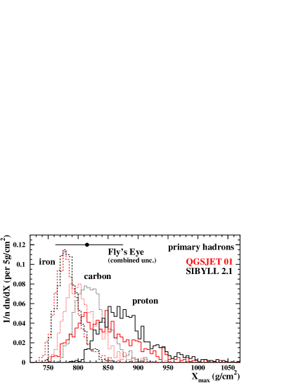
Figure 3: Shower maximum distributions of primary hadrons (iron $-$ dashed, carbon $-$ dotted, proton $-$ solid line), both for QGSJET 01 and SIBYLL 2.1. The measured value is indicated with the combined uncertainty, cf. Table 1.

The distributions of depth of shower maximum for various nuclear primaries and for the hadronic interaction models QGSJET 01 and SIBYLL 2.1 are shown in Figure 3. The reconstructed depth of the Fly’s Eye event of 815 g/cm² corresponds to a predicted average value of a mid-size nucleus. But due to the measurement uncertainties and due to the intrinsic shower fluctuations, any of the hadron primaries considered in both models could have produced the observed shower depth.

The average depth of shower maximum and its fluctuations are listed in Table 2. While the predictions for heavy nuclei agree for the two models, the difference for primary proton amounts to about 35 g/cm². Compared to SIBYLL 2.1, composition analyses based on QGSJET 01 would deduce somewhat lighter nuclei as primary particles using average shower maximum depths. However, for the current investigation this is of minor importance.

Table 2: Average depth and RMS of shower maximum for the given primary particle assumptions and discrepancy $\Delta$ to the observed shower maximum in units of standard deviations.

		QGSJET 01	SIBYLL 2.1
	photon	p     C     Fe	p     C     Fe
$X_{max}$ [g/cm2]	937	848   808   783	882   824   785
RMS($X_{max}$) [g/cm2]	26	54     30     22	47     27     19
$\Delta(X_{max})$ [$\sigma$]	1.9	0.6    0.4    0.6	0.9    0.4    0.6

Figure 4: Shower maximum distribution of primary photons compared to the reconstructed value of the Fly’s Eye event. The measured depth is shown with the combined uncertainty of $1\sigma_{c}$ and $2\sigma_{c}$, cf. Table 1.

In Figure 4, the $X_{max}$ distribution of primary photons is displayed. The Fly’s Eye event depth of maximum of 815 g/cm² is smaller than the average $X_{max}$ of primary photons of 937 g/cm². Given a combined uncertainty of 60 g/cm² for the measured $X_{max}$, the difference between these values is about two standard deviations.

To account also for shower fluctuations, the following method is applied to quantify the level of agreement between a primary particle hypothesis and the observation. For each profile $i$ with its individual shower maximum, the corresponding probability $P_{i}$ of consistency with data is determined. The total probability $P$ upon which the decision is based whether to reject a specific primary particle hypothesis is then calculated from all $n_{s}=1000$ profiles simulated per primary type as

$$P=\frac{1}{n_{s}}\sum_{i=1}^{n_{s}}P_{i}~{}.$$ (3)

In this approach, also possible non-Gaussian shower fluctuations predicted by the simulations are naturally taken into account. An incorrect consideration of shower fluctuations might introduce a significant bias in the primary type assignment, since the fluctuations are different for the various primary particles.

For primary photons, adopting the combined uncertainty of the data given in Table 1, a value of $P_{X_{max}}\simeq 6\%$ is obtained. This corresponds to a discrepancy of $\Delta\simeq 1.9\sigma$, where $\Delta$ is defined by $P(\chi^{2}\geq\Delta^{2})=6\%$ from the $\chi^{2}$ distribution for one degree of freedom. The discrepancy between data and calculation is listed in Table 2 for the different primary particle assumptions.

It might be instructive to illustrate the importance of reducing the measurement uncertainty. Assuming a resolution in $X_{max}$ of $\leq 30$ g/cm² as envisaged for the detectors of the Pierre Auger Observatory [33, 34], the discrepancy of primary photons to the reconstructed value would amount to $\geq 3.3\sigma$ instead of $1.9\sigma$.

3.2 Complete longitudinal profile

For the various hadron primaries, differences in the average number of particles (shower size) at maximum are known to be on the level of only a few percent and thus much smaller than the uncertainty in primary energy reconstruction of the Fly’s Eye event. In case of unconverted photons, the number of particles at maximum could be considerably reduced, which is accompanied by a change in the shape of the profile, as can be seen in Figure 2. For the specific conditions of the Fly’s Eye event, however, all simulated photons converted, and the differences in average shower size at maximum compared to primary hadrons are small ($<$8%). Also the profile shapes of the different primaries are in reasonable agreement to the data, as shown in Figure 5. Iron-initiated showers show slightly narrower profiles than, e.g., proton-induced ones. The difference is small, however, compared to the measurement uncertainties.

It seems worthwhile to mention that a quantity such as “number of particles” would require a precise definition if conclusions were attempted based on a direct comparison of shower sizes provided by different approaches. For instance, the number of tracked particles in Monte Carlo calculations depends on the simulation energy threshold [35]. Also, shower particles in three-dimensional calculations show an angular spread around the shower axis [36, 37], which should be kept in mind when comparing to an “effective” particle number in a one-dimensional calculation. However, due to the relatively large primary energy uncertainty of Fly’s Eye event, these items are of minor relevance for the present analysis.

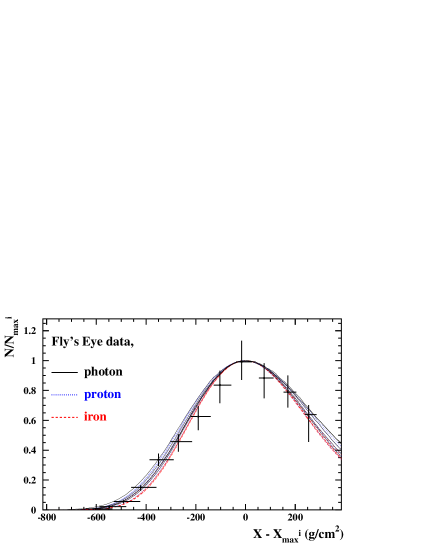
Figure 5: Profile shape of simulated showers initiated by photon, proton, and iron primaries (calculated with QGSJET 01) in comparison to the data. Each profile has been divided by the individual maximum number of particles $N_{max}^{i}$ and has been shifted by the respective depth of shower maximum $X_{max}^{i}$.

The complete longitudinal event profile is displayed together with simulated hadron-induced showers in Figure 6 and with photon-initiated events in Figure 7. Only a subset of the simulated events, picked at random, is plotted. The normalization of the calculated profiles has been chosen such that the number of particles at shower maximum roughly coincides with the reconstructed one of the Fly’s Eye event. More specifically, all CORSIKA shower size profiles are scaled by a factor 1.06 in case of primary photons and by 1.10 for primary hadrons, which is well within the reconstruction uncertainty of the primary energy.

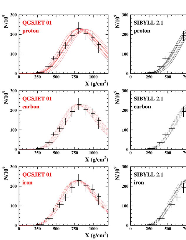
Figure 6: Typical longitudinal profiles of hadron-initiated showers compared to the data for different combinations of primary particle and hadronic interaction model as assigned.

Figure 7: Typical longitudinal profiles of photon-initiated showers compared to the data.

The profiles of the different hadron primaries show reasonable agreement with the data for both interaction models. In case of primary photons (Figure 7), differences between data and simulation are visible that can be attributed to a shift in atmospheric depth of the whole profile. Since the measured data points are constrained by a common geometry fit, it is important to note that their reconstructed atmospheric depth values are correlated [5]. Qualitatively, a shift in depth of each point by about 1.5 units of its standard deviation would results in a reasonable agreement of data and the photon profiles. In the following, a quantitative treatment for testing a primary particle assumption against the observed profile is described.

Shower fluctuations are taken into account as discussed in Section 3.1 by averaging the probabilities $P_{i}$ for the individual profiles to obtain an overall probability $P$ for each considered primary particle type (Eq. 3). The calculation of $P_{i}$ for each individual simulated profile is based on the reconstructed profile data as shown in Figure 7 assuming Gaussian probability density functions for the quoted uncertainties $dN_{j}$ and $dX_{j}$ of the data points. For the uncertainties $dX_{j}$, we take the point-to-point correlation into account and allow all data points to be shifted in the same direction by the same fraction $f\cdot dX_{j}$ when varying the reconstructed geometry. Given a simulated profile $i$, for a certain correlated shift of the $n_{d}=12$ data points in horizontal direction by $f_{k}\cdot dX_{j}$, a value $\chi^{2}_{ik}$ is then calculated as

$$\chi^{2}_{ik}=\sum_{j=1}^{n_{d}}\left(\frac{\Delta N_{jk}}{dN_{j}}\right)^{2}$$ (4)

with $\Delta N_{jk}=N_{j}-N_{sim}(X_{j}+f_{k}\cdot dX_{j})$ denoting the difference between the reconstructed event value $N_{j}$ and the simulated value $N_{sim}$ at depth $X_{j}+f_{k}\cdot dX_{j}$. Factors $f_{k}=-3.0,...,+3.0$ are adopted with a stepsize of $\Delta f=f_{k+1}-f_{k}=0.05$. From $\chi^{2}_{ik}$, the probability $P_{ik}$ that the $i$-th profile fits the shifted data is determined as

$$P_{ik}=P(\chi^{2}_{ik,{\rm gen}}\geq\chi^{2}_{ik})$$ (5)

by randomly generating a series of artificial data sets according to the uncertainties $dN_{j}$ around $N_{sim}(X_{j})$ and shifting each data set in the same way as the real data to obtain the distribution of $\chi^{2}_{ik,{\rm gen}}$ values [38]. The probability $P_{i}$ is then given by the sum

$$P_{i}=\sum_{k}w_{k}\cdot P_{ik}$$ (6)

where the individual $P_{ik}$ are weighted for step $k$ according to a Gaussian probability density function,

$$w_{k}=\frac{1}{\sqrt{2\pi}}~{}\int_{~{}~{}f_{k}-\frac{1}{2}\Delta f}^{f_{k}+\frac{1}{2}\Delta f}\exp(-z^{2}/2)~{}dz~{}~{}.$$ (7)

Figure 8: Distribution of probabilities $P_{i}$ for photon primaries, calculated as described in the text.

The resulting distribution of $P_{i}$ for the photon profiles is plotted in Figure 8. Most profiles reach values well above 5%. Following Eq. (3), an average probability $P\simeq 13\%$ is obtained. This corresponds to a discrepancy between photons and data of about 1.5$\sigma$. The results obtained for the primary photon and hadron hypotheses are summarized in Table 3.

Table 3: Probability $P$ of a given primary particle hypothesis to be consistent with the observed Fly’s Eye event profile and corresponding discrepancy $\Delta$ in units of standard deviations.

		QGSJET 01	SIBYLL 2.1
	photon	p     C     Fe	p     C     Fe
$P$ [%]	13	43    54    53	31    52    54
$\Delta$ [$\sigma$]	1.5	0.8   0.6   0.6	1.0   0.6   0.6

4 Discussion

For any considered primary hadron assumption and for both hadronic interaction models, the values given in Table 3 confirm that no hypothesis can be rejected, as expected from the $X_{max}$ investigation and in agreement with previous considerations in the literature [5, 6]. Also in the framework of the SIBYLL 2.1 model, primary protons, which on average reach the maximum $\simeq$70 g/cm² deeper in the atmosphere than the observed profile, are not excluded due to the measurement uncertainties and shower fluctuations. They are only slightly less favoured (discrepancy of 1.0$\sigma$ to data) with respect to heavier nuclei (0.6$\sigma$) or primary protons in the QGSJET 01 model (0.8$\sigma$).

Compared to primary hadrons, photons are less favoured. With a discrepancy to the Fly’s Eye event profile on the level of 1.5$\sigma$, however, also the primary photons are not excluded by the data.

This result does not confirm a previous analysis that claimed the primary photon hypothesis to be inconsistent with the experimental observations [6]. Compared to our calculations, the shower maximum of primary photons had been obtained at depths larger by $\simeq$90 g/cm². Part of this difference might arise from the preshower calculation, as might be expected due to the numerical error in Ref. [8] pointed out in Ref. [9]. Our analysis yields an average energy fraction carried by particles with energies above $10^{19}$ eV of $\simeq 40\%$ (compare Figure 1). As this is smaller than the value $>60\%$ given in [6], a “faster” shower development is expected, also due to the LPM effect being less important for smaller particle energies.

The discrepancy between photons and data might be diminished below 1.5$\sigma$ by additional uncertainties not yet considered in the quantitative treatment. For the simulated profiles, no “theoretical” uncertainty has been assumed when testing the primary photon hypothesis. Though much less affected by high-energy extrapolations of hadronic interactions than hadron primaries, uncertainties are associated, for instance, with the photonuclear cross-section at the highest energies. Given the specific conditions of the Fly’s Eye event, photonuclear reactions seem of minor importance. For photons around $10^{19}$ eV, the expected photonuclear cross-section [39] is more than two orders of magnitude below the pair production cross-section. As preshowering additionally distributes the initial primary energy among many particles entering the atmosphere, photonuclear interactions of a small subset of these particles (of order 1 out of 300 particles) impose only a marginal effect on the overall shower profile for the simulated primary photons. Allowing, however, for a larger increase of the photonuclear cross-section with energy, photon-initiated events would become more hadron-like. The expected photon profiles would be shifted towards the observed one which would reduce the discrepancy.

For the reconstructed data, recent studies of the atmospheric density profile [40] indicate a significant additional uncertainty in the reconstructed atmospheric depth. The air density profile is required for converting the altitude of a shower track observed by the telescope to its derived atmospheric depth, as the physics interpretation is mostly based on the latter quantity. Without proper correction, variations of the density profile might lead to misinterpretations of the reconstructed atmospheric depth of 10-20 g/cm² or more, depending on the specific conditions of the observation. Such density profile variations have been confirmed in investigations of atmospheric data taken at Salt Lake City airport, i.e. not far from the Fly’s Eye site, that are available starting from 1996 [41]. Moreover, a study of October density profiles measured over several years at Salt Lake City airport indicates a systematic underestimation of about 10$-$15 g/cm² on average in $X_{max}$ when using the US standard atmosphere for geometries similar to the Fly’s Eye event [42]. Assuming such a shift in atmospheric depth of the reconstructed profile, the discrepancy between photons and data would be reduced by $\simeq$0.2$\sigma$.

Even without assuming a re-analysis of the Fly’s Eye event that would push the data closer to the photons, it seems fair to conclude that additional uncertainties exist so that the potential to exclude a specific primary particle type hypothesis is reduced. This strengthens the conclusion that photons are not ruled out as primary particle for the Fly’s Eye event.

Clearly, a larger statistics of high-energy events is necessary to allow stringent constraints on the photon hypothesis. Let us illustrate the sensitivity of the Pierre Auger Observatory [33, 34] for giving an upper limit on the photon fraction in case no photon detection can be claimed. Depending on the actual high-energy particle flux and including a duty cycle of 10$-$15%, the fluorescence telescopes of the Auger experiment are expected to record about 30$-$50 shower profiles with primary energies exceeding $10^{20}$ eV within a few years of data taking. For simplicity, let us consider a constant probability $\epsilon$ for each of these $n$ observed profiles to be originated by a photon. Then, the probability that $n_{\gamma}$ out of $n$ profiles were photon-initiated is

$$P(n_{\gamma})=\epsilon^{n_{\gamma}}~{}(1-\epsilon)^{n-n_{\gamma}}~{}(^{~{}~{}n}_{n-n_{\gamma}})~{}~{}~{}.$$ (8)

For a choice of $n=40$ and $\epsilon=5\%$, with 95% confidence level a photon fraction exceeding 10% could be excluded, which would provide an important constraint for explaining the EHECR origin. In case of the Fly’s Eye event, a value of $\epsilon=5\%$ corresponds to reducing e.g. the uncertainties $dX_{j}$ by a factor 1.5, which seems well in reach for the Auger experiment. The sensitivity level from the profile measurements alone might even be increased, as the most energetic events will be observed from different telescope positions. Further improvement might be gained by including data from the Auger surface detectors. Apart from the virtually 100% duty cycle of this surface array, information on the muon content of the shower would additionally strongly constrain potential primary photons. The average muon number at observation level for the events simulated in the current analysis is given in Table 4. In case of photon primaries, the muon number is reduced by more than a factor 3 relative to hadron primaries. It is also interesting to note that the muon numbers predicted by QGSJET 01 and SIBYLL 2.1 differ quite significantly from each other. Compared to the overall profile, the muon number is much more sensitive to different extrapolations of hadronic interaction features to the highest energies. Combining the various observables will help to improve the modeling of hadron-initiated showers.

Table 4: Simulated average muon number and RMS on observation level for the Fly’s Eye event conditions.

		QGSJET 01	SIBYLL 2.1
	photon	p      C      Fe	p      C      Fe
$N_{\mu}/10^{8}$	3.1	12.9   14.0   15.3	9.6   11.0   11.8
RMS($N_{\mu}/10^{8}$)	0.3	1.5    0.8     0.6	1.2    0.6    0.5

Acknowledgements. We are grateful to Sergej Ostapchenko for drawing our attention to the profile analysis. We are indebted to Ralph Engel and Paul Sommers for comments on various aspects of the investigation. Very helpful discussions with Klaus Eitel on statistical methods and technical assistance from Dieter Heck for the simulations are kindly acknowledged. This work was partially supported by the Polish State Committee for Scientific Research under grants no. PBZ KBN 054/P03/2001 and 2P03B 11024 and by the International Bureau of the BMBF (Germany) under grant no. POL 99/013. MR is supported by the Alexander von Humboldt Foundation.

References

- [1] P. Bhattacharjee and G. Sigl, Phys.Rep. 327 (2000) 109
- [2] K. Shinozaki et al., ApJ 571 (2002) L117
- [3] M. Ave, J.A. Hinton, R.A. Vázquez, A.A. Watson, and E. Zas, Phys. Rev. D 65 (2002) 063007
- [4] R.M. Baltrusaitis et al., Nucl. Instr. Meth. A240 (1985) 410
- [5] D.J. Bird et al., ApJ 441 (1995) 144
- [6] F. Halzen, R.A. Vazquez, T. Stanev, and H.P. Vankov, Astropart. Phys. 3 (1995) 151
- [7] S. Karakula and W. Bednarek, Proc. Int. Cosmic Ray Conf., Rome (1995) 266
- [8] T. Erber, Rev. Mod. Phys. 38 (1966) 626
- [9] P. Homola, D. Góra, D. Heck, H. Klages, J. Pȩkala, M. Risse, B. Wilczyńska, and H. Wilczyński, Simulation of Ultra-High Energy Photon Propagation in the Geomagnetic Field, submitted to Comput. Phys. Commun. (2003); preprint astro-ph/0311442
- [10] A.A. Watson, Ultrahigh Energy Cosmic Rays: The Present Position and the Need for Mass Composition Measurements, Invited talk at Conference on Thinking, Observing and Mining the Universe, Sorrento, Italy (2003); preprint astro-ph/0312475
- [11] D. Heck, J. Knapp, J.N. Capdevielle, G. Schatz, and T. Thouw, Report FZKA 6019, Forschungszentrum Karlsruhe (1998); www-ik.fzk.de/~heck/corsika
- [12] N.N. Kalmykov, S.S. Ostapchenko, and A.I. Pavlov, Nucl. Phys. B (Proc. Suppl.) 52B (1997) 17; D. Heck et al., Proc. Int. Cosmic Ray Conf., Hamburg 1 (2001) 233
- [13] R. Engel, T.K. Gaisser, P. Lipari, and T. Stanev, Proc. Int. Cosmic Ray Conf., Salt Lake City 1 415 (1999); R.S. Fletcher, T.K. Gaisser, P. Lipari, and T. Stanev, Phys. Rev. D 50 5710 (1994); J. Engel, T.K. Gaisser, P. Lipari, and T. Stanev, Phys. Rev. D 46 (1992) 5013
- [14] J.W. Elbert and P. Sommers, ApJ 441 (1995) 151
- [15] A.A. Sokolov and I.M. Ternov, Radiation from Relativistic Electrons, Springer, Berlin (1986)
- [16] B. McBreen and C.J. Lambert, Phys. Rev. D 24, (1981) 2536
- [17] F.A. Aharonian, B.L. Kanewsky, and V.V. Vardanian, Astrophys. Space Sci. 167 (1990) 111
- [18] H.P. Vankov and P. Stavrev, Phys. Lett. B 266 (1991) 178
- [19] T. Stanev and H.P. Vankov, Phys. Rev. D 55 (1997) 1365
- [20] X. Bertou, P. Billoir, and S. Dagoret-Campagne, Astropart. Phys. 14 (2000) 121
- [21] A.V. Plyasheshnikov and F.A. Aharonian, J. Phys. G 238 (2002) 267
- [22] W. Bednarek, New Astron. 7 (2002) 471
- [23] H.P. Vankov, N. Inoue, and K. Shinozaki, Phys. Rev. D 67 (2003) 043002
- [24] National Geophysical Data Center, USA, www.ngdc.noaa.gov
- [25] W.R. Nelson, H. Hirayama, and D.W.O. Rogers, Report SLAC 265, Stanford Linear Accelerator Center (1985)
- [26] L.D. Landau and I.Ya. Pomeranchuk, Dokl. Akad. Nauk SSSR 92 (1953) 535 & 735 (in Russian); A.B. Migdal, Phys. Rev. 103 (1956) 1811
- [27] D. Heck and J. Knapp, Report FZKA 6097, Forschungszentrum Karlsruhe (1998), available from www-ik.fzk.de/~heck/publications. An error in the implementation of the LPM effect in CORSIKA was corrected in 2003 with the help of H.P. Vankov (R. Engel and D. Heck (2003), private communication). Depths of shower maximum obtained for unconverted photons with the corrected CORSIKA version 6.16 [9] that is used in the present analysis are in reasonable agreement to values given in [23] obtained with the AIRES code [28].
- [28] S.J. Sciutto, preprint astro-ph/9911331 (1999)
- [29] A.M. Hillas, Nucl. Phys. B (Proc. Suppl.) 52B (1997) 29
- [30] M. Kobal, Pierre Auger Collaboration, Astropart. Phys. 15 (2001) 259
- [31] M. Risse, D. Heck, J. Knapp, and S.S. Ostapchenko, Proc. Int. Cosmic Ray Conf., Hamburg 2 (2001) 522
- [32] M. Risse and D. Heck, Auger Internal Note GAP-2002-043, www.auger.org, (2002)
- [33] Auger Collaboration, The Pierre Auger Observatory Design Report (2nd ed.), Fermilab, Batavia Ill. (1997), www.auger.org/admin/DesignReport
- [34] J. Abraham et al., Auger Collaboration, accepted by Nucl. Inst. Meth. (2003); J. Blümer for the Auger Collaboration, J. Phys. G: Nucl. Part. Phys. 29 (2003) 867
- [35] F. Nerling, R. Engel, C. Guérard, L. Perrone, and M. Risse, Proc. Int. Cosmic Ray Conf., Tsukuba (2003)
- [36] J. Alvarez-Muñiz, E. Marqués, R.A. Vázquez, and E. Zas, Phys. Rev. D 67 (2003) 101303
- [37] M. Risse and D. Heck, Astropart. Phys. 20 (2004) 661; preprint astro-ph/0308158
- [38] L. Lyons, Statistics for nuclear and particle physicists, Cambridge University Press (1986)
- [39] M.M. Block, E.M. Gregores, F. Halzen, and G. Pancheri, Phys. Rev. D 60 (1999) 054024; M.M. Block, F. Halzen, and G. Pancheri, Eur. Phys. J. C 23 (2002) 329
- [40] B. Keilhauer, J. Blümer, H. Klages, and M. Risse, Proc. Int. Cosmic Ray Conf., Tsukuba (2003) 879; B. Keilhauer et al., publication in preparation
- [41] B. Wilczyńska, D. Góra, P. Homola, B. Keilhauer, H. Klages, J. Pȩkala, and H. Wilczyński, Proc. Int. Cosmic Ray Conf., Tsukuba (2003) 571
- [42] B. Wilczyńska et al., publication in preparation