Anisotropies in Ultrahigh Energy Cosmic Rays

Abstract

The present status of anisotropy studies for the highest energy cosmic rays is presented including the first full sky survey. Directions and prospects for the future are also discussed in light of new statistical methods and the last quantities of data expected in the near future from the Pierre Auger Observatory.

1 Introduction

Ultrahigh energy cosmic rays (UHECR’s) are among the most enigmatic phenomena in the universe.[1] In the mid-60’s Greisen, Zatsepin, and Kuzmin (GZK) pointed out that ultra high energy protons interact with the all-pervading cosmic microwave background via photopion production.[2] Strictly speaking, protons with energies $>10^{19.6}$ eV have a mean interaction length $<6$ Mpc and an inelasticity of about $20\%$ per interaction. Consequently, the popular astronomical picture, namely proton “bottom-up” acceleration in extragalactic objects, predicts a sharp suppression of the cosmic ray intensity somewhat beyond $10^{19.8}$ eV. For heavy nuclei, the giant dipole resonance can be excited at similar total energies and hence iron nuclei do not survive fragmentation over comparable path lengths.[3]

The existence of cosmic rays with energies exceeding $10^{20}$ eV has been observed by the Volcano Ranch,[4] the Haverah Park,[5] the Sydney University Giant Airshower Recorder (SUGAR),[6] the Akeno Giant Air Shower Array (AGASA),[7] and the Fly’s Eye[8] experiments. Because of the GZK cutoff, these cosmic rays should be produced in nearby active astronomical objects. Such high energy “stars” have been searched for in the arrival direction of these events but no clear candidates were found.

Of course, there are ways to avoid the distance restriction imposed by the GZK effect. For instance, there could be a “top-down” mechanism where (charged and/or neutral) supermassive $X$-particles are produced at extreme energies. Sources of these exotic particles could be topological defects left over from early universe phase transitions associated with the spontaneous symmetry breaking that underlies unified models of high energy interactions,[9] or else some long-lived metastable super-heavy relic particles produced through vacuum fluctuations during the inflationary stage of the universe.[10] From time to time, the energy stored in a single $X$ can be released in the form of massive quanta that typically produce jets of hadrons well above the highest observed energies. However, it is noteworthy that there can be a problem with some top-down interpretations. Specifically, the $X$-particle cascades may produce a rather large flux of energetic photons and neutrinos, possibly in excess of the upper limits already established.[11] The lack of plausible nearby astrophysical sources has also encouraged the idea of positing undiscovered neutral hadrons,[12] as well as mechanisms which are able to break the GZK barrier.[13] Even though sufficiently heavy particles would avoid photopion production (the threshold energy varies as the square of the mass of the first resonant state), the existence of these particles now appears to be excluded by laboratory experiments.[14] The only standard model particle that can reach our galaxy from high redshift sources without significance loss of energy is the neutrino. However, the expected event rate for early development of a neutrino shower is less than that of an electromagnetic or hadronic interaction by several orders of magnitude, even if ones takes into account non-standard graviton mediated interactions.[15]

The distribution of arrival directions is perhaps the most helpful observable in yielding clues about cosmic ray origin. This may come either from clustering on a small angular scale that identifies discrete sources,[16] or else as a large-scale celestial pattern that characterizes a particular class of potential sources.[17] Along these lines, data observed by the AGASA,[18] the SUGAR,[19] and the Fly’s Eye [20] experiments show an excess flux of cosmic rays from a direction near the Galactic center up to about $10^{18.5}$ eV, but there is evidence for Galactic plane avoidance above that energy. Such an effect can be easily explained if cosmic rays are mostly protons and nuclei, because their magnetic rigidity increases with energy and so one expects the angular width of the Galactic plane as seen in protons and nuclei would shrink slowly with rising energy. Moreover, the events yielding the observed anisotropy are concentrated in a limited energy range. This is very suggestive of neutrons as candidate primaries, because the directional signal requires relatively-stable neutral primaries, and time-dilated neutrons can reach Earth from typical Galactic distances when the neutron energy exceeds $10^{18}$ eV. Arguably, if the Galactic messengers are neutrons, then those with energies below $10^{18}$ eV will decay in flight, providing a flux of cosmic antineutrinos above a TeV which is observable at a kilometer-scale neutrino observatory.[21] A measurement of this flux can serve to identify the first extraterrestrial point source of TeV antineutrinos.

All in all, the data around $10^{18.5}$ eV suggests that a new population of cosmic rays with extragalactic origin begins to dominate the more steeply falling Galactic population. In the extragalactic sway, the evidence for anisotropy patterns is suggestive but statistically very weak. On the one hand, correlations with the local structure of galaxies have been reported,[22] suggesting that all cosmic rays with energies $>10^{18.5}$ eV are emitted by nearby astrophysical sources. On the other hand, possible correlations with high redshift astrophysical objects, which most likely indicate new physics, are also under debate.[23] Clearly, a positive identification of ultra high energy cosmic ray sources from the distribution of arrival directions requires a careful study of such distribution over the full celestial sphere. The latter is the main inspiration for this talk, which is organized as follows. In order to set the stage for the full-sky coverage discussion, in Sec. 2 I will present an overview of available statistics and existing anisotropy studies. In particular, I will concentrate on the SUGAR and AGASA experiments and discuss in some detail the exposure of these ground arrays. Next, in Sec. 3, I will review the main properties of the angular power spectrum[24] and study cosmic ray anisotropies from an expansion on spherical harmonics for modes out to $\ell=5$.[25] In Sec. 4 a numerical likelihood approach to the determination of cosmic ray anisotropies is presented.[26] This method offers many advantages over other approaches: It allows a wide range of statistically meaningful hypotheses to be compared even when full sky coverage is unavailable, can be readily extended in order to include measurement errors, and makes maximum unbiased use of all available information. Finally, I will summarize and present the conclusions in Section 6.

2 Experimental data sets

The SUGAR array was operated from January 1968 to February 1979 in New South Wales (Australia) at a latitude of $30.5^{\circ}$ South and longitude $149^{\circ}38^{\prime}$ East.[27] The array consisted of 47 independent stations on a rectangular grid covering an area $S\approx 70$ km². The primary energy was determined from the total number of muons, $N_{\mu}$, traversing the detector at the measured zenith angle $\theta$. The total aperture for incident zenith angles between $\theta_{1}$ and $\theta_{2}$ was found to be

$$A=\int_{\theta_{1}}^{\theta_{2}}S\,\,p(N_{\mu},\theta)\,\cos\theta\,d\Omega\,.$$ (1)

Here, $p(N_{\mu},\theta)$ is the probability that a shower falling within the physical area was detected, $S\cos\theta$ is the projected surface of the array in the shower plane, and $d\Omega$ is the acceptance solid angle. The SUGAR Collaboration reports[27] a reasonable accuracy in assessing the shower parameters up to $\theta=73^{\circ}$. The estimated angular uncertainty for showers that triggered 5 or more stations is reported as $3^{\circ}\sec\theta$.[27] However, the majority of events were only viewed by 3 or 4 stations, and for these the resolution appears to be as poor as $10^{\circ}$.[28] Of particular interest for this analysis, $p(N_{\mu}>10^{8},\theta<55^{\circ})\approx 0.85$,[29] yielding a total aperture $A\approx 125$ km² sr. This provides an exposure reasonably matched to that of AGASA, which is described next.

The AGASA experiment occupies farm land near the village of Akeno (Japan) at a longitude of $138^{\circ}30^{\prime}$ East and latitude $35^{\circ}30^{\prime}$ North.[30] The array, which consists of 111 surface detectors deployed over an area of about 100 km², has been running since 1990. About 95% of the surface detectors were operational from March to December 1991, and the array has been fully operational since then. A prototype detector operated from 1984 to 1990 and has been part of AGASA since 1990.[31] The aperture for events with primary zenith angle $0^{\circ}<\theta<45^{\circ}$ and energies beyond $10^{19.25}$ eV is found to be $A\approx 125$ km² sr.[30] The angular resolution for these events is $1.6^{\circ}$.[32]

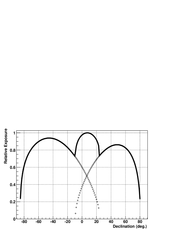
Figure 1: Declination dependence of SUGAR and AGASA relative apertures (dotted). The solid line indicates the combined relative aperture.

A detector at latitude $a_{0}$ that has continuous operation with constant exposure in right ascension and is fully efficient for $\theta<\theta_{\rm max}$ has relative exposure with the following dependence on declination[33]

$$\omega(\delta)\propto(\cos a_{0}\,\,\cos\delta\,\,\sin\alpha_{\rm max}+\alpha_{\rm max}\,\,\sin a_{0}\,\,\sin\delta)\,\,,$$ (2)

where $\alpha_{\rm max}$, the local hour angle at which the zenith angle becomes equal to $\theta_{\rm max}$, is given by

$$\alpha_{\rm max}=\left\{\begin{array}[]{ll}0&{\rm if}\,\,\,\xi>1\\ \pi&{\rm if}\,\,\,\xi<-1\\ \cos^{-1}\,\,\xi&{\rm otherwise}\end{array}\right.$$ (3)

with

$$\xi\equiv\frac{\cos\theta_{\rm max}-\sin a_{0}\,\,\sin\delta}{\cos a_{0}\,\,\,\cos\delta}\,\,.$$ (4)

The resulting declination dependence for SUGAR and AGASA together with the combined aperture is given in Fig. 1.

As one can readily see in Fig. 1, the combined aperture of SUGAR and AGASA arrays is nearly uniform over the entire sky. The expected event rate is found to be

$$\frac{dN}{dt} = A\,\int_{E_{1}}^{E_{2}}\,E^{3}J(E)\,\frac{dE}{E^{3}}$$ (5)

$$\approx \frac{A}{2}\,\langle E^{3}\,J(E)\rangle\,\left[\frac{1}{E_{1}^{2}}-\frac{1}{E_{2}^{2}}\right]\,\,,$$

where $\langle E^{3}J(E)\rangle\approx 10^{24.6}$ eV² m^-2 s^-1 sr^-1 stands for the observed ultra high energy cosmic ray flux, which has a cutoff at $E_{2}=10^{20.5}$ eV.[1] Thus, in approximately 10 yr of running each of these experiments should collect $\approx 50$ events above $E_{1}=10^{19.6}$ eV, arriving with a zenith angle $<\theta_{\rm max}$. Here, $\theta_{\rm max}=45^{\circ}$ for AGASA and $\theta_{\rm max}=55^{\circ}$ for SUGAR. Our sub-sample for the full-sky anisotropy search consists of the 50 events detected by AGASA from May 1990 to May 2000,[34] and the 49 events detected by SUGAR with $\theta<55^{\circ}$.[27] Note that we consider the full data sample for the 11 yr lifetime of SUGAR (in contrast to the 10 yr data sample from AGASA). This roughly compensates for the time variation of the sensitive area of the experiment as detectors were deployed or inactivated for maintenance. The arrival directions of the 99 events are plotted in Fig. 2 (equatorial coordinates B.1950).

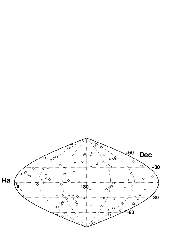
Figure 2: Arrival direction of the 99 events observed above $10^{19.6}$ eV by the SUGAR ($\theta<55^{\circ}$) and the AGASA ($\theta<45^{\circ}$) experiments (equatorial coordinates B.1950).

3 Correlations and Power Spectrum

We begin this section with a general introduction to the calculation of the angular power spectrum and the determination of the expected size of intensity fluctuations. The technique is then applied to the AGASA and SUGAR data in order to check for fluctuations beyond those expected from an isotropic distribution.

Let us start by defining the directional phase space of the angular distribution of cosmic ray events in equatorial coordinates, $(\alpha,\delta)$. (i) The direction of the event is described by a unit vector

$${\bf n}=\sin\delta\,({\bf i}\,\cos\alpha+{\bf j}\,\sin\alpha)+{\bf k}\,\cos\delta\,\,;$$ (6)

(ii) The solid angle is given by

$$d^{2}{\bf n}=\sin\delta\,\,d\delta\,d\alpha\,\,;$$ (7)

(iii) The delta function for the solid angle is defined as

$$\delta({\bf n},{\bf n}^{\prime})=\delta(\cos\delta-\cos\delta^{\prime})\,\sum_{m=-\infty}^{\infty}\delta(\alpha-\alpha^{\prime}+2\pi m)\,,$$ (8)

so that, as usual,

$$f({\bf n})=\int\delta({\bf n},{\bf n}^{\prime})\,\,f({\bf n}^{\prime})\,\,d^{2}{\bf n}^{\prime}\,\,;$$ (9)

(iv) The probability distribution $P({\bf n})d^{2}{\bf n}$ of events can be employed for the purpose of computing the averages

$$\overline{f}=\int f({\bf n})\,\,P({\bf n})\,\,d^{2}{\bf n}\,\,;$$ (10)

Finally, (v) for a sequence of $N$ different cosmic ray events $({\bf n}_{1},\ldots,{\bf n}_{N})$ one may assume an independent distributions for each event, i.e.

$$P_{N}({\bf n}_{1},\ldots,{\bf n}_{N})\prod_{i}^{N}d^{2}{\bf n}_{i}=\prod_{i}^{N}\{P({\bf n}_{i})\,d^{2}{\bf n}_{i}\}\,\,.$$ (11)

For a sequence of events $({\bf n}_{1},\ldots,{\bf n}_{N})$ let us describe the angular intensity as the random variable

$$I({\bf n})=\frac{1}{N}\sum_{j=1}^{N}\,\delta({\bf n},{\bf n}_{j})\,\,.$$ (12)

From Eqs. (11) and (12) it follows that

$$\overline{I({\bf n})} = \int\ldots\int I({\bf n})\,P_{N}({\bf n}_{1},\ldots,{\bf n}_{N})\,\prod_{i}^{N}d^{2}{\bf n}_{i}$$ (13)

$$= P({\bf n}).$$

The two point correlation function $G({\bf n},{\bf n}^{\prime})=\overline{I({\bf n})I({\bf n}^{\prime})}$ is defined via

$$G({\bf n},{\bf n}^{\prime}) = \int\ldots\int I({\bf n})\ I({\bf n}^{\prime})\ P_{N}({\bf n}_{1},\ldots,{\bf n}_{N})\ \prod_{i}^{N}d^{2}{\bf n}_{i}$$

$$= \frac{1}{N}\,\delta({\bf n},{\bf n}^{\prime})\,P({\bf n})+\left(1-\frac{1}{N}\right)\,P({\bf n})\,P({\bf n}^{\prime})\,\,.$$

The “power spectrum” of the correlation function is determined by the eigenvalue equation

$$\int G({\bf n},{\bf n}^{\prime})\,\,\psi_{\lambda}({\bf n}^{\prime})\,\,d^{2}{\bf n}^{\prime}=\lambda\,\,\psi_{\lambda}({\bf n}).$$ (15)

In this regard it is useful to introduce Dirac notation to indicate the inner product

$$\left<\psi|\psi\right>=\int\psi^{*}({\bf n})\,\,\psi({\bf n})\,\,d^{2}{\bf n}\,\,.$$ (16)

With this in mind, Eq. (15) reads

$$G\,\left|\psi_{\lambda}\right>=\lambda\,\left|\psi_{\lambda}\right>.$$ (17)

In the limit of a large number of events $N\to\infty$,

$$\lim_{N\to\infty}G({\bf n},{\bf n}^{\prime})\equiv G_{\infty}({\bf n},{\bf n}^{\prime})=P({\bf n})P({\bf n}^{\prime})\,,$$ (18)

or equivalently,

$$\hat{G}_{\infty}=\left|P\right>\left<P\right|\,.$$ (19)

In such a limit, fluctuations can be neglected and we find only two possible values in the spectrum: (i) There is a non-degenerate non-zero eigenvalue

$$\hat{G}_{\infty}\left|P\right>=\lambda_{\infty}\left|P\right>\,,$$ (20)

with

$$\lambda_{\infty}=\left<P|P\right>=\int P^{2}({\bf n})d^{2}{\bf n}.$$ (21)

(ii) For every state $\left|f\right>$ orthogonal to $\left|P\right>$ with mean value $\bar{f}=\left<P|f\right>=0$, there exists a zero eigenvalue in the power spectrum

$$\hat{G}_{\infty}\left|f\right>=\left|P\right>\left<P|f\right>=\left\{\int Pfd^{2}{\bf n}\right\}\left|P\right>=\bar{f}\left|P\right>=0\,\,.$$ (22)

Let us now turn to consider the effects of finite $N$. Defining the fluctuations in the intensity by

$$\Delta I({\bf n})=I({\bf n})-\overline{I({\bf n})}=I({\bf n})-P({\bf n}),$$ (23)

the two point correlation function can be re-written as

$$G({\bf n},{\bf n}^{\prime}) = \overline{I({\bf n})I({\bf n}^{\prime})}=\overline{I({\bf n})}\ \overline{I({\bf n}^{\prime})}+\overline{\Delta I({\bf n})\Delta I({\bf n}^{\prime})}$$ (24)

$$= G_{\infty}({\bf n},{\bf n}^{\prime})+\overline{\Delta I({\bf n})\Delta I({\bf n}^{\prime})}\,,$$

with

$$\overline{\Delta I({\bf n})\Delta I({\bf n}^{\prime})}=\frac{1}{N}\,\left[\,\delta({\bf n},{\bf n}^{\prime})P({\bf n})-P({\bf n})P({\bf n}^{\prime})\,\right]\,,$$ (25)

where Eq. (LABEL:CP8) has been invoked. Putting all this together, some general results follow: (i) For the $N\to\infty$ case, there is only one state with a finite eigenvalue $\lambda_{\infty}$, while the rest of the power spectrum corresponds to $\lambda=0$. (ii) For finite $N$, Eq. (25) implies that the fluctuations are of order $N^{-1}$. The power spectrum for large $N$ then has one eigenvalue of order unity and the rest of the eigenvalues are of order $N^{-1}$.

Now, for an isotropic distribution of ${\bf n}$,

$$\widetilde{P}({\bf n})=\frac{1}{4\pi}\,\,,$$ (26)

and the two point correlation function reads,

$$\widetilde{G}({\bf n},{\bf n}^{\prime})=\frac{1}{4\pi N}\,\,\delta({\bf n},{\bf n}^{\prime})+\frac{1}{(4\pi)^{2}}\,\left({1-\frac{1}{N}}\right)\,\,.$$ (27)

The eigenvalue problem is solved by employing spherical harmonics [35]

$$\int\widetilde{G}({\bf n},{\bf n}^{\prime})\,\,Y_{lm}({\bf n}^{\prime})\,d^{2}{\bf n}^{\prime}=\lambda_{\ell m}\,\,Y_{\ell m}({\bf n})\,\,,$$ (28)

where

$$\lambda_{\ell m}=\left\{\begin{array}[]{ll}(4\pi)^{-1}&\hskip 28.45274pt\textrm{if $(\ell,m)=(0,0)$}\\ (4\pi N)^{-1}&\hskip 28.45274pt\textrm{if $(\ell,m)\neq(0,0)$}\end{array}\right.\,.$$ (29)

The eigenfunctions form a useful set for expansions of the intensity over the celestial sphere

$$I({\bf n})=\sum_{\ell=0}^{\infty}\,\,\sum_{m=-\ell}^{\ell}\,\,a_{\ell m}\,Y_{\ell m}({\bf n})\,\,.$$ (30)

To incorporate the dependence on declination given in Eq. (2), let us re-define the angular intensity

$$I({\bf{n}})=\frac{1}{\mathcal{N}}\,\,\sum_{j=1}^{N}\frac{1}{\omega_{j}}\,\,\delta({\bf n},{\bf n}_{j})\,\,,$$ (31)

where $\omega_{j}$ is the relative exposure at arrival direction ${\bf n}_{j}$ and ${\mathcal{N}}$ is the sum of the weights $\omega_{j}^{-1}$. Since the eigenvalues of the $Y_{\ell m}$ expansion are uniquely defined

$$a_{\ell m}=\int I({\bf n})\,\,Y_{\ell m}({\bf n})\,\,d^{2}{\bf n}\,\,,$$ (32)

the replacement of Eq. (31) into Eq. (32) leads to the explicit form of the coefficients for our set of arrival directions

$$a_{\ell m}=\frac{1}{{\mathcal{N}}}\sum_{j=1}^{N}\,\frac{1}{\omega_{j}}\,\,Y_{\ell m}({\bf n}_{j})\,.$$ (33)

With the coeffients given in this way, one can plot the intensity of the cosmic ray sky using Eq. 30, as seen in Fig. 3.

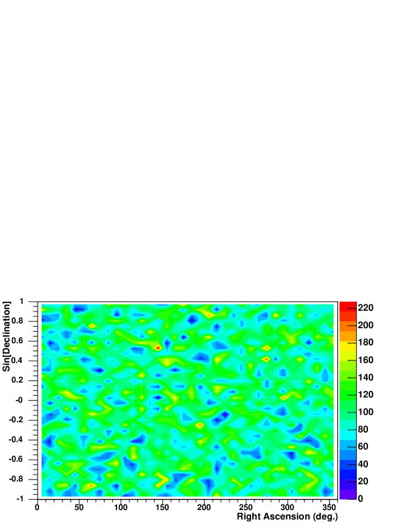
Figure 3: Intensity of the cosmic ray sky in equatorial coordinates as seen by the SUGAR and AGASA arrays.

The mean square fluctuations of the coefficients are determined by the power spectrum eigenvalues according to

$$\overline{a_{\ell m}^{2}}=\lambda_{\ell m}.$$ (34)

Although full anisotropy information is encoded into the coefficients $a_{\ell m}$ (tied to some specified coordinate system), the (coordinate independent) total power spectrum of fluctuations

$$C(\ell)=\frac{1}{(2\ell+1)}\,\,\sum_{m=-\ell}^{\ell}a_{\ell m}^{2}\,\,,$$ (35)

provides a gross summary of the features present in the celestial distribution together with the characteristic angular scale(s). Note that Eqs. (29) and (34) imply

$$\overline{C}(\ell)=\frac{1}{(2\ell+1)}\,\,\sum_{m=-\ell}^{\ell}\overline{a_{\ell m}^{2}}\,=\left\{\begin{array}[]{ll}(4\pi)^{-1}&\textrm{if $\ell=0$}\\ (4\pi N)^{-1}&\textrm{if $\ell\neq 0$}\end{array}\right.\,.$$ (36)

The power in mode $\ell$ is sensitive to variation over angular scales of $\ell^{-1}$ radians.[33] Recalling that the estimated angular uncertainty for some of the events in the SUGAR sample is possibly as poor as $10^{\circ}$ [28] we only look in this study for large scale patterns, going into the multipole expansion out to $\ell=5$.

Our results at this juncture are summarized in Fig. 4. The angular power spectrum is consistent with that expected from a random distribution for all (analyzed) multipoles, though there is a small ($2\sigma$) excess in the data for $\ell=3$. The majority of this excess comes from SUGAR data.[36] The decrease in error as $\ell$ increases may be understood as a consequence of the fact that contributions to mode $\ell$ arise from variations over an angular scale $\ell^{-1}$. If one compares to the expectation for isotropy, structures characterized by a smaller angular scale, and hence larger $\ell$, can be ruled out with more significance than larger structures.

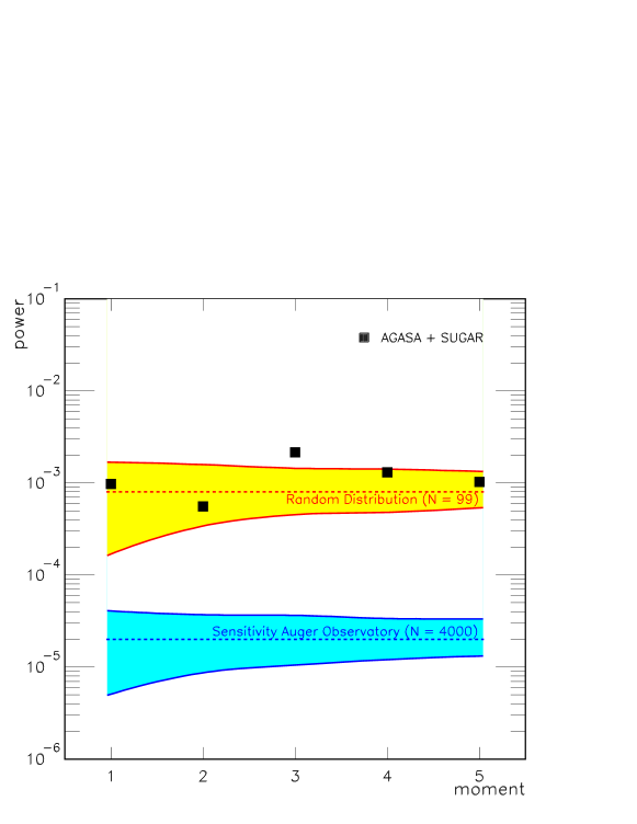
Figure 4: The angular power spectrum is indicated by the squares. The horizontal lines indicate the mean value, $\overline{C}(\ell)=(4\pi N)^{-1},$ expected for an isotropic distribution. The upper shaded band shows the 1$\sigma$ fluctuation around the mean value for $N=99$. The band was obtained from 1000 sets of Monte Carlo simulations of 99 events each, including small corrections for $\omega_{i}$. For $\ell=3$, where there is a small excess compared to the expectation for isotropy, $C(3)=2.16\times 10^{-3}$ while the expectation from a random distribution is $\overline{C}_{\rm MC}(3)=9.5\times 10^{-4}$, with a variance of $5.0\times 10^{-4}$. The projected sensitivity for the Pierre Auger Observatory is also indicated on the plot by the lower shaded band.

To quantify the error, we study the fluctuations in $C(\ell)$ for $\ell\geq 1$. For simplicity, let us neglect the small effects of declination (viz., $\omega_{i}=1\,\,\forall i$), and consider the random variable

$$X_{\ell}=\frac{C(\ell)}{\overline{C}(\ell)}=\left(\frac{4\pi N}{2\ell+1}\right)\sum_{m=-\ell}^{\ell}a_{\ell m}^{2}.$$ (37)

Denoting by $P_{\ell}(\cos\delta)$ the Legendre polynomial of order $\ell$ and employing the addition theorem for spherical harmonics,

$$\frac{4\pi}{2\ell+1}\sum_{m=-\ell}^{\ell}Y_{\ell m}({\bf n})Y_{\ell m}({\bf n}^{\prime})=P_{\ell}({\bf n\cdot n}^{\prime})\,,$$ (38)

Eqs. (33), (37), and (38) imply that

$$X_{\ell}=1+\frac{2}{N}\sum_{1\leq i<j\leq N}P_{\ell}({\bf n}_{i}\cdot{\bf n}_{j}).$$ (39)

Evidently, $\overline{X_{\ell}}=1$. Besides,

$$\overline{X_{\ell}^{2}}=1+\frac{4}{N^{2}}\sum_{1\leq i<j\leq N}\ \sum_{1\leq k<q\leq N}\overline{P_{\ell}({\bf n}_{i}\cdot{\bf n}_{j})P_{\ell}({\bf n}_{k}\cdot{\bf n}_{q})}\,.$$ (40)

Since different pairs in the sum on the right hand side of Eq. (40) are uncorrelated, it follows that

$$\overline{X_{\ell}^{2}}=1+\frac{4}{N^{2}}\sum_{1\leq i<j\leq N}\overline{P_{\ell}({\bf n}_{i}\cdot{\bf n}_{j})^{2}}\,.$$ (41)

There are $\{N(N-1)/2\}$ equivalent pairs in Eq. (41) which implies

$$\overline{X_{\ell}^{2}}=\overline{X_{\ell}}^{2}+2\left(1-\frac{1}{N}\right)\overline{P_{\ell}({\bf n}_{1}\cdot{\bf n}_{2})^{2}}\,.$$ (42)

From Eq. (38) we obtain

$$\overline{P_{\ell}({\bf n}_{1}\cdot{\bf n}_{2})^{2}} = \left(\frac{4\pi}{2\ell+1}\right)^{2}\sum_{m=-l}^{l}\overline{Y_{\ell m}({\bf n}_{1})^{2}}\ \overline{Y_{\ell m}({\bf n}_{2})^{2}}$$ (43)

$$= \frac{1}{2\ell+1}\,.$$

Plugging Eq. (43) into Eq. (42) leads to

$$\overline{\Delta X_{\ell}^{2}}=\left(1-\frac{1}{N}\right)\frac{2}{2\ell+1},$$ (44)

or equivalently,

$$\left(\frac{\overline{\Delta C_{\ell}}^{2}}{\overline{C_{\ell}}^{2}}\right)=\left(1-\frac{1}{N}\right)\frac{2}{2\ell+1}\,,$$ (45)

yielding (for large $N$)

$$\lim_{N\to\infty}\left(\frac{\overline{\Delta C_{\ell}}^{2}}{\overline{C_{\ell}}^{2}}\right)=\frac{2}{2\ell+1}\ \ {\rm for}\ \ \ell\geq 1\,,$$ (46)

which is the variance on $X_{\ell}$.

4 Numerical Likelihood Analysis of Cosmic Ray Anisotropies

The approach described above requires what might be described as “reasonably good statistics”. That is to say, one needs to have essentially some reasonable acceptance for every element of solid angle in the sky. Problems of interpretation can easily arise if there are regions which are unobservable – blind spots – and in this section I briefly describe how these can be dealt with numerically. The work follows closely that presented in [40].

4.1 Spherical Harmonics

It is convenient to define a set of real spherical harmonics $\{\psi_{\ell,m}\}$ for $\ell=0,1,2,\ldots$ and $m=-\ell,-(\ell-1),\ldots,0,\dots,(\ell-1),\ell$ by

$$\psi_{\ell,m}(\theta,\phi)=\left\{\begin{array}[]{ll}k_{\ell}^{|m|}P_{\ell}^{|m|}(\cos\theta)\cos(m\phi)&\mbox{for\ $m=-\ell,\ldots,-1$},\\ k_{\ell}^{0}P_{n}^{0}(\cos\theta)&\mbox{for\ $m=0$,}\\ k_{\ell}^{m}P_{\ell}^{m}(\cos\theta)\sin(m\phi)&\mbox{for\ $m=1,\ldots,\ell$}\end{array}\right.$$ (47)

which are orthonormal with respect to the usual measure $\sin(\theta)d\theta d\phi$ and integration over $\theta$ from 0 to $\pi$ and $\phi$ from 0 to $2\pi$, the $P_{\ell}^{m}$ are associated Legendre polynomials of the first kind, and the normalization constants $k^{\ell}_{m}$ are:

$$k_{0}^{0}=\frac{1}{\sqrt{2\pi}},k_{\ell}^{0}=\sqrt{\frac{2\ell+1}{4\pi}},{\mathrm{\ and\ }}k_{\ell}^{m}=\sqrt{\frac{2\ell+1}{2\pi}\frac{(\ell-m)!}{(\ell+m)!}}$$ (48)

The natural measure of anisotropy for a spherical distribution is in terms of these spherical harmonics, as each $\ell$ labels, in a coordinate-independent fashion, just how much of each irreducible $SO(3)$ representation is present.

In a perfect world with infinite statistics and complete sky coverage there are now many possible approaches to estimating how much of each of these components is present in a distribution, or, better, what is the likelihood that a given function $f(\theta,\phi)$ with Fourier–Legendre expansion $f(\theta,\phi)=\sum_{\ell=0}^{\infty}\sum_{m=-\ell}^{\ell}a_{\ell,m}\psi_{\ell,m}$ representing the probability density of sources gives rise to the observed distribution $g(\theta,\phi)$. The coefficients can be extracted from the usual integral

$$a_{\ell,m}=\int_{0}^{2\pi}\int_{0}^{\pi}f(\theta,\phi)\psi_{\ell,m}(\theta,\phi)\sin\theta d\theta d\phi$$ (49)

Of course this gives no measure of what sort of error should be associated with the determined values of each coefficient. Alternative approaches are to fit for the coefficients by minimizing some $\chi^{2}$-like quantity like

$$\int_{0}^{2\pi}\int_{0}^{\pi}\frac{\left|g(\theta,\phi)-\sum_{\ell=0}^{\infty}\sum_{m=-\ell}^{\ell}a_{\ell,m}\psi_{\ell,m}(\theta,\phi)\right|^{2}}{\sigma^{2}}\sin\theta d\theta d\phi$$ (50)

with $\sigma$ a suitable measure of error, or to compute and maximize a corresponding likelihood that the hypothesized distribution parametrized by the $a_{\ell,m}$ gives rise to the the observed distribution $g$. Of course this is statistically unreasonable for a finite number of sources (i.e. to provide an infinite number of coefficients!), In general a decision must be made to truncate the expansion at some value of $\ell$ to make the sum finite, but now the general phenomenon of aliasing risks that, for example, a fit allowing for $\ell=0,1$ might give misleading results for observed data which is drawn from a purely $\ell=2$ distribution, say.

A more serious problem is that should part of the sky be unobserved, there is now no way to calculate anything! This is not a trivial point. An attempt to find anisotropies based only on observations in the Northern hemisphere with zeroes inserted for the whole Southern hemisphere would be wildly in error if some simple extrapolation were made to the unobserved region of the sky – especially if there were something bright and as-yet undetected in the South! The real challenge is to say something statistically meaningful with the data that is actually available. Clearly, observing only the Northern hemisphere and seeing a good degree of isotropy should increase one’s net belief in overall isotropy of the full sky, while leaving open the possibility of a staggeringly bright or empty sky in the South. One approach sometimes advocated is to try to make some sort of new “special functions” which would be orthonormal over the observed region of the sky, but it’s not clear that this has much physical meaning as it elevates a defect like “lack of acceptance” to a status comparable to “the $SO(3)$ invariance of space embodied in the $\psi_{\ell,m}$”. The following is a proposal for what seems to make good statistical sense, and is physically unbiased.

4.2 A Likelihood Proposal to Handle Limited Acceptance

Based on the above observations, the following proposal seems reasonable: keep the spherical harmonics as always with the (necessarily) truncated Fourier-Legendre expansion and construct an unbinned likelihood[41] function in which one clearly specifies which values of $\ell$ are included in the sum. An unbinned likelihood function, as described below, automatically makes maximum use of all detected information, allows for measurement errors to be included easily, and is easy to implement numerically. Most importantly, however, the likelihood is not to be normalized as it stands. Rather, one should take the Bayesian approach to likelihood which says that likelihoods give us ways to update our prior experimental data or guesses in light of new information. This will mean that one can present results on various hypotheses about data without bias, and with the easy inclusion of other data from the same, or other experiments.

To be concrete, we specialize here to the case where $g$ is a sum of delta functions representing sources $i$ of unit intensity at $\theta_{i},\phi_{i}$ and later discuss how one can treat the case of these being at uncertain locations, or taking into account other properties such as intensity, energy, composition, etc.. These will appear as natural generalizations to the approach described.

The (unnormalized!) likelihood $L(\{\ell\}|\theta_{i},\phi_{i})$ that the measured $\theta_{i},\phi_{i}$ arise from $f(\theta,\phi)=\sum_{\ell}^{\infty}\sum_{m=-\ell}^{\ell}a_{\ell,m}\psi_{\ell,m}$ where the sum over $\ell$ is specified according to whatever hypothesis is being tested (i.e. just taking $\{\ell\}=\{0,1\}$ allows for uniform and dipole contributions and no others, while $\{\ell\}=\{2\}$ would be pure quadrupole) is

$$L(\{\ell\}|\theta_{i},\phi_{i})=\frac{f(\theta_{i},\phi_{i})}{\int\prod_{{\ell}}\prod_{m=-\ell}^{\ell}da_{\ell,m}f(\theta,\phi)}$$ (51)

where the integral in the denominator is over all the parameters that can vary and over the range in which the parameters are allowed to vary. An important caveat is that for $f$ to represent a sensible probability distribution it should never be negative, and this must be checked. Two approaches are possible: one is to restrict the domain over which coefficients range so that the function is strictly positive (this is not actually very difficult in practice since distributions are often nearly uniform with small fluctuations superimposed) or to take as a probability distribution function some positive function of $f$ in place of $f$ above. In astronomy [4] it is not uncommon to see $\exp(f)$. The choice ultimately represents the unavoidable presence of some (often hidden) assumption about what a sensible prior (i.e. in the absence of data) is for the likelihood – a point to which we return later.

By construction then $L(\{\ell\}|\theta_{i},\phi_{i})$ is normalized so that its integral over all the parameters that can vary (the coefficients $a_{\ell,m}$ included in the truncated Fourier-Legende expansion), and the total likelihood $L_{TOT}$, which is a function of those $a_{\ell,m}$ is

$$L_{TOT}(\{\ell\})=\prod_{i}L(\{\ell\}|\theta_{i},\phi_{i})$$ (52)

This is a purely relative likelihood, and while no absolute normalization is possible (nor should it be!) if part of the sky is unobserved, it is now very useful for two types of calculation. If one has a prior expectation for the distribution of the $a_{\ell,m}$ (which might be that they are all a priori equally likely) then $L_{TOT}$ can be multiplied by this and the product treated as a normalized likelihood distribution for the $a_{\ell,m}$ themselves. This is, of course, potentially dangerous, but does allow one to see how the new data (the measured $(\theta_{i},\phi_{i})$) should cause one to revise earlier beliefs. Such a likelihood can be maximized with respect to the $a_{\ell,m}$ and if not enough data is present to test the hypothesis (for example, more coefficients to fit for than data points) the fit will respond by just not converging (that is to say, there will be flat directions in the likelihood as a function of the parameters meaning that one can’t decide) - the beauty of this approach is that it is, by construction, correct. When results are obtained, one automatically gets the values of the parameters, and their entire likelihood distributions from which errors (which need not even be Gaussian) can be extracted. One can even do things like fix some parameters to those given by a favoured theory and then repeat the fitting and then obtain likelihoods for the correctness of that theory.

More objectively, one can compute relative likelihoods in which the prior drops out, so that it is reasonable to ask (even in the absence of full sky coverage!) what the relative likelihood $L_{REL}$ is of pure dipole distribution to one admitting uniform, dipole and quadrupole components: $L_{REL}=\frac{L_{TOT}(\{1\})}{L_{TOT}(\{0,1,2\})}$ If one wants statements made to be about all energies over $x$, then one just uses the data points with energies over $x$. Similarly, data can be selected by composition and (even relative) anisotropies be searched for as functions of composition, energy, time, etc. Extensions to uncertainty in direction are trivial to include: simply divide a given event into a large number, $M$, say of subevents distributed appropriately and count each in the likelihood with a weight $1/M$ – this numerically convolves this uncertainty with the likelihood, and the size of any additional errors introduced by the procedure can be studied by varying $M$.

5 Irresponsible Speculations

It is interesting to speculate as to what any possible anisotropies might mean, so focussing on the idea of a few bright sources turning up, let us indulge in one wild idea, more for amusement than anything else!

History has seen many attempts by human beings to either detect messages from extraterrestrial civilizations, or to send messages that might be received by intelligent life elsewhere. Carl Sagan, Linda Salzman Sagan, and Frank Drake[42] had already proposed in 1972 that Pioneer 10, the first manmade craft to leave our solar system, should carry a message-bearing plaque in case some alien stumbled across it – and it did! This was a big step up from earlier proposals including one attributed to Carl Friedrich Gauss in the 1820’s which suggested laying out geometrical patterns in the vast forests of Siberia by cutting our huge swaths of trees and planting wheat in their place. Austrian astronomer Johann Joseph von Littrow is alleged to have suggested the similarly non-environmentally friendly alternative of digging a vast circular canal (miles across) into the Sahara Desert, filling it with kerosene, and setting it on fire in the hopes that someone or something would notice and be impressed.

Suggestions of radio-based communication go back to Nikola Tesla in the late 1800’s, and progressed through Frank Drake’s 1960 “Project Ozma” to listen for signals at the 21 cm line of hydrogen to the modern SETI program. The interested reader can find a lot of historical data at the website [43].

Personally, I think it’s interesting to wonder what would constitute an “impressive” signal to, or from, another civilization. By way of comparison, I am quite aware of the fact that gorillas have some degree of linguistic ability, but I am quite unlikely to spend much time trying having a sophisticated conversation with a gorilla. While a gorilla and his friends may be quite impressed with themselves, the simple fact is that I’m unlikely to take much notice of their “intellectual” achievements, and will think of them simply as apes. (There is, of course, no animosity intended – I’m just saying…)

On the other hand, if a gorilla were to construct a laser pointer and flash that around a bit, I might be a lot more impressed – at least here’s a gorilla that has managed to make a controlled source of coherent light! In fact, the optical version of SETI[44] makes the move away from looking for (or sending) signals by radio to using light. This, of course, offers the tremendous advantage that one can direct a laser towards a potentially inhabited planet and use a tiny fraction of the energy that would be required for a non-coherent source. Presumably that would be impressive to an alien civilization, and then they’d really want to talk to us – or would they?

It’s easy to argue that more exotic physics would be required for us to reach the threshold of being “interesting”. Perhaps we are awash in low energy neutrino signals or gravitational waves for which we have no suitable detection devices. As far as we know, these might be possible channels for communication given a suitable trick of engineering – maybe we just haven’t come up with it yet. It’s certainly possible that the technologies needed to produce and detect these signals would develop hand-in-hand, in which case these channels would only be useful between civilizations at comparable levels of technology, and we would be able to participate in interstellar communications about the same time as we were able to listen in.

UHECR’s present a rather different kind of possible message-carrier: within our current knowledge of physics there’s no way to make these with a device that would fit on our planet, while on the other hand, we are quite able to detect them!

If it turns out that there is no natural mechanism of any kind to make UHECR’s, and they must be created by artificial devices of a rather advanced technological nature, they would make great conversation openers from aliens who want to get our attention, even though we may not have comparable technology to signal back. Perhaps an anisotropy which revealed itself as pointing back to a planetary system could be a message to the effect of “Hey! Look at me! I’ve got advanced technology – advanced enough to make protons at $10^{20}$ eV and get them to you! These are pretty easy for you to detect (even though they’re hard for me to produce), but at least you know I’m here!” In this sense, one might imagine that intelligently generated UHCER’s could be cosmic signal flares to get our attention!

This isn’t really a completely serious suggestion, but then it’s not entirely not serious. The only time it seems to have been discussed semi-seriously is in bars in Rio after this talk!

6 Concluding Remarks

I have reported on the first full-sky anisotropy search using data from the SUGAR and AGASA experiments. At present, low statistics and poor angular resolution limits our ability to perform a very sensitive survey, but we can at least have a preliminary look at the first moments in the angular power spectrum. The data are consistent with isotropy, though there appears to be a small excess for $\ell=3$, arising mostly from the SUGAR data.

There are two caveats in this analysis which should be kept in mind. First, from the published SUGAR results, it is difficult to make an exact determination of the exposure, as the sensitive area of the experiment varied as a function of time. Here, we assumed an area-time product of approximately 775 km² yr. Second, there is some uncertainty in the energy calibration. The SUGAR results are reported in terms of the number of vertical equivalent muons together with two possible models to convert this to primary energy. We have chosen the model yielding an energy spectrum which is in better agreement with the AGASA results [6]. It should be noted, though, that this spectrum does not agree well with the results of the High Resolution Fly’s Eye (HiRes) experiment.[37] Though there are uncertainties in the energy scale, the impact on this anisotropy search may not be so severe. This is because the energy cut of $10^{19.6}$ eV is well above the last break in the spectral index at $\sim 10^{18.5}-10^{19}$ eV, and one would expect that all cosmic rays above this break share similar origins.

In the near future we expect dramatically superior results from the Pierre Auger Observatory[38]. This observatory is designed to measure the energy and arrival direction of ultra high energy cosmic rays with unprecedented precision. It will consist of two sites, one in the Northern hemisphere and one in the Southern, each covering an area $S\approx 3000$ km². The Southern site is currently under construction while the Northern site is pending. Preliminary results from the Southern site’s engineering array are available in reference [39]. Once complete, these two sites together will provide the full sky coverage and well matched exposures which are crucial for anisotropy analyses. Using Eq. 2, the calculated relative exposure is seen in Fig. 5.

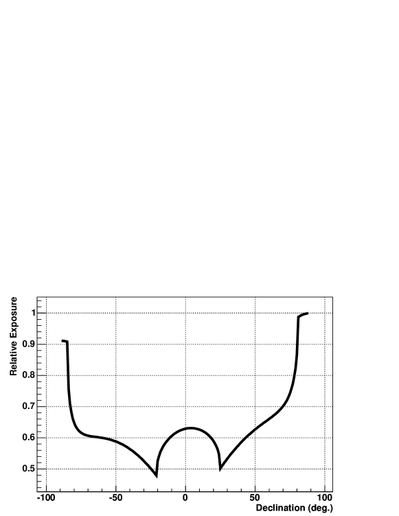
Figure 5: Relative exposure of the full Pierre Auger Observatory.

The base-line design of the detector includes a ground array consisting of 1600 water Čerenkov detectors overlooked by 4 fluorescence eyes. The angular and energy resolutions of the ground arrays are typically less than $1.5^{\circ}$ (multi-pole expansion $\ell\sim 60$) and less than 20%, respectively. The detectors are designed to be fully efficient ($p\approx 1$) out to $\theta_{\rm max}=60^{\circ}$ beyond $10^{19}$ eV, yielding a nearly uniform sky $A\approx 1.4\times 10^{4}$ km² sr.[33] In 10 yr of running the two arrays will collect $\approx 4000$ events above $E_{1}=10^{19.6}$ eV. As can be seen from Fig. 4, such statistics will allow one to discern asymmetries at the level of about 1 in $10^{4}$.

References

- [1] For recent reviews see e.g., P. Bhattacharjee and G. Sigl, Phys. Rept. 327, 109 (2000) [arXiv:astro-ph/9811011]; M. Nagano and A. A. Watson, Rev. Mod. Phys. 72 (2000) 689; L. Anchordoqui, T. Paul, S. Reucroft and J. Swain, Int. J. Mod. Phys. A 18, 2229 (2003) [arXiv:hep-ph/0206072].
- [2] K. Greisen, Phys. Rev. Lett. 16, 748 (1966); G. T. Zatsepin and V. A. Kuzmin, JETP Lett. 4, 78 (1966) [Pisma Zh. Eksp. Teor. Fiz. 4, 114 (1966)].
- [3] J. L. Puget, F. W. Stecker and J. H. Bredekamp, Astrophys. J. 205 (1976) 638.
- [4] J. Linsley, Phys. Rev. Lett. 10, 146 (1963).
- [5] M. Ave, J. A. Hinton, R. A. Vazquez, A. A. Watson and E. Zas, Phys. Rev. Lett. 85, 2244 (2000) [arXiv:astro-ph/0007386].
- [6] L. Anchordoqui and H. Goldberg, arXiv:hep-ph/0310054.
- [7] M. Takeda et al., Astropart. Phys. 19, 447 (2003) [arXiv:astro-ph/0209422].
- [8] D. J. Bird et al., Astrophys. J. 441, 144 (1995).
- [9] P. Bhattacharjee, C. T. Hill and D. N. Schramm, Phys. Rev. Lett. 69, 567 (1992).
- [10] V. Berezinsky, M. Kachelriess and A. Vilenkin, Phys. Rev. Lett. 79, 4302 (1997) [arXiv:astro-ph/9708217]; S. Sarkar and R. Toldra, Nucl. Phys. B 621, 495 (2002) [arXiv:hep-ph/0108098]; C. Barbot and M. Drees, Phys. Lett. B 533, 107 (2002) [arXiv:hep-ph/0202072].
- [11] R. J. Protheroe and T. Stanev, Phys. Rev. Lett. 77, 3708 (1996) [Erratum-ibid. 78, 3420 (1997)] [arXiv:astro-ph/9605036]; M. Ave, J. A. Hinton, R. A. Vazquez, A. A. Watson and E. Zas, Phys. Rev. D 65, 063007 (2002) [arXiv:astro-ph/0110613]; L. A. Anchordoqui, J. L. Feng, H. Goldberg and A. D. Shapere, Phys. Rev. D 66, 103002 (2002) [arXiv:hep-ph/0207139]. D. V. Semikoz and G. Sigl, arXiv:hep-ph/0309328.
- [12] G. R. Farrar, Phys. Rev. Lett. 76, 4111 (1996) [arXiv:hep-ph/9603271]; D. J. Chung, G. R. Farrar and E. W. Kolb, Phys. Rev. D 57, 4606 (1998) [arXiv:astro-ph/9707036]; V. Berezinsky, M. Kachelriess and S. Ostapchenko, Phys. Rev. D 65, 083004 (2002) [arXiv:astro-ph/0109026]; M. Kachelriess, D. V. Semikoz and M. A. Tortola, arXiv:hep-ph/0302161.
- [13] D. Fargion, B. Mele and A. Salis, Astrophys. J. 517, 725 (1999) [arXiv:astro-ph/9710029]; T. J. Weiler, Astropart. Phys. 11, 303 (1999) [arXiv:hep-ph/9710431]; S. R. Coleman and S. L. Glashow, arXiv:hep-ph/9808446; G. Domokos and S. Kovesi-Domokos, Phys. Rev. Lett. 82, 1366 (1999) [arXiv:hep-ph/9812260]; P. Jain, D. W. McKay, S. Panda and J. P. Ralston, Phys. Lett. B 484, 267 (2000) [arXiv:hep-ph/0001031]; C. Csaki, N. Kaloper, M. Peloso and J. Terning, arXiv:hep-ph/0302030; Z. Fodor, S. D. Katz, A. Ringwald and H. Tu, Phys. Lett. B 561, 191 (2003) [arXiv:hep-ph/0303080].
- [14] I. F. Albuquerque et al. [E761 Collaboration], Phys. Rev. Lett. 78, 3252 (1997) [arXiv:hep-ex/9604002]; A. Alavi-Harati et al. [KTeV Collaboration], Phys. Rev. Lett. 83, 2128 (1999) [arXiv:hep-ex/9903048].
- [15] M. Kachelriess and M. Plumacher, Phys. Rev. D 62, 103006 (2000) [arXiv:astro-ph/0005309]; L. Anchordoqui, H. Goldberg, T. McCauley, T. Paul, S. Reucroft and J. Swain, Phys. Rev. D 63, 124009 (2001) [arXiv:hep-ph/0011097]; R. Emparan, M. Masip and R. Rattazzi, Phys. Rev. D 65, 064023 (2002) [arXiv:hep-ph/0109287].
- [16] N. Hayashida et al., Phys. Rev. Lett. 77, 1000 (1996). Y. Uchihori, M. Nagano, M. Takeda, M. Teshima, J. Lloyd-Evans and A. A. Watson, Astropart. Phys. 13 (2000) 151 [arXiv:astro-ph/9908193]; P. G. Tinyakov and I. I. Tkachev, JETP Lett. 74, 1 (2001) [Pisma Zh. Eksp. Teor. Fiz. 74, 3 (2001)] [arXiv:astro-ph/0102101]; L. A. Anchordoqui, H. Goldberg, S. Reucroft, G. E. Romero, J. Swain and D. F. Torres, Mod. Phys. Lett. A 16, 2033 (2001) [arXiv:astro-ph/0106501].
- [17] V. Berezinsky and A. A. Mikhailov, Phys. Lett. B 449, 237 (1999) [arXiv:astro-ph/9810277]; P. Blasi, R. I. Epstein and A. V. Olinto, Astrophys. J. 533 (2000) L123 [arXiv:astro-ph/9912240].
- [18] N. Hayashida et al. [AGASA Collaboration], Astropart. Phys. 10, 303 (1999) [arXiv:astro-ph/9807045]; M. Takeda et al., arXiv:astro-ph/9902239.
- [19] J. A. Bellido, R. W. Clay, B. R. Dawson and M. Johnston-Hollitt, Astropart. Phys. 15, 167 (2001) [arXiv:astro-ph/0009039].
- [20] D. J. Bird et al. [HIRES Collaboration], arXiv:astro-ph/9806096.
- [21] L. A. Anchordoqui, H. Goldberg, F. Halzen and T. J. Weiler, arXiv:astro-ph/0311002.
- [22] T. Stanev, P. L. Biermann, J. Lloyd-Evans, J. P. Rachen and A. Watson, Phys. Rev. Lett. 75, 3056 (1995) [arXiv:astro-ph/9505093]; A. Smialkowski, M. Giller and W. Michalak, J. Phys. G 28, 1359 (2002) [arXiv:astro-ph/0203337]; D. F. Torres, E. Boldt, T. Hamilton and M. Loewenstein, Phys. Rev. D 66, 023001 (2002) [arXiv:astro-ph/0204419]; L. A. Anchordoqui, H. Goldberg and D. F. Torres, arXiv:astro-ph/0209546; C. Isola, G. Sigl and G. Bertone, arXiv:astro-ph/0312374.
- [23] G. R. Farrar and P. L. Biermann, Phys. Rev. Lett. 81, 3579 (1998) [arXiv:astro-ph/9806242]; G. Sigl, D. F. Torres, L. A. Anchordoqui and G. E. Romero, Phys. Rev. D 63, 081302 (2001) [arXiv:astro-ph/0008363]; A. Virmani, S. Bhattacharya, P. Jain, S. Razzaque, J. P. Ralston and D. W. McKay, Astropart. Phys. 17, 489 (2002) [arXiv:astro-ph/0010235]; P. G. Tinyakov and I. I. Tkachev, JETP Lett. 74, 445 (2001) [Pisma Zh. Eksp. Teor. Fiz. 74, 499 (2001)] [arXiv:astro-ph/0102476]; W. Evans, F. Ferrer and S. Sarkar, arXiv:astro-ph/0212533; D. F. Torres, S. Reucroft, O. Reimer and L. A. Anchordoqui, Astrophys. J. 595, L13 (2003) [arXiv:astro-ph/0307079].
- [24] P. J. E. Peebles, Astrophys. J. 185, 413 (1973); M. G. Hauser and P. J. E. Peebles, Astrophys. J. 185, 757 (1973); M. Tegmark, D. H. Hartmann, M. S. Briggs and C. A. Meegan, Astrophys. J. 468 (1996) 214 [arXiv:astro-ph/9510129].
- [25] L. A. Anchordoqui, C. Hojvat, T. P. McCauley, T. C. Paul, S. Reucroft, J. D. Swain and A. Widom, Phys. Rev. D 68, 083004 (2003) [arXiv:astro-ph/0305158].
- [26] C. Hojvat, T. P. McCauley, S. Reucroft and J. D. Swain, arXiv:astro-ph/0305206.
- [27] M. M. Winn, J. Ulrichs, L. S. Peak, C. B. Mccusker and L. Horton, J. Phys. G 12 (1986) 653.
- [28] R. W. Clay, R. Meyhandan, L. Horton, J. Ulrichs, and M. M. Winn, Astron. Astrophys. 255, 167 (1992); L. J. Kewley, R. W. Clay and B. R. Dawson, Astropart. Phys. 5, 69 (1996).
- [29] C. J. Bell et al., J. Phys. A 7 (1974) 990.
- [30] N. Chiba et al., Nucl. Instrum. Meth. A 311, 338 (1992); H. Ohoka, S. Yoshida and M. Takeda [AGASA Collaboration], Nucl. Instrum. Meth. A 385, 268 (1997).
- [31] M. Teshima et al., Nucl. Instrum. Meth. A 247, 399 (1986).
- [32] M. Takeda et al., Phys. Rev. Lett. 81, 1163 (1998) [arXiv:astro-ph/9807193].
- [33] P. Sommers, Astropart. Phys. 14, 271 (2001) [arXiv:astro-ph/0004016].
- [34] N. Hayashida et al., arXiv:astro-ph/0008102.
- [35] For this analysis we use real-valued spherical harmonics, which are obtained from the complex ones by substituting, , if , , if , and if These are discussed again in more detail in section 4.1 where the fact that they are real is of paramount importance in constructing a real–valued likelihood function.
- [36] C. Isola and G. Sigl, Phys. Rev. D 66, 083002 (2002) [arXiv:astro-ph/0203273]; M. Kachelriess and D. V. Semikoz, arXiv:astro-ph/0306282.
- [37] T. Abu-Zayyad et al. [High Resolution Fly’s Eye Collaboration], arXiv:astro-ph/0208243.
- [38] http://www.auger.org
- [39] J. Abraham et al, [AUGER Collaboration], Nucl. Inst. Meth. A (to be published in 2004).
- [40] Carlos Hojvat, Thomas P. McCauley, Stephen Reucroft, John D. Swain, arXiv:astro-ph/0305206, FERMILAB-CONF-03-185-A, published in Proceedings of 28th International Cosmic Ray Conferences (ICRC 2003), Tsukuba, Japan, 31 Jul – 7 Aug 2003.
- [41] Edwards, A. W. F., “Likehood”, Cambridge University Press, Cambridge, 1972.
- [42] Carl Sagan, Linda Salzman Sagan, and Frank Drake, Science 175 (1972) 881.
- [43] http://www.seti-inst.edu/
- [44] http://www.coseti.org/opticals.htm