The 2dF Galaxy Redshift Survey: Higher order galaxy correlation functions

Abstract

We measure moments of the galaxy count probability distribution function in the two-degree field galaxy redshift survey (2dFGRS). The survey is divided into volume limited subsamples in order to examine the dependence of the higher order clustering on galaxy luminosity. We demonstrate the hierarchical scaling of the averaged $p$-point galaxy correlation functions, $\bar{\xi}_{p}$, up to $p=6$. The hierarchical amplitudes, $S_{p}=\bar{\xi}_{p}/\bar{\xi}_{2}^{p-1}$, are approximately independent of the cell radius used to smooth the galaxy distribution on small to medium scales. On larger scales we find the higher order moments can be strongly affected by the presence of rare, massive superstructures in the galaxy distribution. The skewness $S_{3}$ has a weak dependence on luminosity, approximated by a linear dependence on log luminosity. We discuss the implications of our results for simple models of linear and non-linear bias that relate the galaxy distribution to the underlying mass.

1 Introduction

The pattern of galaxy clustering can be quantified by measuring the galaxy count probability distribution function (CPDF) on a range of smoothing scales. The CPDF gives the probability that a randomly chosen region of the universe will contain a particular number of galaxies, and is typically expressed as a function of both the size of the region smoothed over and the galaxy number within that volume. Traditionally, most effort has been directed at measuring the second moment of the count distribution, the variance, $\bar{\xi}_{2}$, through the autocorrelation function or, equivalently, its Fourier transform, the power spectrum (e.g. Percival et al. 2001; Padilla & Baugh 2003; Tegmark et al. 2004). The higher order moments of the CPDF, expressed as volume averaged correlation functions, $\bar{\xi}_{p}$ ($p=2,3,\dots$), provide a much more detailed description of galaxy clustering, probing the shape of the low and high count tails of the distribution.

The higher order moments of the dark matter distribution are known to display a hierarchical scaling in which the $p$-point volume averaged correlation functions, $\bar{\xi}_{p}$, can be written in terms of the variance of the count distribution, $\bar{\xi}_{2}$: $\bar{\xi}_{p}=S_{p}\bar{\xi}^{p-1}_{2}$ (e.g. see Peebles 1980, Juszkiewicz, Bouchet & Colombi 1993, Bernardeau 1994, Baugh, Gaztañaga & Efstathiou 1995, Gaztañaga & Baugh 1995, Fosalba & Gaztañaga 1998). This scaling is a signature of the evolution under gravitational instability of an initially Gaussian distribution of density fluctuations. A remarkable feature of the scaling is that the values of the hierarchical amplitudes, $S_{p}$, on scales for which the density field evolves linearly or in a quasi-linear fashion, are insensitive to cosmic epoch and essentially independent of the cosmological density parameter or the value of the cosmological constant. For a comprehensive review of such results see Bernardeau et al. (2002) and references therein.

Departures from the hierarchical scaling of the higher order moments could conceivably arise in three ways:

• A strongly non-Gaussian distribution of primordial density waves as could arise, for instance, due to a seed non-linear fluctuation such as a global texture (see Gaztañaga & Mahonen 1996, Gaztañaga & Fosalba 1998, Scoccimarro, Sefusatti & Zaldarriaga 2003 for examples of how the $S_{p}$ scale in this case). This avenue now seems unlikely, following the clear detection of multiple acoustic peaks in the power spectrum of cosmic microwave background temperature fluctuations (Netterfield et al. 2002; Hinshaw et al. 2003; Mason et al. 2003; Scott et al. 2003; Kuo et al. 2004); such peaks are difficult to reconcile with models that include cosmological defects (Kamionkowski & Kowsowsky 1999). Moreover strongly non-Gaussian primordial fluctuations are ruled out by the first year WMAP results (Komatsu et al. 2003; Gaztañaga & Wagg 2003)

• A weakly non-Gaussian distributed primordial density field, resulting from a non-linear perturbation to a Gaussian density field. This scenario is difficult to distinguish from the evolution of an initially Gaussian field under gravitational instability, because the perturbation can introduce a shift to the amplitudes $S_{p}$ that is also hierarchical. This can happen even in the case where the non-linear perturbation produces a negligible effect on the power spectrum (Bernardeau et al. 2002).

• The spatial bias between the galaxy distribution and the underlying distribution of dark matter. Fry & Gaztañaga (1993) demonstrated that, under a local biasing prescription, the hierarchical scaling of the higher order moments is preserved but the amplitudes $S_{p}$ can change as a function of time or luminosity. This conclusion is also reached using more sophisticated, physically motivated semi-analytic models of galaxy formation (Kauffmann et al. 1999; Benson et al. 2000; Scoccimarro et al. 2001).

Previous attempts to measure the higher order correlation functions have been hamstrung by the small size of the available redshift surveys, a shortcoming that is exacerbated once volume limited subsamples are constructed (Hui & Gaztañaga 1999). Nevertheless, early counts-in-cells studies established that the first few higher order moments of the galaxy distribution displayed the hierarchical scaling expected in the gravitational instability framework (Groth & Peebles 1977; Peebles 1980; Gaztañaga 1992; Bouchet et al. 1993; Fry & Gaztañaga 1994, Ghigna et al. 1996, Feldman et al. 2001). Such analyses were typically limited to measuring the three and four point correlation functions. The nature of the dependence of the hierarchical amplitudes on luminosity has not been convincingly established. Recent work to investigate this in the optical (Hoyle et al. 2000) and in the far infrared (Szapudi et al. 2000) was restricted to probing fairly narrow ranges of luminosity due to the size of the redshift surveys then available.

The advent of multi-fibre spectrographs exploited by sustained observing campaigns has led to a new generation of redshift survey which represents order of magnitude advances over surveys completed in the last millennium. The Sloan Digital Sky Survey (York et al. 2000) and the Two-degree Field Galaxy Redshift Survey (2dFGRS, Colless et al. 2001) have provided maps of the clustering pattern of galaxies with unprecedented detail. Analysis of the 2dFGRS clustering has suggested that the flux limited sample could be an essentially unbiased tracer of the dark matter in the Universe (Lahav et al. 2002; Verde et al. 2002) . These results confirmed previous deductions about galaxy bias (e.g. Gaztañaga 1994, Frieman & Gaztañaga 1999, Gaztañaga & Juszkiewicz 2001) reached using the parent angular catalogue of the 2dFGRS, the APM Galaxy Survey (Maddox et al. 1990, 1996). The 2dFGRS covers a volume that is an appreciable fraction of that sampled by the APM Survey, with full redshift coverage (modulo the relatively small redshift incompleteness that still remains). This means that for the first time, a measurement of the higher order moments is possible in three dimensions with comparable accuracy to that attainable in two dimensions, but without the added complication of the effects of projection (Bernardeau & Gaztañaga 1996; Szapudi & Gaztañaga 1998).

The sheer number of galaxies in the 2dFGRS allows it to be subdivided in order to probe the dependence of the clustering signal on intrinsic galaxy properties in more detail. Norberg et al. (2001) found that the amplitude of the projected two point correlation function scales with luminosity, and characterised this trend using a relative bias factor with a linear dependence on luminosity. In this paper we extend the work of Norberg et al. to study the higher order clustering of galaxies in the 2dFGRS and its dependence on luminosity. Our approach is the same as that followed in Baugh et al. (2004), who measured the higher order correlation functions of a sample of $L_{*}$ galaxies and found that they follow a hierarchical scaling.

We provide a brief review of the measurement of the moments of the CPDF in Section 2. In Section 3, we discuss the specific application of this method to the 2dFGRS; an important feature of our analysis is the use of mock catalogues to estimate the errors on our measurements (see Section 3.3). Our results for the higher order correlation functions and the hierarchical amplitudes are given in Section 4. We quantify the variation of the higher order moments with luminosity in Section 5, and discuss the interpretation of these results in terms of a simple relative bias model. Our conclusions are set out in Section 6. Throughout, we adopt standard present day values of the cosmological parameters to compute comoving distance from redshift: a density parameter $\Omega_{m}=0.3$ and a cosmological constant $\Omega_{\Lambda}=0.7$.

2 Count-in-Cells Statistics

The count probability distribution function (CPDF) and its moments have been used extensively to quantify the clustering pattern of galaxies (e.g. White 1979; Peebles 1980). In this Section we give an outline of the counts-in-cells approach, explaining how the volume averaged $p$-point correlations are derived from the CPDF and give a brief theoretical background. A more comprehensive discussion of the counts-in-cells approach can be found in Bernardeau et al. (2002).

2.1 Estimating the $p$-point volume averaged correlation functions

The $p$-point moment, or (un-reduced) correlation function, $m_{3}(r_{1},r_{2},r_{3})\equiv<\delta(r_{1})...\delta(r_{p})>$, can be used to fully characterise the clustering of a fluctuating field $\delta(r)$. The reduced $p$-point correlation function, $\xi_{p}(r_{1},...,r_{p})$, is defined as the connected part of the above $p$-point correlation in such a way that for $p>2$: $\xi_{p}=0$ for a Gaussian field (see Bernardeau et al. 2002 for more details). Following the standard convention, for the remainder of this paper when we talk about correlations we will always assume they are “reduced” correlations.

The $p$-point volume averaged galaxy correlation function, $\bar{\xi}_{p}(V)$, can be written as the integral of the $p$-point correlation function, $\xi_{p}$, over the sampling volume, $V$ (Peebles 1980):

$$\bar{\xi}_{p}(V)=\frac{1}{V^{p}}\int_{V}{\rm d}^{3}r_{1}\ \dots\ {\rm d}^{3}r_{p}\ \xi_{p}(\mathbf{r_{1}},\ \dots\ ,\mathbf{r_{p}})~{}.$$ (1)

A practical way in which to estimate $\bar{\xi}_{p}(V)$ is to randomly throw cells down within the galaxy distribution, recording the number of times a cell contains $N$ galaxies so as to build up the galaxy CPDF, $P_{N}(V)$. Since we adopt spherical cells, the CPDF is a function of the sphere radius, $R$,

$$P_{N}(R)=\frac{N_{N}}{N_{T}}~{},$$ (2)

where $N_{N}$ is the number of cells that contain $N$ galaxies out of a total number of cells thrown down, $N_{T}$. The volume averaged correlation functions $\bar{\xi}_{p}(V)$ are then related to the moments of the CPDF, $m_{p}$:

$$m_{p}(R)=\langle(N-\bar{N})^{p}\rangle=\sum_{N=0}^{\infty}P_{N}(R)(N-\bar{N})^{p}~{},$$ (3)

where $\bar{N}$ is the mean number of galaxies in a cell of volume $V$ and is calculated directly from the CPDF

$$\bar{N}=\sum_{N=0}^{\infty}NP_{N}~{}.$$ (4)

For the case of a continuous distribution, $\bar{\xi}_{p}$ is related to the corresponding cumulant, $\mu_{p}$, through $\bar{N}^{p}\bar{\xi}_{p}=\mu_{p}$, where the cumulants are defined as (see Gaztañaga 1994 for details):

$$\mu_{2}=m_{2}~{}~{}~{}~{};~{}~{}~{}\mu_{3}=m_{3}~{},$$

$$\mu_{4}=m_{4}-3m_{2}^{2}~{}~{}~{}~{};~{}~{}~{}\mu_{5}=m_{5}-10m_{3}m_{2}~{}.$$ (5)

If instead we are dealing with a discrete distribution, these relations must be corrected. A Poisson shot noise model is adopted (see Baugh et al. 1995 for a discussion of this point), to give corrected estimates of the moments, $k_{p}$:

$$k_{2}=\mu_{2}-\bar{N}~{}~{}~{};~{}~{}~{}k_{3}=\mu_{3}-3k_{2}-\bar{N}~{},$$

$$k_{4}=\mu_{4}-7k_{2}-6k_{3}-\bar{N}~{},$$

$$k_{5}=\mu_{5}-15k_{2}-25k_{3}-10k_{4}-\bar{N}~{}.$$ (6)

The volume-averaged correlation functions, calculated from the galaxy CPDF, follow directly from the relation $\bar{\xi}_{p}=k_{p}/\bar{N}^{p}$.

2.2 Scaling of the higher order moments

In the hierarchical model of clustering, all higher-order correlations can be expressed in terms of the 2-point function, $\bar{\xi}_{2}$, and dimensionless scaling coefficients, $S_{p}$:

$$\bar{\xi}_{p}=S_{p}~{}\bar{\xi}_{2}^{p-1}.$$ (7)

Traditionally, $S_{3}=\bar{\xi}_{3}/\bar{\xi}_{2}^{2}$ is referred to as the skewness of the distribution and $S_{4}=\bar{\xi}_{4}/\bar{\xi}_{2}^{3}$ as the kurtosis. The hierarchical scaling of the higher order moments arises from the evolution due to gravitational instability of an initially Gaussian distribution of density fluctuations (see Bernardeau et al. 2002 and references therein).

2.3 Systematic effects: biased estimators

In addition to sampling errors (see Section 3.3 below), the estimation of the hierarchical amplitudes can be compromised by systematic effects, as discussed in some detail by Hui & Gaztañaga (1999). These authors identified two sources of error that could lead to a systematic bias in the inferred values of $S_{p}$. The first effect arises from biases in the estimates of the higher order correlation functions themselves, known as the “integral constraint bias” (see e.g. Bernstein 1994). The second effect originates in the nonlinear combination of $\bar{\xi}_{p}$ and $\bar{\xi}_{2}$ to form $S_{p}$; this is called the “ratio bias”. The latter effect dominates on large scales and tends to cause the inferred values of the $S_{p}$ to be biased low. Hui & Gaztañaga wrote down expressions for these biases which accurately reproduce the systematic effects seen upon estimating the hierarchical amplitudes from sub-volumes extracted from N-body simulations.

As mentioned above, we will use different volume limited samples to study the luminosity dependence of the hierarchical amplitudes, $S_{p}$. As the luminosity that defines a sample is made brighter, the volume of the sample increases. Thus the estimation biases tend to cause the $S_{p}$ to increase with sample luminosity. This spurious tendency has already been reported in the literature (see Hui & Gaztañaga 1999). For volumes of the size used in our analysis, it turns out that the predicted biases are smaller than the corresponding sampling errors (e.g. see figure 3 in Hui & Gaztañaga 1999). This is the first time that a redshift survey has been available which is large enough to overcome such systematic biases.

2.4 Galaxy biasing

Galaxy samples constructed using different selection criteria display different clustering patterns. This leads one to the conclusion that distinct samples of galaxies must trace the underlying mass distribution in different ways, a phenomenon that is generally known as galaxy bias.

A simple, heuristic scheme describing the impact of a local bias on the scaling of the higher order moments was proposed by Fry & Gaztañaga (1993). These authors demonstrated that in this case, the scaling of the higher order moments of the galaxy distribution should mirror that of the dark matter, though possibly with different values for the hierarchical amplitudes $S_{p}$. Fry & Gaztañaga made the assumption that the density contrast in the galaxy distribution, $\delta^{\rm G}$, i.e. the fractional fluctuation around the mean density, could be written as a Taylor expansion of the density contrast of the dark matter, $\delta^{\rm DM}$:

$$\delta^{\rm G}=\sum_{k=0}^{\infty}\frac{b_{k}}{k!}(\delta^{\rm DM})^{k}.$$ (8)

On scales where the variance, $\bar{\xi}_{2}^{\rm DM}$, is small, the leading order contribution to the two-point volume averaged correlation function of galaxies has the form:

$$\bar{\xi}^{\rm G}_{2}=b_{1}^{2}~{}\bar{\xi}^{\rm DM}_{2},$$ (9)

where $b_{1}$ is the ubiquitous linear bias $b$. The leading order forms for the hierarchical amplitudes, $S_{p}$, for the cases $p=3$ and $p=4$ are:

$$S^{\rm G}_{3} = \frac{1}{b_{1}}\left(S^{\rm DM}_{3}+3c_{2}\right)$$ (10)

$$S^{\rm G}_{4} = \frac{1}{b_{1}^{2}}\left(S^{\rm DM}_{4}+12c_{2}S^{\rm DM}_{3}+4c_{3}+12c^{2}_{2}\right),$$ (11)

where we use the notation $c_{k}=b_{k}/b_{1}$. Expressions for the hierarchical amplitudes are given up to $p=7$ in Fry & Gaztañaga (1993).

Mo, Jing & White (1997) give theoretical predictions for the coefficients $b_{k}$ using the Press & Schechter (1974) formalism and exploiting the framework developed by Cole & Kaiser (1989) and Mo & White (1996). For halos of mass $M$, the first two bias factors ($k=1$ and 2) are given by:

$$b_{1}=1+{\nu^{2}-1\over\delta_{c}}$$ (12)

$$b_{2}=2\left(1-{17\over 21}\right){\nu^{2}-1\over\delta_{c}}+{\nu^{2}\over\delta_{c}^{2}}(\nu^{2}-3)$$ (13)

where $\nu\equiv\delta_{c}/\sigma(M)$, $\delta_{c}$ is the linear theory overdensity at the time of collapse ($\delta_{c}=1.686$ for $\Omega=1$) and $\sigma(M)$ is the linear rms fluctuation on the mass scale of the halos. This is a simple model but nevertheless it shows some tendencies that are correct. For example, a typical mass halo corresponding to $\nu=1$ displays an unbiased variance with $b_{1}=1$, but introduces a bias in the skewness, since $c_{2}=b_{2}=-0.7$. As a further illustration, consider massive halos defined by $\nu^{2}>3$; in this case the Mo, Jing & White theory predicts that $c_{2}>0$, while less massive halos could produce $c_{2}<0$. To get more realistic values of $b_{k}$ for galaxy bias, a prescription has to be adopted for populating dark matter halos of a given mass with galaxies of a given luminosity (Benson et al. 2001; Scoccimarro et al. 2001; Berlind et al. 2003).

In the interpretation of the higher order moments presented in this paper we will make use of a relative bias, which describes the change in clustering compared with that measured for a reference sample (Norberg et al. 2001, 2002a). Using Eq. 9 as a guide, we define the relative bias, $b_{r}=b_{1}/b^{*}_{1}$, of a sample as the square root of the ratio of the $2$-point correlation function measured for the sample over that measured for the reference sample, denoted by an asterisk (the reference sample will be defined explicitly in Section 5):

$$b_{r}\equiv{b_{1}\over{b^{*}_{1}}}=\Big{(}\frac{\bar{\xi}^{G}_{2}}{\bar{\xi}^{G*}_{2}}\Big{)}^{1/2}.$$ (14)

Thus, we can obtain an estimate of the relative bias from the ratio of the variances.

When the linear bias is a good approximation ($c_{k}\simeq 0$ for $k>1$), we can relate $S_{p}^{G}$ in different galaxy samples regardless of the underlying DM value of $S_{p}$:

$$S^{G}_{p}=\frac{S^{G*}_{p}}{b^{p-2}_{r}}.$$ (15)

More generally, one can manipulate Eq. 10 to write down an expression comparing $S_{p}^{G}$ for two galaxy samples, eliminating $S_{3}^{\rm DM}$ for the underlying dark matter (e.g. see Eq. 9 in Fry & Gaztañaga 1993). For the skewness:

$$S^{G*}_{3}=b_{r}S^{G}_{3}-3\frac{(c_{2}-c^{*}_{2})}{b_{1}^{*}}~{},$$ (16)

where an asterisk denotes a quantity describing the reference sample, and $b_{r}=b_{1}/b^{*}_{1}$ is the relative bias defined above. Any second order relative bias effects are thus given by:

$$c_{2}^{\prime}=\frac{(c_{2}-c^{*}_{2})}{b_{1}^{*}}=\frac{1}{3}\left(b_{r}S^{G}_{3}-S^{G*}_{3}\right).$$ (17)

As a special case, if the reference sample is un-biased (i.e. $b_{1}^{*}=1$ and $c_{p}^{*}=0$), we then have $c_{2}^{\prime}=c_{2}$.

Table 1: Properties of the combined 2dFGRS SGP and NGP volume-limited catalogues (VLCs). Column 1 gives the numerical label of the sample. Columns 2 and 3 give the faint and bright absolute magnitude limits that define the sample. The fourth column gives the median luminosity of each volume limited sample in units of $L_{*}$, computed using the Schechter function parameters quoted by Norberg et al. (2002b). Columns 5, 6 and 7 give the number of galaxies, the mean number density and the mean inter-galaxy separation for each VLC, respectively. Columns 8 and 9 state the redshift boundaries of each sample for the nominal apparent magnitude limits of the survey; columns 10 and 11 give the corresponding comoving distances. Finally, column 12 gives the combined SGP and NGP volume. All distances are comoving and are calculated assuming standard cosmological parameters ($\Omega_{m}=0.3$ and $\Omega_{\Lambda}=0.7$).

VLC	Mag. range		Median lum.	NG	$\rho_{\rm ave}$	dmean	zmin	zmax	Dmin	Dmax	Volume
ID	$M_{b_{\rm J}}-5\log_{10}h$		$L/L_{*}$		$10^{-3}h^{3}$Mpc-3	$h^{-1}$Mpc			$h^{-1}$Mpc	$h^{-1}$Mpc	$10^{6}h^{-3}$Mpc3
1	$-$17.0	$-$18.0	0.13	8038	10.9	4.51	0.009	0.058	24.8	169.9	0.74
2	$-$18.0	$-$19.0	0.33	23290	9.26	4.76	0.014	0.088	39.0	255.6	2.52
3	$-$19.0	$-$20.0	0.78	44931	5.64	5.62	0.021	0.130	61.1	375.6	7.97
4	$-$20.0	$-$21.0	1.78	33997	1.46	8.82	0.033	0.188	95.1	537.2	23.3
5	$-$21.0	$-$22.0	3.98	6895	0.110	20.9	0.050	0.266	146.4	747.9	62.8

Table 2: The best fit values and 2$-\sigma$ error ($\Delta\chi^{2}=4$) for $S_{p}$ (columns 4 to 7). The range of scales used in the fits is given in columns 2 and 3. The number in brackets after each error gives the reduced $\chi^{2}$ value for the fit, using the number of degrees of freedom derived from the principal component analysis. The last two columns give the relative linear bias, $b_{r}$ (defined by Eq. 14) and the second order bias term, $c_{2}^{\prime}$ (defined by Eq. 17). The reference sample is sample number 3. These values are obtained for the full volume limited samples. A blank entry indicates that a reliable measurement of the particular hierarchical amplitude was not possible for the sample in question.

VLC	$R_{\rm min}$	$R_{\rm max}$	$S_{3}$	$S_{4}$	$S_{5}$	${S_{6}}$	$b_{r}$	$c_{2}^{\prime}$
ID	$h^{-1}$Mpc	$h^{-1}$Mpc
1	0.71	7.1	$2.58\pm 0.37\,(0.1)$	$9.3\pm 4.0\,(0.1)$	$34\pm 32\,(0.1)$	$---$	$0.96\pm 0.16\,(0.1)$	$0.17\pm 0.25\,(0.1)$
2	0.71	7.1	$2.38\pm 0.25\,(0.1)$	$8.2\pm 2.3\,(0.9)$	$36\pm 20\,(0.4)$	$185\pm 170(0.1)$	$0.96\pm 0.08\,(0.3)$	$0.11\pm 0.13\,(0.1)$
3	0.71	7.1	$1.95\pm 0.18\,(6.1)$	$5.5\pm 1.4\,(2.3)$	$18\pm 11\,(1.9)$	$46\pm 50(1.1)$	$1$	$0$
4	0.80	8.9	$2.01\pm 0.17\,(1.2)$	$6.0\pm 1.5\,(0.6)$	$22\pm 12\,(0.4)$	$71\pm 80(0.3)$	$1.13\pm 0.06\,(2.8)$	$0.10\pm 0.08\,(0.3)$
5	2.2	11.2	$2.39\pm 0.63\,(0.5)$	$6.8\pm 7.0\,(0.4)$	$---$	$---$	$1.30\pm 0.14\,(0.9)$	$0.33\pm 0.31\,(0.5)$

3 Application to the 2dFGRS

In this Section we describe the construction of volume limited samples from the 2dFGRS (Section 3.1) and outline how we deal with the small, remaining incompleteness of the survey when we measure the CPDF (Section 3.2). The estimation of errors on the measured higher order moments is described in Section 3.3. We use the full 2dFGRS as our starting point. The final spectra were taken in April 2002, giving a total of 221,414 galaxies with high quality redshifts (i.e. with quality flag Q $\geq 3$; see Colless et al. 2001). The median depth of the full survey, to a nominal magnitude limit of $b_{\rm J}\sim 19.45$, is $z\sim 0.11$. We consider the two large contiguous survey regions, one near the south galactic pole (SGP) and the other towards the north galactic pole (NGP). After restricting attention to the high redshift completeness parts of the survey (see Colless et al. 2001; Norberg et al. 2002b), the effective solid angle covered by the NGP region is 469 square degrees and that of the SGP is 670 square degrees. Full details of the 2dFGRS and the construction and use of the mask quantifying the completeness of the survey can be found in Colless et al. (2001, 2003).

We make use of mock 2dFGRS catalogues to test our algorithm for dealing with the spectroscopic incompleteness of the survey and to estimate errors on the measured higher order correlation functions. The construction of the mocks is described in Norberg et al. (2002b). In short, catalogues are extracted from the Virgo Consortium’s $\Lambda$CDM Hubble Volume simulation which covers a volume of $27{\rm Gpc}^{3}$ (Evrard et al. 2002). A heuristic bias scheme is applied to the smoothed distribution of dark matter in the simulation to select ‘galaxies’ with a specified clustering pattern (Cole et al. 1998). The parameters of the biasing scheme are adjusted so that the extracted galaxies have the same projected correlation function as measured for the flux limited 2dFGRS by Hawkins et al. (2003). Observers are placed within the Hubble Volume simulation according to the criteria set out in Norberg et al. (2002b). Mock catalogues are then extracted by applying the radial and angular selection functions of the 2dFGRS. Finally, the mock is degraded from uniform coverage within the angular mask of the survey by applying the spectroscopic completeness mask of the 2dFGRS.

3.1 Construction of volume limited catalogues

In a flux limited sample the density of galaxies is a strong function of radial distance. This effect needs to be taken into account in clustering analyses (for an example of a technique appropriate to a counts-in-cells analysis, see Efstathiou et al. 1990). Alternatively, one may construct volume limited samples in which the radial selection function is constant and any variations in the density of galaxies are due only to large scale structure. This greatly simplifies the analysis at the expense of using a subset of the survey galaxies. The 2dFGRS contains enough galaxies and covers sufficient volume to permit the construction of volume limited samples corresponding to a wide baseline in luminosity from which robust measurements of the higher order correlation functions can be obtained.

We follow the approach taken by Norberg et al. (2001, 2002a) who measured the projected 2-point correlation function of 2dFGRS galaxies in volume limited samples corresponding to bins in absolute magnitude. The samples are defined by a specified absolute magnitude range, with absolute magnitudes corrected to zero redshift (this correction is made using the $k+e$ correction given by Norberg et al. 2002b). As any survey has, in practice, a bright as well as a faint flux limit, this implies that a selected galaxy should fall between a minimum ($z_{\rm min}$) and a maximum ($z_{\rm max}$) redshift. This then guarantees that all sample galaxies are visible within the flux limits of the survey when displaced to any depth within the volume of the sample. The properties of the combined NGP and SGP volume limited samples examined in this paper are given in Table 1.

3.2 Correcting for incompleteness

Figure 1: A test of the scheme used to correct the measured distribution of counts-in-cells for incompleteness in the 2dFGRS, using mock catalogues. The plot shows the hierarchical amplitudes, $S_{p}$, for orders $p=3,4$ and $5$. The dotted lines show the results from fully sampled mocks that have no incompleteness. The dashed lines show how these results change when the completeness mask of the 2dFGRS is applied to the mocks and no compensation is made for the variable spectroscopic completeness. The circles show the $S_{p}$ recovered once the correction to the cell radius discussed in the text is made. The errorbars show the rms scatter estimated from the mock catalogues.

There are two possible sources of incompleteness that need to be considered when estimating the galaxy count within a cell. The first is volume incompleteness, which can arise when some fraction of the cell volume samples a region of space that is not part of the 2dFGRS. This situation can arise because the survey has a complicated boundary and also because it contains holes excised around bright stars and other interlopers in the parent APM galaxy catalogue (Maddox et al. 1990, 1996). The second source of incompleteness is spectroscopic incompleteness. The final 2dFGRS catalogue is much more homogeneous than the 100k release (contrast the completeness mask of the final survey shown in figure 1 of Hawkins et al. 2003 with the equivalent mask depicted in figure 15 of Colless et al. 2001.) However, the spectroscopic completeness still varies with position on the sky and needs to be incorporated into the counts-in-cells analysis.

It is therefore necessary to devise a strategy to compensate for the fact that a cell will sample regions that have varying spectroscopic completeness and which may even straddle the survey boundary or a hole. We project the volume enclosed by the cell onto the sky and estimate, using the survey masks, the mean combined spectroscopic and volume completeness, $f$, within the sphere. Rather than view the consequence of this incompleteness as missed galaxies, we instead consider it as missed volume. We compute a new radius for the sphere given by $R^{\prime}=f^{-\frac{1}{3}}R$: such a sphere with radius $R^{\prime}$ will have an incomplete volume equivalent to that of a fully complete sphere of radius $R$. Spheres for which $f$ is less than $50\%$ are discarded. The galaxy count within the sphere of radius $R^{\prime}$ then contributes to the CPDF at the effective radius $R$. Each sphere thrown down is individually scaled in this way according to its local incompleteness, as given by the survey masks. We note that, due to our chosen acceptable minimum completeness of $50\%$, the rescaling of the cell radius is always less than the width of the radial bins we use to plot the higher order correlation functions. Our results are insensitive to the precise choice of completeness threshold.

An alternative method to correct cell counts is described in Efstathiou et al. (1990). In this commonly used approach it is the galaxy counts which are scaled up in proportion to the degree of incompleteness in the cell, as opposed to the cell volume as we have done. We have tried both correction methods when calculating the higher order moments and find the results are essentially identical (see Croton et al. 2004 for further discussion of the relative strengths and weaknesses of both methods).

A test of our method for dealing with incompleteness is shown in Fig. 1. This plot shows the $S_{p}$ estimated from the higher order correlation functions measured in mock 2dFGRS catalogues (Norberg et al. 2002b). The dotted lines show the results for complete mocks, with uniform sampling of the galaxy distribution within the full angular boundary of the 2dFGRS. The dashed lines show how these results change once the mocks are degraded to mimic the spectroscopic incompleteness and irregular geometry of the 2dFGRS, without applying any correction to compensate for this incompleteness. The circles show the values of $S_{p}$ recovered on application of the correction for incompleteness described above. These results are in excellent agreement with those from the fully sampled, ‘perfect’ mocks.

We have carried out two independent counts-in-cells analyses, using different algorithms to place cells within the survey volume. The results are insensitive to the details of the counts-in-cells algorithm. The CPDF is measured using $2.5\times 10^{7}$ cells for each cell radius. We have further checked the counts in cells analysis by comparing the measured two point volume averaged correlation function with the integral of the measured spatial two point correlation function, given by Eq. 1; the integral of the spatial correlation function is in very good agreement with the direct estimate of the volume averaged correlation function.

3.3 Error Estimation

We estimate the error on the higher order correlation functions and hierarchical amplitudes using the set of 22 mock 2dFGRS surveys described by Norberg et al. (2002b). The $1\sigma$ errors that we show on plots correspond to the rms scatter over the ensemble of mocks (see Norberg et al. 2001a). To recap, we consider one of the mocks as the “data” and compute the variance around this “mean” using the remaining mock catalogues. This process is repeated for each mock in turn, and the rms scatter is taken as the mean variance. We illustrate this approach in Fig. 2 for the case of $p=3$, for a volume defined by the magnitude range $-19>M_{b_{\rm J}}-5\log_{10}h>-20$. In the upper panel, the skewness or $S_{3}$ measured in each mock is shown by the dotted lines. The points show the mean skewness averaged over the ensemble of 22 mocks. The errorbars show the rms scatter on these measurements. The lower panel shows the fractional error that we expect on the measurement of $S_{3}$ for this particular volume limited sample. Beyond $20h^{-1}$Mpc, the fractional error increases rapidly. Our estimate of the fractional error automatically includes the contribution from sampling variance due to large scale structure (sometimes referred to as “cosmic variance”). To estimate the error on a measured correlation function, we simply compute the fractional rms scatter for the equivalent volume limited sample using the ensemble of mocks, and multiply the measured quantity by the fractional error.

Figure 2: The upper panel shows the skewness, $S_{3}$, recovered from mock 2dFGRS catalogues in volume limited samples defined by the magnitude range $-19>M_{b_{\rm J}}-5\log_{10}h>-20$. The dotted lines show the skewness measured in each catalogue. The points show the mean skewness. The errorbars show the mean rms scatter averaged over 22 mocks, as described in the text in Section 3.3. The lower panel shows the fractional error as a function of cell radius. This panel shows how well we can expect to measure the skewness in a catalogue of this size extracted from the 2dFGRS, including the contribution from sampling variance.

We have compared the estimate of the rms scatter from the ensemble of mocks with an internal estimate using a jackknife technique (see, for example, Zehavi et al. 2002). In the jackknife approach, the survey is split into subsamples. The error is then the scatter between the measurements when each subsample is omitted in turn from the analysis. The jackknife gives comparable errors to the mock ensemble for low order moments. On large scales, the higher order moments are particularly sensitive to sample variance and, in these cases, the jackknife approach can only provide a lower bound to the true scatter.

A more formal error estimation procedure is adopted when computing the best fit values for the hierarchical amplitudes, $S_{p}$. In this case, we employ a principal component analysis to explicitly take into account the correlations between the $S_{p}$ inferred at different cell radii (see e.g. Porciani & Giavalisco 2002 and Section 6 of Bernardeau et al. 2002). The mock catalogues are used to compute the full covariance matrix of the $S_{p}$ data points to be fitted. Next, the eigenvalues and eigenvectors of the covariance matrix are determined. We find that, typically, the first few eigenvectors are responsible for over $90\%$ of the variance. Given the number of data points that we consider in the fits, this means that we have around a factor of two to three times fewer independent points than data points fitted. (Details of the range of scales used in the fits will be given in Section 4.2.) We note that in most previous work, the $S_{p}$ measured at different cell radii were simply averaged together ignoring any correlations between bins, resulting in unrealistically small errors in the fitted values.

Figure 3: The higher order correlation functions measured for 2dFGRS galaxies. The symbols show the measurements for galaxies in the absolute magnitude range $-19>M_{b_{\rm J}}-5\log_{10}h>-20$; the key gives the order $p$. The lines show the results for different luminosity samples; the dashed lines show the $\bar{\xi}_{p}$ for galaxies with $-18>M_{b_{\rm J}}-5\log_{10}h>-19$ and the dotted lines show the results for galaxies with $-20>M_{b_{\rm J}}-5\log_{10}h>-21$.

Figure 4: The dependence of the higher order correlation functions on luminosity. The orders $p=3$ (top panel) and $p=2$ (bottom panel) are shown. The correlation functions for samples of different luminosity are divided by the correlation function measured for $L_{*}$ galaxies, with $-19>M_{b_{\rm J}}-5\log_{10}h>-20$.

4 Results

4.1 Volume-averaged correlation functions

The volume averaged correlation functions estimated from the CPDF constructed from the combined NGP and SGP cell counts are plotted in Fig. 3. The symbols show the correlation functions for the $L_{*}$ sample with $-19>M_{b_{\rm J}}-5\log_{10}h>-20$. The lines show the measurements made for galaxies in magnitude bins adjacent to $L_{*}$ (the dashed lines correspond to a sample that is one magnitude fainter and the dotted lines to a sample that is one magnitude brighter). The correlation functions steepen dramatically on small scales as the order $p$ increases.

To better quantify the dependence of the higher order correlation functions on luminosity, we plot the ratio of the $\bar{\xi}_{p}$ to the results for the $L_{*}$ reference sample in Fig. 4, for the cases $p=2$ and $p=3$. The variance in the distribution of counts-in-cells on a given smoothing scale increases with the luminosity of the volume limited sample (see the bottom panel of Fig. 4). This effect is similar to that reported by Norberg et al. (2001, 2002a), who measured the dependence of the strength of galaxy clustering on luminosity in real space, whereas our results are in redshift space. This behaviour is broadly seen to extend to the higher order clustering, however the ranking of the amplitude of the higher order correlation functions with luminosity is not always preserved on large scales. This issue is investigated further in Section 4.3.

4.2 Hierarchical clustering

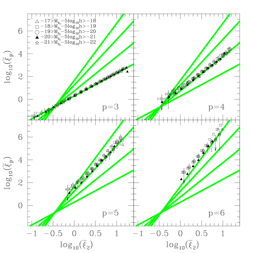
Figure 5: The volume averaged correlation functions, $\bar{\xi}_{p}$, for $p=3$ to $6$, plotted as a function of the variance, $\bar{\xi}_{2}$. Each panel corresponds to a different order plotted on the ordinate, as indicated by the legend. (Note that $\bar{\xi}_{5}$ and $\bar{\xi}_{6}$ are not plotted for the brightest sample, as they are too noisy.) The symbols refer to different magnitude ranges as given by the key in the first panel. The line styles denote the results for different absolute magnitude ranges, as indicated by legend. The thick grey lines show power-laws with slopes of $2$, $3$, $4$ and $5$ in order of increasing amplitude, which are intended to act as a reference.

We use the measured volume averaged correlation functions from Fig. 3 to test the hierarchical clustering model set out in Section 2.2 and Eq. 7. In Fig. 5, we plot the $p=3$–$6$ point volume averaged correlation functions as a function of the variance (or two-point function) measured on the same scale. Small values of the moments correspond to large cells. The thick grey lines show the higher order moments expected in the hierarchical model. (From Eq. 7, the offsets of these lines are the hierarchical amplitudes $S_{p}$. We have used the best fit values of $S_{p}$ that we obtain later on in this Section. However, the width of the lines does not indicate the error on the fit: the lines are intended merely to guide the eye.) On small scales (large variances), hierarchical scaling is followed. On intermediate and large scales, for which the variance drops below $\sim 1.3$, the measured moments depart somewhat from the hierarchical scaling behaviour, particularly in the case of the higher orders.

Figure 6: The hierarchical amplitudes, $S_{p}$, for $p=3,4$ and $5$, plotted as a function of cell radius for the galaxy samples defined in Table 1. Each panel shows the results for a different volume limited catalogue, as indicated by the legend. The points with errorbars show the results obtained from the full volume limited samples: triangles show $S_{3}$, squares show $S_{4}$ and pentagons show $S_{5}$. The solid lines show the best fit values and the dotted lines indicate the $1\sigma$ errors on the fits, as described in the text. The lines are plotted over the range of scales used in the fits.

The hierarchical scaling of the higher order correlation functions is exploited to plot the hierarchical amplitudes $S_{p}=\bar{\xi}_{p}/\bar{\xi}_{2}^{p-1}$ as a function of cell radius in Fig. 6. Each panel corresponds to a different volume limited sample, where the lines and points correspond to $S_{3}$, $S_{4}$ and $S_{5}$ in order of increasing amplitude. The hierarchical amplitudes measured from the two brightest volume limited samples systematically show an increase around $10h^{-1}$Mpc. This effect is particularly significant in the $-19>M_{b_{\rm J}}-5\log_{10}h>-20$ sample, with the $S_{p}$ increasing by a factor of 2 to 5 depending on $p$. On smaller scales the hierarchical amplitudes are essentially independent of the cell radius for all magnitude ranges considered. It should be noted that the $S_{p}$ measured in real space vary more strongly in amplitude with scale than in redshift space, particularly at small cell radii (Gaztañaga 1994; Szapudi et al. 1995, Szapudi & Gaztañaga 1998).

We have fit constant values to the measured $S_{p}$, using the principal component analysis outlined in Section 3.3. This approach takes into account the correlations between the measurements on different scales. The range of scales used to fit $S_{p}$ is held fixed for each volume limited sample and is quoted in Table 2. Typically, there are ten values of $S_{p}$ in the range considered in the fits. The principal component analysis reveals that just $2-4$ linear combinations of these points account for more than $90$% of the variance; this gives a fairer impression of the number of independent data points. The principal eigenvector is in all cases almost independent of scale, i.e. its effect is to move all the points coherently up and down (driven by large scale variation in the mean density estimated from the survey). Therefore, the best fitting constant tends to favour a fit either slightly above or below each set of data points. This is exactly what is seen in the various panels of Fig. 6. The best fit constants to the measured $S_{p}$ are given in Table 2, along with an error from the principal component analysis. The fits to $S_{3}$ and $S_{4}$ for the $-19>M_{b_{\rm J}}-5\log_{10}h>-20$ sample are poor in terms of the reduced $\chi^{2}$. There some dependence of the $S_{p}$ with increasing luminosity. This behaviour is explored in Section 5.

4.3 Systematic effects: the influence of superclusters

The higher order moments of the CPDF are sensitive to the presence of massive structures that contribute to the extreme event tail of the count distribution. It is therefore important to examine the 2dFGRS to look for any rare large scale structures that could exert a significant influence on the form of the CPDF. The projected density of galaxies in the right ascension-redshift plane for a volume limited catalogue defined by the magnitude range $-19>M_{b_{\rm J}}-5\log_{10}h>-20$ is plotted in figure 1 of Baugh et al. (2004). There are two clear hot spots or superstructures apparent in this figure, one in the NGP at a redshift of $z=0.08$ and a right ascension of 3.4 hours, and the other in the SGP at $z=0.11$ at a right ascension of $0.2$ hours. These structures are confirmed as superclusters of galaxies in the group catalogue constructed from the flux limited 2dFGRS (Eke et al. 2004); of the 94 groups in the full flux limited survey out to $z\sim 0.15$ with 9 or more members and estimated masses above $5\times 10^{14}h^{-1}M_{\odot}$, 20% reside in these superclusters. As a result of the redshift at which these superclusters lie, these structures are only influential in volume limited samples brighter than $M_{b_{\rm J}}-5\log_{10}h=-18$.

The results presented earlier in this Section show features that could be due to the presence of these superclusters. For example, the volume averaged correlation functions for the $-19>M_{b_{\rm J}}-5\log_{10}h>-20$ sample plotted in Fig. 3 appear to have more power on large scales than those measured from the other volume limited samples. This is consistent with the theoretical expectations for measurements that are strongly affected by the presence of a supercluster: a boost in the clustering amplitude on large scales, due to a structure with a larger bias, and a reduction in the clustering amplitude on small scales arising from the large velocity dispersions within the clusters making up the structure.

To investigate this hypothesis, we have carried out the test of removing the two superclusters from the sample and recomputing the volume averaged correlation functions. The goal of this exercise is not to “correct” the measured correlation functions but rather to illustrate the impact of the superclusters on our results. We remove the superclusters by masking out their central densest regions, corresponding to prohibiting the placement of cells within a sphere of radius $25h^{-1}$Mpc from each supercluster centre (for a different approach on how to take this type of effect into account see Colombi, Bouchet & Schaeffer 1994 and Fry & Gaztañaga 1994).

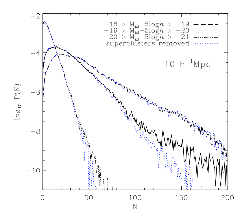
Figure 7: The probability, $P_{N}$, of finding exactly $N$ galaxies in randomly placed cells of radius $10h^{-1}$Mpc (the CPDF, Eq. 2), for different volume limited galaxy samples. Each bold line shows the full volume CPDF, while the individual dotted lines give the result after the supercluster regions have been omitted from the analysis, as described in Section 4.3.

Fig. 7 shows the effect of the supercluster removal on the tail of the CPDF for $10h^{-1}$Mpc radius cells, calculated for three volume limited catalogues centred on $L^{*}$. The mean number of galaxies in a cell for each galaxy sample is roughly $40$, $24$, and $6$ going from faintest to brightest. The presence of the two superclusters makes a clear difference to the high $N$ counts for galaxy samples brighter than $M_{b_{\rm J}}-5\log_{10}h=-19$. The maximum redshift of the faint volume limited catalogue in this figure only marginally includes the NGP supercluster, and so $P_{N}$ remains essentially unaffected in this case.

Fig. 8 shows volume averaged correlation functions of order $p=2,3,4$ for three volume limited catalogues from Table 1, where each panel corresponds to a fixed absolute magnitude range. The lines correspond to different orders of clustering, starting with the lowest in amplitude, the two point volume averaged correlation function, and moving through to the four point function, at which we stop plotting the results for clarity although the trends shown continue up to sixth order. The solid curves show the correlation functions measured from the full volume limited samples, as shown previously in Fig. 6, and the dashed lines show the results when the regions containing the superclusters are excluded from the CPDF. The higher order correlation functions are systematically boosted on intermediate and large scales when the superclusters are included in the analysis. The precise scale on which the correlation functions become sensitive to the presence of the superclusters depends upon the order; for the four point function, the two estimates of the correlation function typically deviate for cells of radius $3h^{-1}$Mpc and larger.

Figure 8: The volume averaged correlation functions for $p=2$ to $4$, with each panel showing the results from a different volume limited sample, as indicated by the legend. The solid lines show the estimates from the full volumes and the dashed lines show the results when the supercluster regions are omitted from the analysis. For clarity, errorbars are only plotted on the solid curves for order $p=4$.

Figure 9: The hierarchical amplitudes, $S_{3}$ (triangles), $S_{4}$ (squares) and $S_{5}$ (pentagons). The top panel corresponds to galaxies with $-19>M_{b_{\rm J}}-5\log_{10}h>-20$ and the bottom panel to $-20>M_{b_{\rm J}}-5\log_{10}h>-21$. The open symbols with errorbars show the results obtained using the full volume limited catalogues. The filled symbols show how the results change when regions containing the two superclusters are omitted from the analysis.

The impact on the hierarchical amplitudes, $S_{p}$, of removing the superclusters in shown in Fig. 9, in which we plot the results for the volume limited sample defined by $-19>M_{b_{\rm J}}-5\log_{10}h>-20$. In Fig. 9, the open points show the hierarchical amplitudes measured from the full volume limited sample. The filled symbols show the results obtained from the same volume but with the supercluster regions masked out. The $S_{p}$ obtained when the two superclusters are removed from the analysis are much closer to being independent of cell size. The sensitivity of higher orders to rare peaks has been noticed in earlier analyses of galaxy surveys (Groth & Peebles 1977; Gaztañaga 1992; Bouchet et al. 1993; Lahav et al. 1993; ; Gaztañaga 1994; Hoyle et al. 2000).

5 Interpretation and the implications for galaxy bias

In this Section we quantify how the hierarchical amplitudes scale with galaxy luminosity and discuss the implications of our results for simple models of galaxy bias. We first test the hypothesis set out in Section 2.4 that the variation in clustering with luminosity apparent in Fig. 3 can be described by a single, relative bias factor, as defined by Eq. 14. The relative bias factors, $b_{r}$, computed from the variance and the deviation from the linear bias model, as quantified by $c_{2}^{\prime}$ (Eq. 17), are listed in Table 2; here the mean value is given by the best $\chi^{2}$ fit over all cell radii. The change in the amplitude of the relative bias with sample luminosity, shown in Fig. 4, is in excellent agreement with the trend found by Norberg et al. (2001), who analysed the projected spatial clustering of 2dFGRS galaxies. This agreement is remarkable given the different approaches used to measure the two-point correlations and the fact that the analysis in this paper is in redshift space, whereas the study carried out by Norberg et al. was unaffected by peculiar motions.

The coefficients $c_{2}^{\prime}$ are different from zero at a 1-$\sigma$ level. These findings are consistent with a small deviation from the linear biasing model (at a 2-sigma level for the brighter samples). This is in qualitative agreement with the estimation of $c_{2}$ using the the bispectrum (Scoccimarro 2000, Verde et al. 2002) or the 3-point function measured from the parent APM galaxy survey (Frieman & Gaztañaga 1999).

Figure 10: The variation of the hierarchical amplitudes, $S_{p}$, with absolute magnitude. The points are plotted at the median magnitude of each volume limited sample and the horizontal bars indicate the interval in which $25\%$ to $75\%$ of the galaxies fall, computed using the 2dFGRS luminosity function fit quoted by Norberg et al. (2002b). Each panel shows the results for a different order of clustering. The dotted line shows predictions of the linear relative bias model for the variation of the $S_{p}$ with luminosity (Eq. 15). The solid lines show linear fits in log luminosity to the observed trend in the value of $S_{p}$ with sample luminosity (see text of Section $5$ for details).

The variation of the hierarchical amplitudes with luminosity is plotted in Fig. 10. Each panel corresponds to a different order $p$. The filled points show the hierarchical amplitudes averaged over the different cell radii employed (these values and the associated errors are given in Table 2). The dotted line shows the hierarchical amplitudes predicted by the linear relative bias model (Eq. 15), using the best fit bias factors stated in Table 2. This model gives a rough approximation to the data. However, the observed variation of $S_{p}$ with luminosity is somewhat better described by a linear fit in the logarithm of luminosity, as shown by the solid lines. This implies that the dependence of the hierarchical amplitudes on luminosity is more complicated than expected in the simple relative bias model of Eq. 15 (as does the fact that we find some evidence for non-zero values for $c_{2}^{\prime}$). The solid lines show the best linear fit to the hierarchical amplitudes as a function of the logarithm of the median luminosity of the samples:

$$S^{G}_{p}=A_{p}+B_{p}\log_{10}\left(\frac{L}{L_{*}}\right).$$ (18)

We find a greater than $2-\sigma$ ($\Delta\chi^{2}>7.2$ for two parameters) detection of a non-zero value for $B_{3}$. However, for $p>3$, the constraints on $B_{p}$ are much weaker and there is no clear evidence for a luminosity dependence in the $S_{p}$ values in these cases. For completeness, the best fit values for each order are: $(A_{3},B_{3})=(2.07,-0.40)$, $(A_{4},B_{4})=(6.15,-2.51)$, $(A_{5},B_{5})=(21.3,-13.5)$, $(A_{6},B_{6})=(58,-39)$.

6 Conclusions

In this paper we have measured the higher order correlation functions of galaxies in volume limited samples drawn from the 2dFGRS. The most recent comparable work is the analysis of the Stromlo-APM and UKST redshift surveys by Hoyle, Szapudi & Baugh (2000). These authors also considered volume limited subsamples drawn from the flux limited redshift survey. The largest UKST sample considered by Hoyle et al. contained 500 galaxies and covered a volume of $9\times 10^{5}h^{-3}{\rm Mpc}^{3}$; the reference sample used in our work contains 90 times this number of galaxies and covers ten times the volume. In our analysis, we can follow the variation of clustering over more than a decade in luminosity, whereas Hoyle et al. had to focus their attention around $L_{*}$.

The measurement of the higher order galaxy correlation functions is still challenging, however. In spite of the order of magnitude increase in size that the 2dFGRS represents over previously completed surveys, we have found that the higher order moments that we measure are somewhat sensitive to the presence of large structures. In particular, there are two superclusters that influence our measurements, one in the SGP region and the other in the NGP. These structures contain a sizeable fraction of the cluster mass groups in the 2dFGRS (Eke et al. 2004). The inclusion of these structures has an impact on our estimates of the three point and higher order volume averaged correlation functions on scales around $4-10h^{-1}$Mpc and above, depending on the order of the correlation function. For this reason, we have presented measurements of the higher order correlation functions both with and without these structures. We stress that the removal of these superclusters should not be considered a correction to the full catalogue results, but rather as an indication of the impact of rare structures on our results for the higher order moments. On the other hand, the up-turn that we find in the values of the hierarchical amplitudes on large scales is predicted by some structure formation models; for example models with non-Gaussian initial density fields predict a similar form for the $S_{p}$ as we measure from the full volume limited samples (Gaztañaga & Mähönen 1996; Gaztañaga & Fosalba 1998; Bernardeau et al. 2002).

The difficulties in estimating $S_{p}$ values on large, quasi-linear scales ($>10h^{-1}$Mpc), prevent a direct comparison with perturbation theory (see Bernardeau et al. 2002). The current best estimates on these scales are still those measured from the angular APM Galaxy Survey (Gaztañaga 1994, Szapudi et al. 1995, Szapudi & Gaztañaga 1998). At the time of writing, the results from the SDSS Early Data Release are still limited to small scales (Gaztañaga 2002, Szapudi et al. 2002). Despite being unable to make a robust measurement of the higher order correlation functions on the very large scales for which weakly non-linear perturbation theory is applicable, we are still able to reach a number of interesting conclusions:

• We have demonstrated that the higher order galaxy correlation functions measured from the 2dFGRS follow a hierarchical scaling. Baugh et al. (2004) showed that $L_{*}$ galaxies display higher order correlation functions that scale in a hierarchical fashion; we have extended these authors’ analysis to cover a wide range of galaxy luminosity. The higher order moments of the galaxy count distribution are proportional to the variance raised to a power that depends upon the order of the correlation function under consideration. This behaviour holds on physical scales ranging from those on which we expect the underlying density fluctuations to be strongly nonlinear all the way through to quasi-linear scales. This scaling has been tested up to the six point correlation function for the first time using a redshift survey. This confirms the conclusions of a complementary analysis carried out by Croton et al. (2004), who found hierarchical scaling when measuring the reduced void probability function of the 2dFGRS.

• We have estimated values of the hierarchical amplitudes, $S_{p}=\bar{\xi}_{p}/\bar{\xi}^{p-1}_{2}$, for cells of different radii. The hierarchical amplitudes are approximately constant on small to medium scales (depending on the order considered), while for the larger volumes, $S_{p}$ seem to increase with radius at large scales. Although this could in principle result from a boundary or mask effect (e.g. see Szapudi & Gaztañaga 1998; Bernardeau et al. 2002), we have shown with mock catalogues that this is not the case here (e.g. see Fig. 1). If the two most massive superclusters in the survey are removed from the analysis, the hierarchical amplitudes are remarkably independent over all scales. That the $S_{p}$ are roughly constant on small scales, with smaller amplitudes than in real space (e.g. Gaztañaga 1994), has been noted before for measurements in redshift space. It arises due to a cancellation of the enhanced signal on small scales in real space by a damping of clustering in redshift space due to peculiar motions (Lahav et al. 1993; Fry & Gaztañaga 1994; Hivon et al. 1995; Hoyle et al. 2000; Bernardeau et al. 2002).

• We find that the amplitude of the higher order correlation functions scales with luminosity. The magnitude of the luminosity segregation increases with the order of the correlation (see Fig. 4). For the variance, $\bar{\xi}_{2}$, the strength of the trend is in very good agreement with that reported by Norberg et al. (2001), but note that these authors measured the luminosity segregation in real space, whereas our results are in redshift space. The strength of the luminosity segregation for higher orders can be mostly explained as the result of hierarchical scaling $\bar{\xi}_{p}\sim\bar{\xi}_{2}^{p-1}$, so that most of the effect can be attributed to luminosity segregation in the variance. This can be seen in Fig. 5 where data from different luminosities trace out the same hierarchical curve with little scatter.

• We find some evidence for a residual dependence of $S_{p}$ on luminosity, although the effect is only significant within the errors for the skewness $p=3$ (greater than $2\sigma$ level). It is not clear whether this is driven by a pure luminosity dependence of the higher order clustering or by a change in the galaxy mix with luminosity, with different galaxy types having different $S_{p}$ or by a combination of the two effects: see Norberg et al. (2002a) for an investigation of this point for the 2-point correlation function. A simple linear relative bias model (dotted line in Fig. 10) does not reproduce the dependence of the $S_{p}$ on luminosity.

We have interpreted our results in terms of a simple, local bias model, and we have quantified trends in clustering amplitude with luminosity by estimating relative bias factors. These measurements, summarised in Table 2, extend the constraints upon models of galaxy formation derived from the two-point correlation function, quantifying the shape of the tails of the count probability distribution as well as its width.

References

- [Baugh, Gaztañaga & Efstathiou (1995)] Baugh C.M., Gaztañaga E., Efstathiou G., 1995, MNRAS, 274, 1049.
- [spinoff] Baugh C.M., et al., (the 2dFGRS team), 2004, submitted to MNRAS. astro-ph/0401405
- [Berlind et al. (2003)] Berlind A. A., Weinberg D. H., Benson A.J., Baugh C. M., Cole S., Davé R., Frenk C.S., Jenkins A., Katz N., Lacey C.G., 2003, ApJ, 593, 1.
- [Benson et al. (2000)] Benson A.J., Cole S., Frenk C.S., Baugh C.M., Lacey C.G., 2000, MNRAS, 311, 793.
- [Bernardeau (1994)] Bernardeau F., 1994, Astron. & Astroph., 291, 697.
- [Bernardeau et al. 2002] Bernardeau F., Colombi S., Gaztañaga E., Scoccimarro R., 2002, Phys. Rep., 367, 1
- [Bernstein (1994)] Bernstein G.M., 1994, ApJ, 424, 569.
- [Bouchet et al. (1993)] Bouchet F.R., Strauss M.A., Davis M., Fisher K.B., Yahil A., Huchra J.P., 1993, ApJ, 417, 36.
- [Cole, Hatton, Weinberg, & Frenk(1998)] Cole S., Hatton S., Weinberg D. H., & Frenk C. S. 1998, MNRAS, 300, 945
- [Cole] Cole S. & Kaiser N., 1989, MNRAS, 237, 1127.
- [Colombi, Bouchet, & Schaeffer(1994)] Colombi S., Bouchet F. R., & Schaeffer R. 1994, A&A, 281, 301
- [Colless et al.(2001)] Colless M., et al. (the 2dFGRS Team), 2001, MNRAS, 328, 1039
- [Colless et al.(2003)] Colless M., et al. (the 2dFGRS Team), 2003, astro-ph/0306581
- [Croton et al.(2004)] Croton D. et al. (the 2dFGRS Team), 2004, astro-ph/0401406.
- [Efstathiou et al.(1990)] Efstathiou G., Kaiser N., Saunders W., Lawrence A., Rowan-Robinson M., Ellis R.S., Frenk C.S., 1990, MNRAS, 247, 10P
- [Eke et al.(2004)] Eke V.R., et al. (the 2dFGRS Team), 2004, MNRAS, in press (astro-ph/0401XXX).
- [Evrard] Evrard A.E., et al. (the Virgo Consortium), 2002, ApJ, 573, 7.
- [Feldman Scoccimarro et al. (2001)] Feldman, H.A, Frieman, J.A., Fry, J.N., Scoccimarro R., 2001, Phys. Rev. Lett. 86 1434.
- [Fosalba & Gaztañaga (1998)] Fosalba P., Gaztañaga E., 1998, MNRAS, 301, 503.
- [Frieman & Gaztañaga(1999)] Frieman J.A. & Gaztañaga E., 1999, ApJ, 521, L83
- [Fry & Gaztañaga(1993)] Fry J. N. & Gaztañaga E., 1993, ApJ, 413, 447
- [Fry & Gaztañaga(1994)] Fry J. N. & Gaztañaga E., 1994, ApJ, 425, 1
- [Gaztañaga(1992)] Gaztañaga E., 1992, ApJ, 398, L17
- [Gaztañaga(1994)] Gaztañaga E., 1994, MNRAS, 268, 913
- [Gaztañaga(2002)] Gaztañaga E., 2002, ApJ, 580, 144
- [Gaztañaga & Bern (1998)] Gaztañaga E. & Bernardeau F., 1998, A.& A., 331, 829
- [Gaztañaga & Yokoyama(1993)] Gaztañaga E. & Yokoyama J., 1993, ApJ, 403, 450
- [Gaztañaga & Baugh (1995)] Gaztañaga E., Baugh C.M., 1995, MNRAS, 273, L1.
- [Gaztañaga & Mahonen (1996)] Gaztañaga E., Mahonen P., 1996, ApJ, 462, L1.
- [Gaztañaga & Fosalba (1998)] Gaztañaga E., Fosalba P., 1998, MNRAS, 301, 524.
- [Gaztañaga & Juszkiewicz (2001)] Gaztañaga E., Juszkiewicz R., 2001, ApJ, 558, L1.
- [Gaztañaga & Wagg (2003)] Gaztañaga E., Wagg J., 2003, Phys.Rev.D, 68, 21302.
- [Ghigna et al. (1996)] Ghigna S., Bonometto S.A., Guzzo L., Giovanello R., Haynes M.P., Klypin A. & Primack J.R., 1996, ApJ, 463, 395
- [Gia] Porciani C., Giavalisco M., 2002, ApJ, 565, 24.
- [] Groth E.J., Peebles, P.J.E., 1977, ApJ, 217, 385.
- [Hawkins et al. (2003)] Hawkins E., et al. (the 2dFGRS Team), 2003, MNRAS, 346, 78. (astro-ph/0212375)
- [Hinshaw et al. (2003)] Hinshaw G., et al. (the WMAP Team), 2003, ApJS, 148, 135. (astro-ph/0302217)
- [Hivon et al. (1995)] Hivon E., Bouchet F.R., Colombi S., Juszkiewicz R., 1995, Astron. & Astroph., 298, 643.
- [Hoyle, Szapudi, & Baugh(2000)] Hoyle F., Szapudi I., & Baugh C. M., 2000, MNRAS, 317, L51
- [Hui & Gaztañaga(1999)] Hui L. & Gaztañaga E., 1999, ApJ, 519, 622
- [Juszkiewicz et al. (1993)] Juszkiewicz R., Bouchet F.R., Colombi S., 1993, ApJ, 412, L9.
- [Kamionkowski & Kowsowsky (1999)] Kamionkowski M., Kowsowsky A., 1999, Ann. Rev. Nuclear & Particle Science, 49, 77.
- [Komatsu et al. 2003] Komatsu, E., et al. 2003, ApJS, 148, 119
- [Kauffmann et al (1999)] Kauffmann G., Colberg J.M., Diaferio A., White S.D.M., 1999, MNRAS, 303, 188.
- [Kuo et al (2004)] Kuo C. L., et al. (the ACBAR Team), 2004, ApJ, 600, 32. (astro-ph/0212289)
- [Lahav, Itoh, Inagaki, & Suto(1993)] Lahav O., Itoh M., Inagaki S., & Suto Y., 1993, ApJ, 402, 387
- [Lahav et al. (2002)] Lahav O., et al. (the 2dFGRS Team), 2002, MNRAS, 333, 961.
- [Maddox et al. (1990)] Maddox S. J., Efstathiou G., Sutherland W. J. & Sutherland W.J., 1990, MNRAS, 246, 433
- [Maddox, Efstathiou, & Sutherland(1996)] Maddox S. J., Efstathiou G., & Sutherland W. J., 1996, MNRAS, 283, 1227.
- [Mason et al. 2003] Mason B.S., et al. (the CBI Team), 2003, ApJ, 591, 540.
- [Mason et al. 2003] Mo H.J., Jing Y.P., White S.D.M., 1997, MNRAS, 284, 189
- [] Mo H.J. & White S.D.M., 1996, MNRAS, 282, 347.
- [Netterfield et al.(2002)] Netterfield C.B., et al. (the BOOMERANG Team), 2002, ApJ, 571, 604.
- [Norberg et al.(2001)] Norberg P., et al. (the 2dFGRS Team), 2001, MNRAS, 328, 64
- [Norberg et al.(2002a)] Norberg P., et al. (the 2dFGRS Team), 2002a, MNRAS, 332, 827
- [Norberg et al.(2002b)] Norberg P., et al. (the 2dFGRS Team), 2002b, MNRAS, 336, 907
- [Padilla & Baugh (2002)] Padilla N.D., Baugh C.M., 2003, MNRAS, 343, 796.
- [Peebles(1980)] Peebles P. J. E., 1980, The Large-Scale Structure of the Universe (Princeton Univ Press)
- [Percival] Percival W., et al. (the 2dFGRS team), 2001, MNRAS, 327, 1297.
- [Scoccimarro et al. (2000)] Scoccimarro R., 2000, ApJ, 544, 597.
- [Scoccimarro et al. (2001)] Scoccimarro R., Sheth R., Hui L., Jain B., 2001, ApJ, 546, 20.
- [Scoccimarro et al. (2003)] Scoccimarro R., Sefusatti E., Zaldarriaga, M., 2003, astro-ph/0312286.
- [Scott et al. (2003)] Scott P.F., et al. (the VSA Team), 2003, MNRAS, 341, 1076.
- [Szapudi et al. (1995)] Szapudi I., Dalton G.B., Efstathiou G., Szalay A.S., 1995, ApJ, 444, 520.
- [Szapudi & Gazta (1998)] Szapudi I., & Gaztañaga E., 1998, MNRAS, 300, 493.
- [Szapudi et al. (1999)] Szapudi I., Quinn T., Stadel J., Lake G., 1999, ApJ, 517, 54.
- [Szapudi et al. (2000)] Szapudi I., Branchini E., Frenk C.S., Maddox S., Saunders W., 2000, MNRAS, 318, L45.
- [Szapudi et al. (2002)] Szapudi et al. (the SDSS collaboration) 2002, ApJ, 570, 75
- [Tegmark] Tegmark M., et al. (the SDSS collaboration), 2004, ApJ, submitted. astro-ph/0310725
- [Verde et al.(2002)] Verde L., et al. (the 2dFGRS Team), 2002, MNRAS, 335, 432
- [White (1979)] White S.D.M., 1979, MNRAS, 186, 145.
- [York et al.(2000)] York D.G., et al. (the SDSS Team), 2000, AJ, 120, 1579.
- [Zehavi et al.(2002)] Zehavi I., et al. (the SDSS Team), 2002, ApJ, 571, 172