Hot Interstellar Gas and Stellar Energy Feedback in the Antennae Galaxies

Abstract

We have analyzed $Chandra$ archival observations of the Antennae galaxies to study the distribution and physical properties of its hot interstellar gas. Eleven distinct diffuse X-ray emission regions are selected according to their underlying interstellar structures and star formation activity. The X-ray spectra of these regions are used to determine their thermal energy contents and cooling timescales. Young star clusters in these regions are also identified and their photometric measurements are compared to evolutionary stellar population synthesis models to assess their masses and ages. The cluster properties are then used to determine the stellar wind and supernova energies injected into the ISM. Comparisons between the thermal energy in the hot ISM and the expected stellar energy input show that young star clusters are sufficient to power the X-ray-emitting gas in some, but not all, active star formation regions. Super-star clusters, with masses $\geq 1\times 10^{5}$ M_⊙, heat the ISM, but the yield of hot interstellar gas is not directly proportional to the cluster mass. Finally, there exist diffuse X-ray emission regions which do not show active star formation or massive young star clusters. These regions may be powered by field stars or low-mass clusters formed within the last $\sim$100 Myr.

1 Introduction

The interacting galaxies NGC 4038/4039, nicknamed “The Antennae” galaxies, are the nearest example of a major merger of two massive disk galaxies and provide an excellent opportunity to study galaxy collisions in detail. The Antennae are located at a distance of only 19.2 Mpc (for H₀= 75 km s^-1 Mpc^-1), allowing a detailed examination of astrophysical processes with high resolution at multiple wavelengths (Whitmore et al., 1999; Zhang et al., 2001).

The gravitational interactions from the merger trigger star formation and produce conditions appropriate for globular clusters to form. Thus, the Antennae contain many sites of active star formation, giant H II regions, and young super-star clusters. Massive stars interact with the interstellar medium (ISM) via fast stellar winds and supernova ejecta. These dynamic interactions produce hot ($\geq 10^{6}$ K) ionized gas which can be studied in X-rays. Examining the characteristics of the X-ray emission from the Antennae galaxies is important in determining how the hot interstellar gas is energized and distributed. This will allow us to study stellar energy feedback processes in different types of star formation regions, especially in young globular clusters, i.e., young super-star clusters, which are not available in our Galaxy or nearby Local Group galaxies.

Many X-ray telescopes have observed the Antennae galaxies. The Einstein observations were the first to show diffuse X-ray emission, but were unable to resolve the point sources from the diffuse emission (Fabbiano et al., 1982; Fabbiano & Trinchieri, 1983). Subsequent observations with ROSAT PSPC, which had higher spatial and spectral resolution, showed 55% of the X-ray flux (in the PSPC band of 0.1-2.4 keV) from the Antennae to be resolved into discrete sources with the rest predominantly diffuse emission (Read et al., 1995). ROSAT HRI observations were able to resolve twelve discrete sources (Fabbiano et al., 1997). ASCA observations confirmed a hard X-ray component and softer gaseous emission (Read et al., 1995; Sansom et al., 1996). The advent of the Chandra X-ray Observatory finally made it possible to clearly resolve point sources from diffuse emission. Using Chandra ACIS-S observations, 48 point X-ray sources are detected in the Antennae galaxies; these point sources contribute 81% of the emission in the 2.0–10.0 keV band but only 32% of the emission in the 0.1–2.0 keV band (Fabbiano et al., 2001). The discrete sources in the Antennae have diverse spectral properties, with the most luminous ones showing hard emission consistent with X-ray binaries and the faintest ones displaying softer emission similar to supernova remnants (SNRs) or hot ISM (Zezas et al., 2002a). Many X-ray sources show good correspondence with the young stellar clusters (Zezas et al., 2002b).

Chandra observations of the Antennae galaxies vividly portray a dynamic ISM with wide-spread hot gas throughout both galaxies (Fabbiano et al., 2001). The active star cluster formation that is responsible for the large H II complexes, such as giant H II regions and supergiant shells, must also contribute to the production of hot ISM. Previous investigations of hot gas in the Antennae did not take into account the physical association with the young stellar clusters (e.g., Fabbiano et al., 2003). Therefore, we have compared the distribution of diffuse X-ray emission with the underlying star cluster content and cooler interstellar structures revealed in optical images, identified physical associations between them, and analyzed the physical properties of the hot interstellar gas accordingly. We have further used the photometry of the underlying clusters (Whitmore et al., 1999) to determine their ages and masses in order to derive the expected stellar wind and supernova energies injected into the ISM. These results allow us to compare the thermal energy stored in the hot X-ray-emitting medium to the stellar energy input and compare the cooling timescale of the hot gas to the age of the clusters so that we may assess the role of the young clusters in energizing the ISM.

In this paper, we describe the Chandra observations and complementary Hubble Space Telescope images and ground-based echelle observations in §2, report the identification of distinct interstellar diffuse X-ray sources in §3, and analyze physical properties of the hot, X-ray-emitting ISM in §4. We consider the stellar energy feedback from the clusters and compare it to the thermal energy stored in the hot ISM in §5, and discuss the production of hot ISM with and without super-star clusters in §6. A summary is given in §7.

2 Observations and Reduction

The Antennae galaxies were observed with the back-illuminated CCD chip S3 of the ACIS-S array onboard the Chandra X-Ray Observatory on 1999 December 1 for a total exposure time of 72.5 ks (Observation ID: 315; PI: Murray), on 2001 December 29 for 69.9 ks (Observation ID: 3040; PI: Fabbiano), and on 2002 April 18 for 68.0 ks (Observation ID: 3043; PI: Fabbiano). We retrieved level 1 and level 2 processed data from the Chandra Data Center. The data reduction and analysis were performed using the Chandra X-Ray Center software CIAO v2.2.1 and HEASARC FTOOLS and XSPEC v11.0.1 routines (Arnaud, 1996). The latter two observations were affected by high background for 11.8 ks and 14.6 ks, respectively; these high-background periods were excluded in our analysis. The three observations were merged to increase the signal-to-noise ratio for the analysis of the spatial distribution and spectral properties of the X-ray emission. The spectral analysis was carried out by computing the calibration files for the individual observations and averaging them using weights proportional to their net exposure times.

To associate the X-ray emission of the Antennae galaxies to the cooler ionized ISM and the underlying stellar content, we have also retrieved archival Hubble Space Telescope images taken with the Wide Field and Planetary Camera 2 (WFPC2) in the F555W and F658N filters. The F555W image, similar to a $V$-band image, has a total exposure of 4,400 s and shows the star clusters. The F658N filter, originally designed as an [N II] filter, contains the red-shifted H$\alpha$ line over the velocity range covered by the Antennae galaxies. Thus, the F658N image of the Antennae is essentially an H$\alpha$ image contaminated only by the weak [N II] $\lambda$6548 line, and should show the 10⁴ K ionized ISM well.

To study the dynamics of a supergiant shell and three giant H II regions with bright X-ray emission, we obtained high-dispersion spectroscopic observations with the echelle spectrograph on the Blanco 4m telescope at the Cerro Tololo Inter-American Observatory on 2002 March 24 and 25. For these observations, a 79 line mm^-1 echelle grating was used. The spectrograph was configured in a long-slit, single-order mode by replacing the cross-disperser by a flat mirror and inserting a post-slit broad H$\alpha$ filter (central wavelength 6563 Å with 75 Å FWHM). The long-focus red camera was used to obtain a reciprocal dispersion of 3.5 Å mm^-1 at H$\alpha$. The SITe2K #5 CCD detector with 24 $\mu$m pixel size was read out with a 2-pixel binning in the spatial direction, providing a spatial sampling of 0$\farcs$53 pixel^-1 along the slit and a spectral sampling of $\sim$0.08 Å pixel^-1 along the dispersion axis.

A 1$\farcs$5 wide slit was used in the echelle observations. A total of four long-slit observations were obtained with 1,200 sec integration time each. Two of the observations were centered at a single position, $\alpha$(J2000)$=$12^h01^m51.^s3, $\delta$(J2000)$=$$-$18^∘51′47″, with the slit oriented in the east-west direction. The other two observations were made with the slit oriented in the north-south direction centered at the positions: $\alpha$(J2000)$=$12^h01^m50.^s3, $\delta$(J2000)$=$$-$18^∘52′14″, and $\alpha$(J2000)$=$12^h01^m50.^s6, $\delta$(J2000)$=$$-$18^∘52′14″. These three slit positions will be called S1, S2, and S3, respectively. The echelle observations were reduced using standard packages in IRAF. All spectra were bias and dark corrected, and cosmic-ray events were removed by hand. Observations of a Th–Ar lamp were used to determine the dispersion correction and then telluric lines in the source observations were used to check the absolute wavelength calibration. The resultant spectra had an instrumental resolution of 0.26 Å (12 km s^-1 at H$\alpha$), as measured by the FWHM of the unresolved telluric emission lines.

3 Interstellar Sources of X-ray Emission from the Antennae

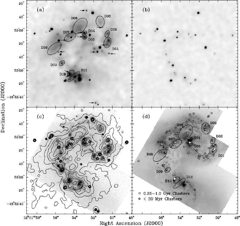
Figure 1: The top two panels contain adaptively smoothed X-ray images of the Antennae galaxies in the 0.3–2.0 keV energy band (top left) and 2.5–6.0 keV energy band (top right). See the text for details of this merged X-ray image. The pixel size is 0$\farcs$492 and the maximum smoothing scale is 2″. The locations of the 11 elliptical regions that have been selected for study are shown in the soft energy image. The positions of soft point sources that are possibly SNR candidates are marked by arrows in the soft band image. The bottom left panel presents an HST WFPC2 H$\alpha$ image (F658N) overlaid by X-ray contours for the 0.3–2.0 keV band. The contour levels are 0.2, 0.45, 0.8, 1.2, 1.8, 2.5, 4.5, 10, 40, and 150 counts pixel^-1. The bottom right panel displays an HST WFPC2 $V$-band (F555W) image with the locations of clusters and the 11 diffuse X-ray emission regions marked.

The X-ray emission from the Antennae galaxies has a complex morphology, consisting of both point sources and diffuse emission. To search for X-ray emission from the hot interstellar gas, we have made adaptively smoothed images of the Antennae in the soft (0.3–2.0 keV) and hard (2.5–6.0 keV) bands and present these images in Figures 1a and 1b. Comparisons between these two images show that the diffuse emission is soft and some small, discrete sources are also soft. The diffuse soft X-ray emission most likely originates from the hot ($>$ $10^{6}$ K) ISM. The discrete soft X-ray sources are probably also from the hot ISM and may be unresolved young SNRs. The heating sources of the hot ISM and the progenitors of the supernovae are both likely massive stars.

To examine the relationship between the hot ISM and the massive star formation regions, we have plotted contours showing the soft X-ray emission over the H$\alpha$ image of the Antennae in Figure 1c. A tight correlation is evident between some diffuse X-ray emission and the star forming regions, indicating that the massive stars are indeed responsible for heating the hot ISM. However, there are also extended X-ray emission regions which do not exhibit active star formation. To determine whether this diffuse X-ray emission may be powered by previous star formation activity, we present an HST WFPC2 F555W image in Figure 1d with young (age $<$ 30 Myr) clusters marked by white crosses in filled circles and old (0.25–1.0 Gyr) clusters by open circles. It is clear that bright diffuse X-ray emission is more strongly correlated with the young clusters than the old clusters.

In regions where diffuse X-ray emission is correlated with recent star formation activity, two types of interstellar structures are easily resolved: giant H II regions and supergiant shells. Giant H II regions with sizes of $\geq$ 100 pc are associated with young star formation regions where massive stars with powerful ionizing fluxes are prevalent. Some giant H II regions are located close to the galactic nuclei and may be associated with nuclear starbursts; these will be referred to as circumnuclear starburst regions. Supergiant shells with sizes approaching 1,000 pc have dynamic ages greater than a few $\times 10^{7}$ yr and are associated with older star formation activity. By comparing the physical properties of the hot ISM associated with giant H II regions and supergiant shells, it is possible to study the content and evolution of the hot ISM associated with star formation.

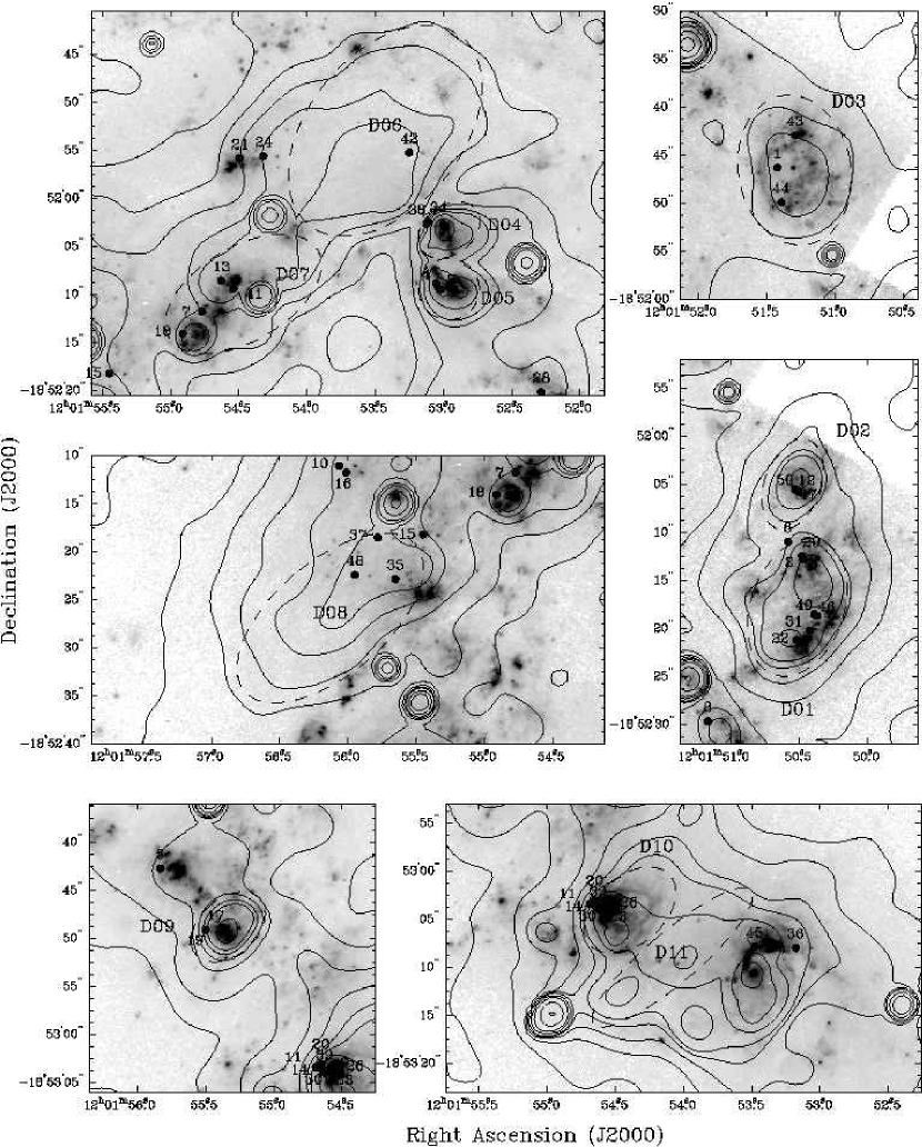
Figure 2: H$\alpha$ images with soft X-ray contours (solid lines) of the 11 diffuse X-ray emission regions that have been chosen for study (black dashed lines). The contour levels are 0.16, 0.35, 0.65, 1.0, 1.45, 1.95, 3.5, 7.0, 30, and 120 counts pixel^-1, and the pixel size is 0$\farcs$492. See Table 1 for regions of point sources that have been excised from our analysis of diffuse X-ray emission. The black dots and numbers represent the location and catalog number of the young star clusters as listed in Table 1 of Whitmore et al. (1999) and in Table 4 of this paper.

We have therefore chosen for detailed analyses diffuse X-ray sources associated with (1) circumnuclear starburst regions, (2) giant H II regions, (3) supergiant shells, and (4) no obvious recent star formation activity. The 11 source regions we have selected are marked in Figure 1a and numbered counterclockwise starting from the west side of the galaxies. Elliptical source apertures are used to extract X-ray fluxes and spectra from these regions. Whenever source regions contain point sources, small regions around the point sources are excised in the analysis of the diffuse X-ray emission. Table 1 lists the positions, major and minor axes, position angles of the major axes, volumes of these source regions, and the total background-subtracted counts detected in the three observations. The volume is calculated assuming an ellipsoidal geometry with the third axis equal to the minor axis of the elliptical region. The excised regions around point sources are given in the notes for Table 1. Figure 2 shows a detailed view of the selected X-ray-emitting regions; in each panel, an H$\alpha$ image is presented with overlays of soft X-ray (0.3–2.0 keV) contours, outlines of the elliptical source apertures, and the identifications of underlying young clusters. Below we describe the 11 source regions, grouped according to their associated star formation activity or interstellar structures.

3.1 Circumnuclear Starburst Regions (D04 and D05)

The nuclei of the two galaxies NGC 4038 and NGC 4039 can be identified from their high CO concentrations (e.g., Liang et al., 2001) or the red color in a true-color image (Whitmore et al., 1999). Both nuclei are associated with active star formation and bright X-ray emission. Due to the presence of bright hard X-ray emission in the nucleus of NGC 4039, we excluded this region from our study. The nucleus of NGC 4038 is bisected by a dust lane, thus two giant H II regions are observed. The H$\alpha$ morphologies of these two giant H II regions are quite different, suggesting that they may be independent from each other and should be examined separately. Therefore, we defined them as two separate regions.

Regions D04 and D05 are the two source regions associated with the nucleus of NGC 4038. Each contains a giant H II region and two young super-star clusters. Each region also contains a distinct point source, which is excised in the analysis of the diffuse X-ray emission. The giant H II region in D05 has a shell structure measuring 250 pc across.

3.2 Giant H II Regions (D01, D02, D07, D09, and D10)

We chose these source regions based on the coincidence between diffuse X-ray emission and giant H II regions. The size of a source region is selected to include all the enhanced diffuse X-ray emission. Inspection of the H$\alpha$ image shows that each of the source regions contains a variety of interstellar structures. Some contain multiple giant H II regions with distinct morphologies, and some contain large shell structures extending from the giant H II regions. The five that contain giant H II regions are described below.

Region D01 contains three prominent giant H II regions with sizes of 280 pc, 230 pc, and 280 pc as well as a large shell structure measuring almost 500 pc across. The diffuse X-ray emission peaks in the space between the three giant H II regions, including the large shell structure. It also contains six young clusters ($\leq$ 30 Myr) coinciding with the star formation regions.

Region D02 contains a giant H II region measuring 190 pc across and a large shell structure, 400 pc in size, extending to the northwest. The diffuse X-ray emission peaks at the giant H II region. Three young clusters are associated with the brightest star formation region.

Region D07 contains a string of three giant H II regions measuring 280 pc, 230 pc, and 120 pc across. An X-ray point source is contained in region D07, but it was excised when we analyzed the diffuse emission. It also contains four young clusters distributed along the star formation regions.

Region D09 contains one giant H II region and two young clusters. The associated X-ray emission peaks at the giant H II region. A point source is detected to the northwest of the giant H II region; this point source has been excised from the diffuse X-ray emission.

Region D10 contains a star forming region and a large shell structure measuring 650 pc across, approaching the size of a supergiant shell. The associated X-ray emission peaks at the giant H II region and extends to the southwest. D10 contains eight young clusters associated with the giant H II region; four of these clusters are massive, super-star clusters. Two point sources are detected within this source region; both point sources are excised from the diffuse X-ray emission.

3.3 Supergiant shell (D03)

Region D03 was selected to coincide with a supergiant shell measuring more than 900 pc across. Supergiant shells with this large size are expected to break out of the gaseous disk of a galaxy, but the X-ray emission outside the D03 supergiant shell quickly drops off, indicating either no breakout or a breakout along the line of sight. This region contains diffuse X-ray emission centered on the supergiant shell. It also contains three young clusters.

3.4 Regions without Active Star Formation (D06, D08, and D11)

Three bright diffuse X-ray emitting regions that do not contain obvious star formation activity to power the emission were also chosen for study. The origin of the hot gas in these regions may be different than the origins of those discussed earlier.

Region D06 is partially surrounded by some H II regions, including those in regions D04 and D07, but has no active star formation within the diffuse X-ray emitting region. Furthermore, it is not located on a spiral arm. D06 contains one young cluster displaced from the peak of the X-ray emission.

D08 is another diffuse emission region without corresponding star formation activity. It is adjacent to some regions of star formation activity along its southwest quadrant. It contains two young clusters in the northwest part of the region.

The region D11 is sandwiched between the nucleus of NGC 4039 and a prominent star forming region associated with our source region D10. No clusters or star formation activity are observed in region D11.

4 Physical Properties of the Hot ISM

The diffuse X-ray emission originates from the hot ISM. By modeling the X-ray fluxes and spectra, we can determine the plasma temperature, volume emission measure, and foreground absorption of this hot ISM. These results allow us to further estimate the thermal energy and cooling time of the hot gas.

4.1 Spectral Analysis and Results

To extract X-ray spectra from the 11 diffuse X-ray sources defined in §3, we have used the elliptical source regions given in Table 1 and shown in Figure 1a, and an annular background region centered on the Antennae galaxies with inner and outer radii of 130″ and 175″, respectively. The background spectrum is then scaled by the surface area for each source region and subtracted. Because of the high surface brightnesses of our diffuse sources, the background correction is small in every case, $\leq 4\%$ the number of counts in the raw spectrum and much less than the 1-$\sigma$ uncertainty plotted for each spectral channel. As noted in Table 1, circular regions of radii 1$\farcs$2 – 1$\farcs$7 centered on the point sources are used to exclude their X-ray emission from our analysis of the diffuse sources. The background-subtracted, point-source-excised spectra extracted from these regions are then modeled and analyzed.

We have modeled the X-ray spectra using a single thermal plasma component with a fixed solar abundance and a fixed foreground absorption column density, approximated by the Galactic H I column density $3.9\times 10^{20}$ cm^-2. The rationale for our choice of this model is given in Appendix A, and comparisons among different models and their effects on the thermal energy are given in Appendix B. Only the spectral range of 0.5–2.0 keV is used for the spectral fitting, since there are no measurable counts above 2.0 keV. The best-fit models are plotted over the observed spectra in Figure 3. The results of the spectral fitting are presented in Table 2: column (1) is the region name; columns (2) and (3) are the plasma temperatures $T$ in 10⁶ K and $kT$ in keV, with 3$\sigma$ errors; column (4) is the normalization factor $A=\frac{3.1\times 10^{4}}{4{\pi}d^{2}}{\int}N_{\rm e}^{2}dV$ cm^-5, where $d$ is the distance in pc, $N_{\rm e}$ is the electron density in cm^-3, and $V$ is the volume of the X-ray-emitting gas in pc³; column (5) is the rms $N_{\rm e}$ derived later in $\S$4.2; column (6) is the observed X-ray flux in the 0.5–2.0 keV energy band; and column (7) is the X-ray luminosity in the same energy band for a distance of 19.2 Mpc. These diffuse X-ray emission regions typically have temperatures of 4 – $9\times 10^{6}$ K, and X-ray luminosities of $3\times 10^{38}$ – $2\times 10^{39}$ ergs s^-1 in the 0.5–2.0 keV energy band.

4.2 Thermal Energy Content and Cooling Time of the Hot Gas

The thermal energy of the hot gas in an X-ray-emitting region is $E_{\rm th}=\frac{3}{2}kTN\epsilon V$, where $T$ is the plasma temperature from the best spectral fit as given in Table 2, $N$ is the total particle number density, $\epsilon$ is the volume filling factor, and $V$ is the volume given in Table 1. The total particle number density $N$, approximated by the sum of electron density, hydrogen density, and helium density, is $N_{\rm e}+N_{\rm H}+N_{\rm He}~{}\sim~{}1.92N_{\rm e}$, assuming a canonical $N_{\rm He}/N_{\rm H}$ ratio of 0.1. For a given volume filling factor $\epsilon$, the rms $N_{e}$ can be derived from the normalization factor $A$ of the best spectral fit given in Table 2: $N_{\rm e}$ = $0.02~{}d~{}(A/\epsilon V)^{1/2}$ cm^-3, with $d$ in pc, $A$ in cm^-5, and $V$ in pc³. The rms $N_{\rm e}$ and thermal energy are dependent on the filling factor, $N_{\rm e}\propto\epsilon^{-1/2}$ and $E_{\rm th}\propto\epsilon^{1/2}$. The filling factor $\epsilon$ is most likely between 0.5 and 1.0. We have assumed a filling factor of 1.0, and we present the rms $N_{e}$ in Table 2 and the thermal energy $E_{\rm th}$ in Table 3. The rms $N_{\rm e}$ is typically 0.02–0.08 cm^-3, and the thermal energy ranges from $4\times 10^{53}$ ergs s^-1 to $5\times 10^{54}$ ergs s^-1.

The cooling timescale of the hot interstellar gas $t_{\rm cool}$ is $\sim{(3/2)NkT}/\Lambda(T)$, where $\Lambda(T)$ is the cooling function for interstellar gas at temperature $T$. Since the plasma temperatures of all our diffuse X-ray sources are a few $\times 10^{6}$ K, we adopt a constant value of $\Lambda(T)/N_{\rm H}^{2}=2.5\times 10^{-23}$ ergs cm³ s^-1 (Dalgarno & McCray, 1972). As $N_{\rm e}\sim 1.2N_{\rm H}$ and $N\sim 1.92N_{\rm e}$, the cooling timescale $t_{\rm cool}$ becomes $\sim{0.73\,T}/N_{\rm e}$ yr, with $T$ in K and $N_{\rm e}$ in cm^-3. The cooling timescales calculated for the 11 source regions, typically several tens of Myr, are listed in Table 3.

5 Stellar Energy Feedback and Energy Balance

As noted previously and listed in Table 3, all of our diffuse X-ray emission regions except D11 contain at least one young star cluster. Multi-band photometric measurements of a cluster can be used to estimate the mass and age of the cluster, which in turn allow us to assess the stellar energy injected into the ISM via fast stellar winds and supernova explosions. In this section we compare the thermal energy in the hot ISM with the stellar energy feedback and examine the energy balance.

5.1 Cluster Masses and Ages

To simulate the photometric measurements of clusters in the Antennae galaxies, we use the Starburst99 code by Leitherer et al. (1999). We have chosen solar metallicity for the clusters and a Salpeter initial mass function (Salpeter, 1955) with respective lower and upper mass limits of 1 M_⊙ and 100 M_⊙. $UBVI$ magnitudes of clusters with initial masses of $5\times 10^{4}$, $1\times 10^{5}$, and $5\times 10^{5}$ M_⊙ are generated using Starburst99 for ages from 1 Myr to 30 Myr. As the extinctions of the clusters are unknown, we follow Whitmore et al. (1999) and adopt the reddening-free colors $Q_{1}=(U-B)-0.72(B-V)$ and $Q_{3}=(U-B)-0.58(V-I)$. We present the extinction-free color-color diagram of $Q_{1}$ vs. $Q_{3}$ in Figure 4a and compare the locations of the 50 brightest young clusters (photometry from Table 1 of Whitmore et al., 1999) to the theoretical evolutionary tracks to determine the cluster ages. We further adopt the extinction-free magnitude $W=M_{V}-R_{V}(B-V)$ (Madore, 1982), where $R_{V}=A_{V}/E(B-V)=3.2$, and produce extinction-free color-magnitude diagrams of $W$ vs. $Q_{1}$ and $W$ vs. $Q_{3}$. In Figure 4b, we illustrate the evolutionary tracks in such color-magnitude diagrams for a cluster with an initial mass of $1\times 10^{5}$ M_⊙ from 1 Myr to 30 Myr. In Figures 4c & d, we compare the observed locations of the clusters in the extinction-free color-magnitude diagrams to the evolutionary tracks of clusters with different initial masses and assess the initial masses of the clusters based on the above age estimates.

The initial masses and ages of the 50 brightest young clusters in the Antennae galaxies are summarized in Table 4. We caution that systematic errors are likely to exist, as there appear to be no clusters in the age range of 8–13 Myr, and many clusters occupy positions that are at $\Delta Q$ = 0.1 – 0.2 mag from the theoretical evolutionary tracks in the $Q_{1}$ vs. $Q_{3}$ diagram. Uncertainties in the Starburst99 modeling and errors in the photometric measurements both contribute to the large discrepancy between observations and expectations. The masses and ages in Table 4 should therefore be viewed as crude, order-of-magnitude approximations.

We have also explored the evolutionary stellar population synthesis models by Bruzual & Charlot (2003). The synthetic photometries of clusters at different ages produced by Bruzual & Charlot’s models differ significantly from that produced by Starburst99. These differences are attributed to the uncertainties in theoretical models of massive star evolution by the Geneva and Padova groups used by Starburst99 and Bruzual & Charlot’s models, respectively. We have chosen Starburst99 because it also computes the stellar energy output in the form of fast wind and supernova explosion, which will be discussed next.

5.2 Stellar Wind Energy

Stellar winds from the star clusters in the diffuse X-ray emission regions contribute to the overall stellar energy feedback. To establish an upper bound to the stellar wind’s contribution, we estimate the average maximum stellar wind energy of main sequence O and B stars. To do so, we make two simplifying assumptions. First, we assume that half of the mass of a star is ejected as stellar wind. Second, we assume that all of the stellar wind is ejected at the terminal velocity as given by Prinja, Barlow, & Howarth (1990). They define the stellar wind terminal velocity as the velocity of outflowing matter that is sufficiently far from the star such that it experiences a negligible gravitational force, but has not yet significantly interacted with the ISM.

Both of these assumptions overestimate the stellar wind energy. Typically the fraction of a star’s mass ejected as stellar wind is less than one half of its initial mass. When a massive star leaves the main sequence, its radius increases substantially. Consequently, its escape velocity decreases. Stellar wind velocity is usually a few times the escape velocity, so the stellar wind velocity at this evolutionary stage is notably lower than that used in our calculation.

The upper bound of the stellar wind energy is $E_{\rm wind}=\frac{1}{4}Mv_{\infty}^{2}$, where $M$ is the initial mass of the star and $v_{\infty}$ is the terminal velocity of the stellar wind. The weighted average of $E_{\rm wind}$, assuming a Salpeter initial mass function, is thus

$$\overline{E}_{\rm wind}=\frac{\sum_{i}E_{i}M_{i}^{-2.35}}{\sum_{i}M_{i}^{-2.35}}.$$ (1)

The masses and terminal wind velocities of stars with a range of spectral types are given in Table 5; using these, we calculate $\overline{E}_{\rm wind}=7\times 10^{49}$ ergs. We assume that only stars with masses greater than 10 M_⊙ contribute significantly to the stellar wind energy. Stars with masses less than 10 M_⊙ have very low mass loss rates and stellar wind velocities. Thus the number of stars in a cluster that contribute to the stellar wind energy input is

$$N_{\rm wind}=M_{\rm cluster}\frac{\int_{10{\rm M}_{\odot}}^{100{\rm M}_{\odot}}M^{-2.35}\,\mathrm{d}M}{\int_{1{\rm M}_{\odot}}^{100{\rm M}_{\odot}}M^{-1.35}\,\mathrm{d}M}\hskip 7.11317pt,$$ (2)

where $M_{\rm cluster}$ is the mass of the cluster determined in §5.1. The upper bound for the total stellar wind energy, $E_{\rm wind}=\overline{E}N_{\rm wind}$, is listed in column 7 of Table 4.

We have also calculated the stellar wind energy using Starburst99. The results are given in column 9 of Table 4. Most of these values are $\sim$ 3 times our estimated upper bounds of the stellar wind energy. The difference most likely arises from the high terminal wind velocities used in Starburst99 (Leitherer et al., 1992).

5.3 Supernova Energy

For a cluster with a given mass and age, the number of stars that have exploded as supernovae can be calculated. A star of mass $M<30$ M_⊙ will remain on the main sequence for approximately $\tau\sim 10(\frac{M}{{\rm M}_{\odot}})^{-2.5}$ Gyr (Binney & Merrifield, 1998), so all stars with $M>M_{min}=(\frac{10\,\mathrm{Gyr}}{\tau})^{0.4}$ M_⊙ will have already exploded. The number of stars that have exploded as supernovae is

$$N_{\rm SN}=M_{\rm cluster}\frac{\int_{M_{\rm min}}^{100{\rm M}_{\odot}}M^{-2.35}\,\mathrm{d}M}{\int_{1{\rm M}_{\odot}}^{100{\rm M}_{\odot}}M^{-1.35}\,\mathrm{d}M}\hskip 7.11317pt,$$ (3)

Each supernova injects roughly $10^{51}$ ergs of explosion energy into the ISM. Therefore the total supernova energy input from the cluster is approximately $E_{\rm SN}=N_{\rm SN}\times 10^{51}$ ergs. $M_{\rm min}$, $N_{\rm SN}$, and $E_{\rm SN}$ are given in columns 4–6 of Table 4.

We have also calculated the supernova energy input using Starburst99, and these values are listed in column 8 of Table 4. The Starburst99 estimates are consistent with our estimates for clusters older than $\sim$ 10 Myrs. However, our approximation overestimates the number of supernovae for younger clusters, especially those with ages less than 3.5 Myrs. For clusters between 3.5 Myrs and 10 Myrs old, our estimated $E_{\rm SN}$’s are usually within a factor of two higher than the values estimated by Starburst99.

5.4 Comparison of Stellar Energy Input to Thermal Energy

Table 3 compares the stellar energy input from young star clusters and the thermal energy in each of the 11 diffuse X-ray emission regions: column 1 gives the region names; column 2 lists the young star clusters within each region, with super-star clusters ($\geq 1\times 10^{5}$ M_⊙) highlighted in boldface; column 3 gives the thermal energy in the hot gas; and columns 4 and 5 list the stellar energy ($E_{\star}$) inputs, i.e., the sum of stellar wind and supernova energies, from the young clusters encompassed in each region estimated using our method outlined above and using Starburst99, respectively. It can be seen that in regions with recent star formation activity, the stellar energy input from the young clusters is either comparable to or a few times greater than the observed thermal energy in the X-ray-emitting gas. Note that stellar energy is usually converted to both thermal and kinetic energies of the ambient ISM, and the kinetic energy is comparable to or larger than the thermal energy (Kim et al., 1998; Cooper et al., 2004). Therefore, in regions D03, D04, D05 and D10, where the stellar energy input is several times the thermal energy in the hot gas, the underlying young clusters are capable of producing the hot gas. In regions D01, D02, D07, and D09, where stellar energy input is only comparable to or just twice as much as the thermal energy, the young clusters may be insufficient to produce the hot gas. Three diffuse X-ray emission regions have no obvious star formation activity, as indicated by the lack of bright H II regions. Among these three, D06 and D08 have stellar energy inputs many times lower than the thermal energies, and D11 contains no young clusters at all; clearly the hot gas in these regions has not been heated by young clusters in the last 20 Myr. These conclusions hold even if the uncertainties in the spectral fits, as detailed in Appendix B, are taken into account.

Table 3 also lists the cooling timescales of the hot gas in column 6. These cooling timescales are 55–240 Myr, much greater than the ages of the underlying young clusters, $<$ 20 Myr. As the interstellar gas heated by the clusters has not cooled significantly, it is understandable that the temperatures of the hot gas do not display large variations among regions associated with giant H II regions and supergiant shells.

6 Production of Hot ISM with and without Super-star Clusters

The Antennae galaxies contain a large number of clusters, including super-star clusters with masses greater than 10⁵ M_⊙. One motivation for this work is to investigate the role of super-star clusters in the heating of the ISM. We have compared the locations of the young super-star clusters from our Table 4 with the distribution of diffuse soft X-ray emission and found that every one of them is projected within regions of diffuse X-ray emission. However, not all bright diffuse X-ray emission is associated with super-star clusters; of the 11 regions selected for this study, only eight contain at least one super-star cluster. Below we compare the diffuse X-ray regions in the Antennae galaxies with similar regions in other galaxies which do not contain super-star clusters. We will also discuss the origin of hot gas in the three diffuse X-ray regions, D06, D08, and D11, which lack super-star clusters and recent active star formation.

6.1 Hot Gas in Giant H II Regions and Supergiant Shells

Seven diffuse X-ray emission regions in the Antennae selected for further analysis are characterized by intense star formation activity, such as giant H II regions or circumnuclear starburst regions. These regions can be compared to the giant H II regions in the spiral galaxy M101 at 7.2 Mpc (Williams & Chu, 1995; Kuntz et al., 2003). The three most luminous giant H II regions in M101 (NGC 5461, NGC 5462, and NGC 5471) have X-ray luminosities of $\sim 2\times 10^{38}$ ergs s^-1 (Williams & Chu, 1995). Most of the above seven diffuse X-ray emission regions in the Antennae are only factors of 2–4 more luminous than the giant H II regions in M101. The star clusters in the three M101 giant H II regions are all comparable to or less massive than the R136 cluster, whose mass is $\sim 2\times 10^{4}$ M_⊙ (Chen, Chu, & Johnson, 2004), and the aggregate mass of the star clusters in each M101 giant H II region is at most comparable to that of a single super-star cluster. Comparing the masses and X-ray luminosities between the emission regions in the Antennae and the M101 giant H II regions, we find that the clusters in the Antennae are not as efficient as the M101 clusters at producing diffuse X-ray luminosity. Most notably, region D10 contains four super-star clusters and four R136-class clusters, yet its X-ray luminosity is only a factor of 4 higher than those of the M101 giant H II regions. We therefore conclude that super-star clusters play a significant role in heating the ISM, but the yield of hot interstellar gas is not directly proportional to the cluster mass. The spatial distribution and physical conditions of the ambient ISM must play an important role in determining how the stellar winds and supernova ejecta interact with the ambient medium and what fraction of the stellar energy input is retained as the thermal energy of hot interstellar gas.

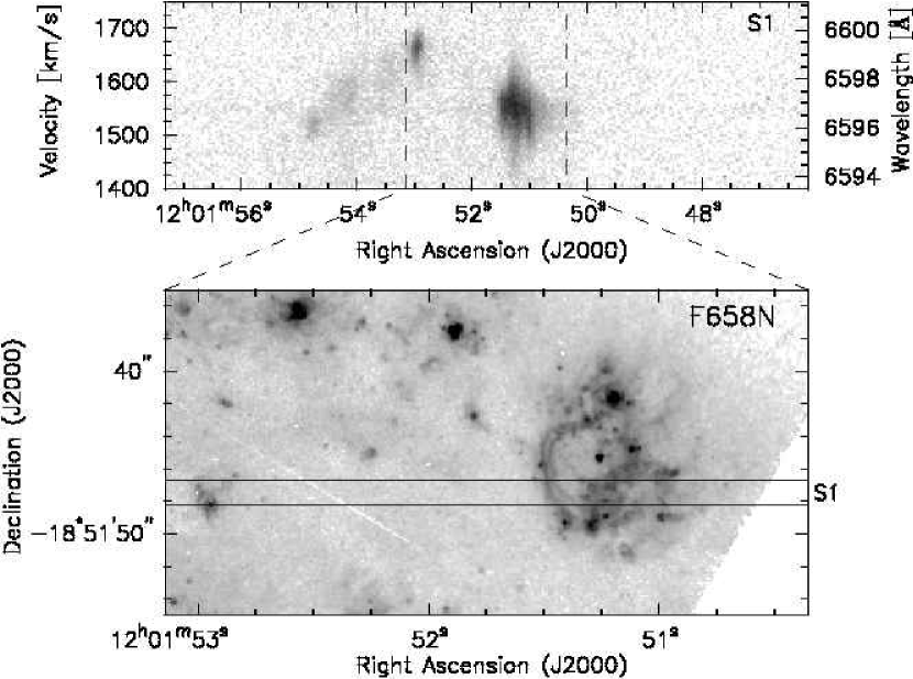
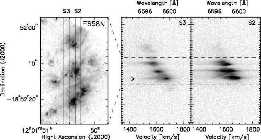
Figure 5: Echellograms of the H$\alpha$ line region at slit positions S1, S2, and S3 along with HST WFPC2 F658N images showing the location of the slit positions. Slit position S1 covers the supergiant shell in D03. Slit positions S2 and S3 sample the giant H II regions and their vicinities in D01 and D02. The arrow in the echellogram for the slit position S3 marks the high-velocity gas associated with a discrete soft X-ray source, suggesting a SNR candidate.

Active star formation regions often contain large interstellar shell structures; for example, region D01 contains a large shell structure extending from the two southern giant H II regions to the east with a diameter of $\sim$ 500 pc. This large shell is detected in our echelle observation at slit position S2 (see Figure 5). Its expansion velocity, $\sim 65$ km s^-1, is larger than most supershells of comparable sizes in dwarf galaxies (Martin, 1998). Six clusters exist in region D01, including a super-star cluster. Note that the ionized gas near the super-star cluster does not expand as fast as the supershell. Evidently, the super-star cluster is either in a denser ISM or has not injected sufficient energy to accelerate the ambient ISM.

It is interesting to note that the largest expansion velocities ($>$100 km s^-1) we detected in D01 are in regions outside the main body of the giant H II regions. See the echellograms at S2 and S3 in Figure 5. These high-velocity features are most likely associated with SNRs. Indeed, one high-velocity feature along S3, marked in Figure 5, is coincident with an unresolved soft X-ray source marked in Figure 1a as a SNR candidate.

Prolonged and spatially extended star formation activity may produce supergiant shells with sizes approaching 1,000 pc. Region D03 contains a supergiant shell which may be compared to LMC-2, the brightest supergiant shell in the Large Magellanic Cloud (LMC). LMC-2 is comparable to the D03 shell in linear size, but its X-ray luminosity is an order of magnitude lower (Points et al., 2001). In this case, the super-star cluster in the D03 supergiant shell must have played a significant role in the production of hot gas. Our echelle observations of this supergiant shell show larger velocity widths in the bright H II region on the shell rim than within the supergiant shell. Unfortunately, the spatial resolution of our echelle observations is much lower than that of the WFPC2 so the supergiant shell is not adequately resolved and only an upper limit of 50 km s^-1 can be placed on its expansion velocity.

6.2 Regions without Active Star Formation

Three of the diffuse X-ray emission regions we selected, D06, D08, and D11, contain no obvious star formation activity, as indicated by the H$\alpha$ image. The lack of active star formation in these regions is also indicated by CO maps (Liang et al., 2001) and mid-IR (12–18 $\mu$m) images (Mirabel & Laurent, 1999). No super-star clusters exist in D06 and D08, and no clusters are cataloged in D11 at all. The origin of the hot gas in these regions without active star formation is puzzling. It is clearly not powered by super-star clusters. It is unlikely that this hot gas is transported from neighboring star formation regions via breakouts, as these regions contain much more thermal energy than the regions with star formation or super-star clusters.

Not all massive stars are formed in clusters or super-clusters. In nearby galaxies where individual massive stars are resolved, it has been shown that giant H II regions may contain only loose OB associations without high concentrations, e.g., NGC 604 in M33 (Hunter et al., 1996), and that supergiant shells may be associated with wide-spread, low-surface-density star formation, e.g., Shapley Constellation III in LMC-4 (Shapley, 1956). Both NGC 604 and LMC-4 are diffuse X-ray sources with X-ray luminosities of 10³⁷–10³⁸ and $1.4\times 10^{37}$ ergs s^-1, respectively (Yang et al., 1996; Bomans et al., 1994). It is therefore possible that the hot gas in the Antennae regions without on-going active star formation was generated by field stars or low-mass clusters within the last $\sim$100 Myr

7 Summary

We have used $Chandra$ archival observations of NGC 4038/4039, the Antennae galaxies, to investigate the distribution and physical properties of the hot interstellar gas. Eleven distinct diffuse X-ray emission regions are selected according to their underlying interstellar structures and star formation activity; five contain giant H II regions, two are associated with circumnuclear starbursts, one is coincident with a supergiant shell, and three do not show active star formation. Their X-ray spectra are analyzed to determine the thermal energy content and cooling timescale.

To investigate the stellar energy input in these diffuse X-ray emission regions, we have identified the underlying young star clusters and used the evolutionary stellar population synthesis code Starburst99 to model their photometric magnitudes and colors in order to assess their initial masses and ages. The cluster masses and ages are then used to determine the stellar wind and supernova energies injected into the ISM in each region.

Comparisons between the thermal energy in the hot ISM and the expected stellar energy input show that in diffuse X-ray emission regions associated with active star formation, such as giant H II regions, circumnuclear starbursts, and supergiant shells, the underlying young star clusters play significant to dominant roles in heating the ISM. Super-star clusters with masses above $1\times 10^{5}$ M_⊙ contribute to the production of hot ISM, but the yield of hot gas is not linearly proportional to the cluster mass.

There are regions without active star formation where the hot gas cannot have been produced by young star clusters. We suggest that the hot gas in these regions without on-going active star formation may have been produced by field stars or low-mass clusters.

Appendix A Choosing a Spectral Model

The physical properties of an X-ray emitting plasma can be determined from the best model fit to the observed spectrum. To improve the spectral fits, models for diffuse X-ray sources frequently include multiple thermal plasma components and a power law component, the latter of which is argued to represent the emission from unresolved point sources. These complex models almost always lead to better fits with unrealistically low abundances, for example, NGC 253 (Strickland et al., 2002) and NGC 4631 (Wang et al., 2001). It is thus worthwhile to examine the effects and necessity of these spectral components.

We use the spectrum of region D06 to illustrate how models affect the results of spectral fitting. We have fit the spectrum with the following models: (1) single thermal plasma component, (2) two thermal plasma components, (3) single thermal plasma component plus a power law, and (4) two thermal plasma components plus a power law. For each of these models, we try spectral fits with floating and fixed plasma abundances, and with floating and fixed absorption column density. The MEKAL model (Kaastra & Mewe, 1993; Liedahl et al., 1995) is used for the thermal plasma emission, the absorption cross sections are from Balucińska-Church & McCammon (1992) and the solar abundances are adopted for the foreground absorption. The additional absorption due to the build-up on the ACIS-S is also modeled and taken into account in the spectral fits.

When we make spectral fits with floating absorption column density, the best-fits all converge to a column density much lower than the foreground Galactic absorption, which is unphysical. We have therefore adopted the Galactic H I column density of $3.9\times 10^{20}$ cm^-2 (Dickey & Lockman, 1990) as the absorption column density. The results discussed below are based on models using this fixed absorption column density.

For a single thermal plasma component model, the best spectral fit with floating abundances gives a plasma temperature of $kT$ = 0.55 keV but an unphysically low abundance of 0.14 Z_⊙. The best fit with an abundance fixed at the solar value gives a similar temperature, $kT$ = 0.55 keV, but the model underestimates emission at 0.5–0.6 keV and $\sim$1.5 keV. See the top two panels of Figure 6 for a comparison between spectral fits with abundances of 0.14 Z_⊙ and 1 Z_⊙. The 0.14 Z_⊙ model fits the observed spectrum better because the metal lines between 0.6 keV and 1 keV are suppressed so that the relative contribution from the bremsstrahlung emission can be raised to produce adequate emission below 0.6 keV.

For a model with two thermal plasma components each with independent floating abundances, the best fit converges to one component with $kT_{1}$ = 0.37 keV and abundances of 1.7 Z_⊙, and another component with higher temperature $kT_{2}$ = 0.71 keV and abundances of 0.7 Z_⊙. The middle-left panel of Figure 6 shows an example of a spectral fit with two thermal plasma components of different abundances. The spectra of the two plasma components are individually plotted to show their contributions to the total emission (middle-left panel of Figure 6). The lower temperature component prevails in the low energy band, while the higher temperature component dominates the $>$ 1 keV band.

For a model with two thermal plasma components of identical floating abundances, the best fit has temperatures $kT_{1}=$ 0.38 keV and $kT_{2}$ = 0.68 keV, but unphysically low abundances $Z$ = 0.19 $Z_{\odot}$. As in the above case, the higher temperature component dominates the $>$ 1 keV band (middle-right panel of Figure 6).

For a model with two thermal plasma components of solar abundances, the best fit converges to one component with $kT_{1}$ = 0.23 keV and a weaker component with $kT_{2}$ = 0.61 keV. The bottom-left panel of Figure 6 shows the spectra of these individual components. The main component accounts for the overall spectral shape, and the secondary component produces more emission below 0.6 keV.

Adding a power law component to the single thermal plasma component model, the best fit has a temperature, $kT$ $\sim$ 0.5 keV, similar to that of the model without a power law component, but the abundance is significantly higher, $Z$ = 1.2 $Z_{\odot}$. Fixing the abundance at the solar value, the best spectral fit also gives a temperature, $kT\sim$ 0.52 keV, similar to that of the model without a power law component. The contributions of the thermal plasma and power law components are illustrated in the bottom-right panel of Figure 6. It is evident that the power law component facilitates the fit by contributing to the soft X-ray emission.

Finally, using a model incorporating a power law component and two thermal components, the best fit shows a main thermal plasma component and a power law component similar to those for the above model with a single thermal plasma component and a power law component, and a secondary thermal component which makes a negligible contribution to the total emission.

It becomes clear from these results that the spectral ranges below and above 0.6 keV cannot be simultaneously fit well by a model with a single thermal plasma component at the solar abundance. The spectral fit below 0.6 keV can be improved by drastically lowering the abundance to suppress the metal lines above 0.6 keV, adding another thermal plasma component at a low temperature to boost the X-ray emission below 0.6 keV, or adding a power law component that rises toward the low energies.

Are these ad hoc fixes artificial? Abundances as low as 0.1 Z_⊙ are commonly found in dwarf galaxies such as the Small Magellanic Cloud, but not in gas-rich spirals such as the Antennae galaxies. Spectrophotometric observations of 18 H II regions in the Antennae show an [O III] $\lambda$5007 line comparable to or weaker than the H$\beta$ line (Rubin et al., 1970), which is consistent with low electron temperatures and high abundances. Moreover, the abundances of a dwarf galaxy in the tidal tail drawn from the outer parts of the Antennae are comparable to the LMC abundance (Mirabel et al., 1992), further supporting that the abundances of the inner parts of the Antennae should be solar or higher. Therefore, the X-ray spectral fits that require metallicities below 0.3 Z_⊙ can be ruled out.

The addition of a power law component is also not justified because the diffuse X-ray emission from the Antennae galaxies is associated with star formation regions and is not expected to include a significant contribution from faint, unresolved point sources of X-ray binaries. For example, $ROSAT$ observations of the LMC (at 50 kpc) show that X-ray binaries brighter than 10³⁴ ergs s^-1 are rare in star forming regions and no power law component is needed in the analysis of the diffuse X-ray emission (Chu, 1998; Chu & Snowden, 1998; Points et al., 2001).

As it is not even clear whether the ACIS-S spectra in the soft energy range are accurately calibrated (Strickland et al., 2002), it is premature to include multiple components and adhere to the absolute least-$\chi^{2}$ for the best model fit. Therefore, we have chosen to analyze the spectra with only one single thermal plasma component at a fixed abundance, $Z=Z_{\odot}$.

It is possible that the abundance is higher or lower than the solar value. As the X-ray emissivity scales directly with the abundance $Z$, the normalization factor of the spectral fit, or the volume emission measure, will scale with $Z^{-1}$. Consequently, the rms density, mass, and thermal energy of the X-ray-emitting plasma all scale with $Z^{-1/2}$. Thus the uncertainties in the mass and thermal energy are not as large as the uncertainty in the abundance itself.

Appendix B Comparisons among Different Models

Following the referee’s suggestion, we compare the goodness-of-fit among different models and show how these different models affect the thermal energy of the hot gas. First we carry out single-component MEKAL model fits with fixed solar abundances and with floating (free-varying) abundances for all 11 diffuse emission regions. The results are presented in Table 6. By allowing the abundances to vary freely and converge at very low abundances, $\sim 0.1~{}Z_{\odot}$, the goodness-of-fit can be significantly improved. Compared to the best-fit models with fixed solar abundance, the best-fit models with free-varying abundances have similar temperatures but the thermal energies are 2–4 times higher. The thermal energies are raised because higher densities are needed to compensate for the low abundances in order to produce the observed emission, and higher densities lead to larger thermal energies. The density and thermal energy roughly scale with $Z^{-1/2}$, as explained at the end of Appendix A,

As we discussed in Appendix A, abundances as low as 0.1 $Z_{\odot}$ can be excluded for the Antennae galaxies because even the outer parts of the Antennae have higher abundances (Mirabel et al., 1992). Thus, we next consider one-component and 2-component MEKAL models with solar abundances for all 11 diffuse X-ray sources. The results are presented in Table 7. The goodness-of-fit is improved in the 2-component model fits. The two temperatures in the 2-component model fits bracket the temperatures of the corresponding 1-component model fits. In some of the cases, the second component has unrealistically high temperatures, which may be caused by low S/N in the data or simply deficiencies of the MEKAL model. When the two temperatures of the 2-component model are reasonable, the resulting thermal energy is higher, but not more than a factor of 2 higher, than that of the corresponding 1-component model. This difference does not affect the conclusions of our comparison between stellar energy input and the thermal energy in §5.4.

Finally, we compare spectral fits made with the APEC (Astrophysical Plasma Emission Code) model (Smith et al., 2001) and with the MEKAL model. Two temperature components are used with solar abundances. The results are presented in Table 8. The APEC spectral fits are generally consistent with the MEKAL spectral fits, and the resultant thermal energies are similar, although the APEC models fit the spectra better (smaller reduced $\chi^{2}$), and give more reasonable temperatures even when MEKAL models produce unrealistically high temperatures. Note that the APEC models still produce very high temperatures for D05, D09, and D11, which might be due to the low S/N in the spectra of D05 and D09 and uncertain origins of the hot gas in D11.

Figure 3: Spectra and best-fit models of the 11 regions with diffuse X-ray emission. The regions are listed in Table 1 and described in §3. The adopted spectral model consists of a single-temperature MEKAL model with a fixed solar abundance. The spectra and best fits are shown in the upper panels, and the residuals of the fits in units of $\sigma$ for each energy bin are shown in the lower panels.

Figure 4: (a) Reddening-free color-color diagram for $Q_{1}$ versus $Q_{3}$. The 50 young star clusters from Table 1 of Whitmore et al. (1999) are plotted as solid circles. The evolutionary track produced by Starburst99 for a cluster with solar abundance is plotted with ages marked every Myr as solid squares. (b) Reddening-free color-magnitude diagrams for $W$ versus $Q_{1}$ and $W$ versus $Q_{3}$. The evolutionary track for a cluster of initial masses of $5\times 10^{5}$ M_⊙ in the $W$–$Q_{1}$ diagram is plotted in solid curve, and that for a $5\times 10^{4}$ M_⊙ cluster is plotted in the $W$–$Q_{3}$ diagram in dashed curve. (Different masses are used in these two evolutionary tracks to offset the curves vertically for clarity.) The cluster ages are marked along the evolutionary tracks in 2 Myr intervals. (c) Reddening-free color-magnitude diagram for $W$ versus $Q_{1}$. The 50 young star clusters from Table 1 of Whitmore et al. (1999) are plotted as solid circles. Evolutionary tracks for clusters of initial masses of $5\times 10^{4}$, $1\times 10^{5}$, and $5\times 10^{5}$ M_⊙ are plotted . (d) same as (c) for $W$ versus $Q_{3}$.

Figure 6: Spectral fits for region D06 using different models. As in Figure 3, the top panel shows the spectra and spectral fits, and the bottom panel shows the residuals in units of $\sigma$ for each energy bin. The model and the best-fit parameters are labeled in each panel. For spectral fits with more than one component, the individual components and their sum are all shown.

Table 1: Regions of Diffuse X-ray Sources in the Antennae Galaxies

Region	R.A.	Dec	Size	P.A.	$V$	Counts	Apparent
	(J2000)			(∘)	(pc3)		Association
D01	12 01 50.51	$-$18 52 17.9	14$\farcs$8$\times$ 9$\farcs$8	160	6.0$\times$108	1150	Giant H II region
D02	12 01 50.55	$-$18 52 05.1	9$\farcs$8$\times$ 5$\farcs$9	160	1.4$\times$108	375	Giant H II region
D03	12 01 51.29	$-$18 51 46.6	15$\farcs$7$\times$11$\farcs$8	10	9.2$\times$108	470	Supergiant shell
D04	12 01 52.96	$-$18 52 03.3	7$\farcs$9$\times$ 5$\farcs$9	125	1.1$\times$108	355	Circumnuclear H II
D05	12 01 52.96	$-$18 52 09.5	6$\farcs$9$\times$ 6$\farcs$9	$\cdots$	1.3$\times$108	410	Circumnuclear H II
D06	12 01 53.43	$-$18 51 53.0	25$\farcs$3$\times$16$\farcs$0	140	2.7$\times$109	1950	$\cdots$
D07	12 01 54.47	$-$18 52 10.0	18$\farcs$1$\times$ 9$\farcs$8	120	7.0$\times$108	790	Giant H II region
D08	12 01 56.13	$-$18 52 27.0	23$\farcs$6$\times$11$\farcs$8	130	1.4$\times$109	1320	$\cdots$
D09	12 01 55.33	$-$18 52 48.9	8$\farcs$9$\times$ 5$\farcs$9	130	1.2$\times$108	275	Giant H II region
D10	12 01 54.40	$-$18 53 04.1	11$\farcs$8$\times$ 7$\farcs$9	130	2.9$\times$108	800	Giant H II region
D11	12 01 54.08	$-$18 53 09.0	21$\farcs$6$\times$ 5$\farcs$9	130	3.2$\times$108	1620	$\cdots$

Table 2: Results of X-ray Spectral Fits

Region	$T$	$kT$	$A$	rms $N_{\rm e}$	$f^{\rm obs}_{\rm X}$ (0.5–2.0 keV)	$L_{\rm X}$ (0.5–2.0 keV)
	(106 K)	(keV)	(cm-5)	(cm-3)	(ergs cm-2 s-1)	(1038 ergs s-1)
D01	4.3$\pm$0.5	0.37$\pm$0.04	9.9$\times$10-6	0.05	2.0$\times$10-14	13.0
D02	4.5$\pm$1.0	0.39$\pm$0.09	3.1$\times$10-6	0.06	6.5$\times$10-15	4.1
D03	6.7$\pm$1.0	0.58$\pm$0.09	3.5$\times$10-6	0.02	8.3$\times$10-15	5.1
D04	8.6$\pm$0.9	0.74$\pm$0.08	2.7$\times$10-6	0.06	6.3$\times$10-15	3.8
D05	7.2$\pm$0.9	0.62$\pm$0.08	2.9$\times$10-6	0.06	6.9$\times$10-15	4.2
D06	6.3$\pm$0.8	0.54$\pm$0.07	1.4$\times$10-5	0.03	3.3$\times$10-14	20.0
D07	7.2$\pm$0.5	0.62$\pm$0.04	5.2$\times$10-6	0.03	1.3$\times$10-14	7.7
D08	6.7$\pm$0.6	0.58$\pm$0.05	9.2$\times$10-6	0.03	2.2$\times$10-14	13.0
D09	7.3$\pm$1.2	0.63$\pm$0.10	1.7$\times$10-6	0.04	4.1$\times$10-15	2.5
D10	7.8$\pm$0.6	0.67$\pm$0.05	5.7$\times$10-6	0.05	1.3$\times$10-14	8.2
D11	7.7$\pm$0.4	0.66$\pm$0.03	1.2$\times$10-5	0.08	2.8$\times$10-14	17.0

Table 3: Energies and Cooling Timescales of Diffuse X-ray Emission Regions

Region	Young Star	$E_{\rm th}$	$E_{\star}$ Input	$E_{\star}$ Input	$t_{\rm cool}$
	Clusters	(ergs)	(ergs)	(ergs)	(Myr)
D01	2,22,29,31,40,46	1.5$\times$1054	1.4$\times$1054	1.4$\times$1054	65
D02	12,47,50	4.3$\times$1053	1.0$\times$1054	8.1$\times$1053	55
D03	1,43,44	1.7$\times$1054	5.6$\times$1054	6.7$\times$1054	240
D04	34,38	6.6$\times$1053	4.0$\times$1054	3.4$\times$1054	105
D05	3,4	6.2$\times$1053	3.8$\times$1054	3.3$\times$1054	90
D06	42	5.5$\times$1054	1.0$\times$1053	1.1$\times$1053	150
D07	7,13,18,41	1.9$\times$1054	1.8$\times$1054	1.3$\times$1054	175
D08	35,48	3.4$\times$1054	9.4$\times$1053	1.1$\times$1054	140
D09	17,19	4.5$\times$1053	9.5$\times$1053	7.8$\times$1053	130
D10	9,11,14,20,26,30,33,39	1.4$\times$1054	8.6$\times$1054	5.1$\times$1054	115
D11	$\cdots$	2.2$\times$1054	$\cdots$	$\cdots$	70

Table 4: Stellar Wind and Supernova Energies of Young Star Clusters

Cluster	$M_{\rm cluster}$	$t_{\rm cluster}$	$M_{\rm min}$	$N_{\rm SN}$	$E_{\rm SN}$	$E_{\rm wind}$	$E_{\rm SN}$	$E_{\rm wind}$	Region
	(M⊙)	(Myr)	(M⊙)		($\times$1053 ergs)
1	5$\times$105	14.0	13.9	4300	43	4.8	42.9	15.1	D03
2	1$\times$105	7.0	18.3	580	5.8	0.96	3.4	3.0	D01
3	4$\times$105	6.0	19.4	2100	21	3.8	10.0	11.9	D05
4	2$\times$105	6.0	19.4	110	11	1.9	5.0	6.0	D05
5	1.5$\times$105	4.0	22.9	610	6.1	1.4	1.0	2.6	$\cdots$
6	1.2$\times$105	14.0	13.9	1000	10	1.1	10.3	3.6	D02
7	1.2$\times$105	5.5	20.1	600	6.0	1.1	2.5	3.4	D07
8	1.5$\times$105	5.5	20.1	750	7.5	1.4	3.1	4.2	$\cdots$
9	3$\times$105	3.5	24.1	1100	11	2.9	0	4.1	D10
10	1.5$\times$105	13.0	14.3	1200	12	1.4	11.9	4.5	$\cdots$
11	5$\times$105 ?	6 ?	19.4	2600	26	4.8	12.6	14.9	D10
12	1$\times$105	6.0	19.4	530	5.3	0.96	2.5	3.0	D02
13	7$\times$104	5.0	20.9	330	3.3	0.67	1.1	1.7	D07
14	3$\times$105	3.0	25.7	1000	10	2.9	0	3.0	D10
15	5$\times$104	7.5	17.8	300	3.0	0.48	1.9	1.5	$\cdots$
16	2$\times$105	14.0	13.9	1700	17	1.9	17.1	6.0	$\cdots$
17	1$\times$105	5.5	20.1	500	5.0	0.96	2.1	2.8	D09
18	1.2$\times$105	4.0	22.9	490	4.9	1.1	0.8	2.1	D07
19	6$\times$104	5.5	20.1	300	3.0	0.57	1.2	1.7	D09
20	3$\times$105	3.0	25.7	1000	10	2.9	0	3.0	D10
21	5$\times$104	5.5	20.1	250	2.5	0.48	1.0	1.4	$\cdots$
22	1.5$\times$104	7.5	17.8	90	0.90	0.14	0.6	0.5	D01
23	8$\times$104	5.5	20.1	400	4.0	0.77	1.6	2.2	$\cdots$
24	7$\times$104	14.0	13.9	610	6.1	0.67	6.0	2.1	$\cdots$
25	1$\times$105	3.5	24.1	380	3.8	0.99	0	1.4	$\cdots$
26	3.5$\times$104	7.5	17.8	210	2.1	0.34	1.4	1.1	D10
27	7$\times$104	14.0	13.8	610	6.1	0.67	6.0	2.1	$\cdots$
28	8$\times$104	5.5	20.1	400	4.0	0.77	1.6	2.2	$\cdots$
29	2$\times$104	8.0	17.3	120	1.2	0.19	0.9	0.6	D01
30	7$\times$104	5.5	20.1	350	3.5	0.67	1.4	2.0	D10
31	1$\times$104	7.5	17.8	60	0.60	0.096	0.4	0.3	D01
32	5$\times$104	4.0	22.9	200	2.0	0.48	0.3	0.9	$\cdots$
33	7$\times$104	6.5	18.8	390	3.9	0.67	2.1	2.1	D10
34	3$\times$105	6.0	18.5	1700	17	2.9	7.5	9.0	D04
35	2$\times$104	7.5	17.8	120	1.2	0.19	0.8	0.6	D08
36	3$\times$105	14.0	13.9	2600	26	2.9	25.7	9.1	$\cdots$
37	1.5$\times$104	7.5	17.8	90	0.90	0.14	0.6	0.5	$\cdots$
38	3$\times$105	6.5	18.8	1700	17	2.9	8.9	9.0	D04
39	7$\times$104	5.5	20.1	350	3.5	0.67	1.4	2.0	D10
40	5$\times$104	6.0	19.4	260	2.6	0.48	1.3	1.5	D01
41	1.2$\times$104	7.5	17.8	72	0.72	0.11	0.5	0.4	D07
42	1.5$\times$104	7.5	17.8	90	0.90	0.14	0.6	0.5	D06
43	5$\times$104	14.0	13.9	430	4.3	0.48	4.3	1.5	D03
44	5$\times$104	7.5	17.8	300	3.0	0.48	1.9	1.5	D03
45	7$\times$104	6.0	19.4	370	3.7	0.67	1.8	2.1	$\cdots$
46	2$\times$104	6.5	18.8	110	1.1	0.19	0.6	0.6	D01
47	4$\times$104	6.0	19.4	210	2.1	0.38	1.0	1.2	$\cdots$
48	8$\times$104	15.0	13.5	720	7.2	0.77	7.3	2.4	D08
49	8$\times$104	6.0	19.4	420	4.2	0.77	2.0	2.4	$\cdots$
50	1$\times$104	7.5	17.8	60	0.60	0.096	0.4	0.3	D02

Table 5: Upper Limits for Stellar Wind Energy

Type	Mass	$v_{\infty}$	$E_{\rm wind}$
	(M⊙)	(km s-1)	(ergs)
O3	120	3,150	5.9$\times$1051
O5	60	1,885	1.1$\times$1051
O8	23	1,530	2.7$\times$1050
B0	17.5	1,535	2.1$\times$1050
B3	7.6	590	1.3$\times$1049

Table 6: One-Component MEKAL Models with Solar and Free-Varying Abundances

Region	Solar Abundance			Free-Varying Abundances
	$kT$	$\chi^{2}$/DoF	$E_{\rm th}$	$kT$	$Z$	$\chi^{2}$/DoF	$E_{\rm th}$
	(keV)		(ergs)	(keV)	($Z_{\odot}$)		(ergs)
D01	0.37	126.7/28 = 4.5	1.5$\times 10^{54}$	0.43	0.06	58.6/27 = 2.2	5.2$\times 10^{54}$
D02	0.37	20.5/ 8 = 2.6	4.3$\times 10^{53}$	0.40	0.04	7.0/ 7 = 1.0	1.6$\times 10^{54}$
D03	0.58	36.2/13 = 2.8	1.7$\times 10^{54}$	0.53	0.07	9.1/12 = 0.8	4.6$\times 10^{54}$
D04	0.76	47.6/10 = 4.8	7.2$\times 10^{53}$	0.78	0.13	23.8/ 9 = 2.6	1.6$\times 10^{54}$
D05	0.61	46.2/10 = 4.6	6.2$\times 10^{53}$	0.64	0.05	11.3/ 9 = 1.3	2.0$\times 10^{54}$
D06	0.54	189.4/42 = 4.5	5.6$\times 10^{54}$	0.53	0.10	88.7/41 = 2.2	1.4$\times 10^{55}$
D07	0.62	121.5/21 = 5.9	2.0$\times 10^{54}$	0.61	0.08	59.0/20 = 2.9	5.5$\times 10^{54}$
D08	0.58	144.4/33 = 4.4	3.6$\times 10^{54}$	0.58	0.10	61.4/32 = 1.9	9.4$\times 10^{54}$
D09	0.62	47.9/ 6 = 8.0	4.8$\times 10^{53}$	0.71	0.02	8.8/ 5 = 1.8	1.9$\times 10^{54}$
D10	0.67	82.9/22 = 3.8	1.5$\times 10^{54}$	0.68	0.12	28.6/21 = 1.4	3.6$\times 10^{54}$
D11	0.66	93.5/38 = 2.5	2.2$\times 10^{54}$	0.67	0.21	51.7/37 = 1.4	4.4$\times 10^{54}$

Table 7: One- versus Two-Component MEKAL Models with Solar Abundance

Region	One-Component			Two-Component
	$kT$	$\chi^{2}$/DoF	$E_{\rm th}$	$kT_{1}$	$kT_{2}$	$\chi^{2}$/DoF	$E_{\rm th}$
	(keV)		(ergs)	(keV)	(keV)		(ergs)
D01	0.37	126.7/28 = 4.5	1.5$\times 10^{54}$	0.22	0.63	52.7/26 = 2.0	2.8$\times 10^{54}$
D02	0.37	20.5/ 8 = 2.6	4.3$\times 10^{53}$	0.18	0.56	7.0/ 6 = 1.2	7.1$\times 10^{53}$
D03	0.58	36.2/13 = 2.8	1.7$\times 10^{54}$	0.19	0.64	9.8/11 = 0.9	2.2$\times 10^{54}$
D04	0.76	47.6/10 = 4.8	7.2$\times 10^{53}$	0.70	6.6	8.3/ 8 = 1.0	8.1$\times 10^{54}$
D05	0.61	46.2/10 = 4.6	6.2$\times 10^{53}$	0.57	3.4	8.6/ 8 = 1.1	4.9$\times 10^{54}$
D06	0.54	189.4/42 = 4.5	5.6$\times 10^{54}$	0.23	0.61	119.1/40 = 3.0	7.5$\times 10^{54}$
D07	0.62	121.5/21 = 5.9	2.0$\times 10^{54}$	0.23	0.70	79.8/19 = 4.2	2.7$\times 10^{54}$
D08	0.58	144.4/33 = 4.4	3.6$\times 10^{54}$	0.32	0.85	80.6/32 = 2.5	5.7$\times 10^{54}$
D09	0.62	47.9/ 6 = 8.0	4.8$\times 10^{53}$	0.56	6.6	9.8/ 4 = 2.5	8.8$\times 10^{54}$
D10	0.67	82.9/22 = 3.8	1.5$\times 10^{54}$	0.61	1.5	40.7/20 = 2.0	3.8$\times 10^{54}$
D11	0.66	93.5/38 = 2.5	2.2$\times 10^{54}$	0.63	3.5	48.5/36 = 1.3	1.1$\times 10^{55}$

Table 8: Two-Component MEKAL versus APEC with Solar Abundance

Region	Two-Component MEKAL				Two-Component APEC
	$kT_{1}$	$kT_{2}$	$\chi^{2}$/DoF	$E_{\rm th}$	$kT_{1}$	$kT_{2}$	$\chi^{2}$/DoF	$E_{\rm th}$
	(keV)	(keV)		(ergs)	(keV)	(keV)		(ergs)
D01	0.22	0.63	52.7/26 = 2.0	2.8$\times 10^{54}$	0.24	0.70	51.3/26 = 2.0	2.8$\times 10^{54}$
D02	0.18	0.56	7.0/ 6 = 1.2	7.1$\times 10^{53}$	0.18	0.57	3.7/ 6 = 0.7	7.5$\times 10^{53}$
D03	0.19	0.64	9.8/11 = 0.9	2.2$\times 10^{54}$	0.18	0.64	6.1/11 = 0.6	2.3$\times 10^{54}$
D04	0.70	6.6	8.3/ 8 = 1.0	8.1$\times 10^{54}$	0.41	0.97	34.6/ 8 = 4.3	1.1$\times 10^{54}$
D05	0.57	3.4	8.6/ 8 = 1.1	4.9$\times 10^{54}$	0.59	2.6	7.5/ 8 = 0.9	3.8$\times 10^{54}$
D06	0.23	0.61	119.1/40 = 3.0	7.5$\times 10^{54}$	0.21	0.61	85.7/40 = 2.1	7.7$\times 10^{54}$
D07	0.23	0.70	79.8/19 = 4.2	2.7$\times 10^{54}$	0.22	0.69	62.6/19 = 3.3	2.7$\times 10^{54}$
D08	0.32	0.85	80.6/32 = 2.5	5.7$\times 10^{54}$	0.33	0.80	66.3/32 = 2.1	5.8$\times 10^{54}$
D09	0.56	6.6	9.8/ 4 = 2.5	8.8$\times 10^{54}$	0.59	4.9	8.9/ 4 = 2.2	6.7$\times 10^{54}$
D10	0.61	1.5	40.7/20 = 2.0	3.8$\times 10^{54}$	0.25	0.76	52.9/20 = 2.6	2.0$\times 10^{54}$
D11	0.63	3.5	48.5/36 = 1.3	1.1$\times 10^{55}$	0.65	2.1	36.6/36 = 1.0	6.9$\times 10^{54}$

References

- Arnaud (1996) Arnaud, K. A. 1996, ASP Conf. Ser. 101: Astronomical Data Analysis Software and Systems V, 5, 17
- Balucińska-Church & McCammon (1992) Balucinska-Church, M., & McCammon, D. 1992, ApJ, 400, 699
- Binney & Merrifield (1998) Binney, J. & Merrifield, M. 1998, Galactic Astronomy (Princeton, NJ: Princeton University Press)
- Bomans et al. (1994) Bomans, D. J., Dennerl, K., & Kürster, M. 1994, A&A, 283, L21
- Bruzual & Charlot (2003) Bruzual, G., & Charlot, S. 2003, MNRAS, 344, 1000
- Chen, Chu, & Johnson (2004) Chen, C.-H. R., Chu, Y.-H., & Johnson, K. E. 2004, in preparation
- Chu (1998) Chu, Y.-H. 1998, The Magellanic Clouds and Other Dwarf Galaxies, Proceedings of the Bonn/Bochum-Graduiertenkolleg Workshop, eds. T. Richtler & J. M. Braun, p. 11
- Chu & Snowden (1998) Chu, Y.-H. & Snowden, S. L. 1998, Astronomische Nachrichten, vol. 319, no. 1, p. 101
- Cooper et al. (2004) Cooper, R. L., Guerrero, M. A., Chu, Y.-H., Chen, C.-H. R., & Dunne, B. C. 2004, ApJ, submitted
- Dalgarno & McCray (1972) Dalgarno, A., & McCray, R. A. 1972, ARA&A, 10, 375
- Dickey & Lockman (1990) Dickey, J. M., & Lockman, F. J. 1990, ARA&A, 28, 215
- Fabbiano et al. (1982) Fabbiano, G., Feigelson, E., & Zamorani, G. 1982, ApJ, 256, 397
- Fabbiano et al. (2003) Fabbiano, G., Krauss, M., Zezas, A., Rots, A., & Neff, S. 2003, ApJ, 598, 272
- Fabbiano et al. (1997) Fabbiano, G., Schweizer, F., & Mackie, G. 1997, ApJ, 478, 542
- Fabbiano & Trinchieri (1983) Fabbiano, G., & Trinchieri, G. 1983, ApJ, 266, L5
- Fabbiano et al. (2001) Fabbiano, G., Zezas, A., & Murray, S. S. 2001, ApJ, 554, 1035
- Hunter et al. (1996) Hunter, D. A., Baum, W. A., O’Neil, E. J., Jr., & Lynds, R. 1996, ApJ, 456, 174
- Kaastra & Mewe (1993) Kaastra, J. S., & Mewe, R. 1993, Legacy, 3, 16, HEASARC, NASA
- Kim et al. (1998) Kim, S., Chu, Y.-H., Staveley-Smith, L., & Smith, R. C. 1998, ApJ, 503, 729
- Kuntz et al. (2003) Kuntz, K. D., Snowden, S. L., Pence, W. D., & Mukai, K. 2003, ApJ, 588, 264
- Leitherer et al. (1999) Leitherer, C. et al. 1999, ApJS, 123, 3
- Leitherer et al. (1992) Leitherer, C., Robert, C., & Drissen, L. 1992, ApJ, 401, 596
- Liang et al. (2001) Liang, M. C., Geballe, T. R., Lo, K. Y., & Kim, D.-C. 2001, ApJ, 549, L59
- Liedahl et al. (1995) Liedahl, D. A., Osterheld, A. L., & Goldstein, W. H. 1995, ApJ, 438, L115
- Madore (1982) Madore, B. F. 1982, ApJ, 253, 575
- Martin (1998) Martin, C. L. 1998, ApJ, 506, 222
- Mirabel et al. (1992) Mirabel, I. F., Dottori, H., & Lutz, D. 1992, A&A, 256, L19
- Mirabel & Laurent (1999) Mirabel, I. F. & Laurent, O. 1999, Ap&SS, 269, 349
- Points et al. (2001) Points, S. D., Chu, Y.-H., Snowden, S. L., & Smith, R. C. 2001, ApJS, 136, 99
- Prinja et al. (1990) Prinja, R. K., Barlow, M. J., & Howarth, I. D. 1990, ApJ, 361, 607
- Read et al. (1995) Read, A. M., Ponman, T. J., & Wolstencroft, R. D. 1995, MNRAS, 277, 397
- Rubin et al. (1970) Rubin, V. C., Ford, W. K. J., & D’Odorico, S. 1970, ApJ, 160, 801
- Salpeter (1955) Salpeter, E. E. 1955, ApJ, 121, 161
- Sansom et al. (1996) Sansom, A. E., Dotani, T., Okada, K., Yamashita, A., & Fabbiano, G. 1996, MNRAS, 281, 48
- Shapley (1956) Shapley, H. 1956, Am. Sci., 44, 73
- Smith et al. (2001) Smith, R. K., Brickhouse, N. S., Liedahl, D. A., & Raymond, J. C. 2001, ApJ, 556, L91
- Strickland et al. (2002) Strickland, D. K., Heckman, T. M., Weaver, K. A., Hoopes, C. G., & Dahlem, M. 2002, ApJ, 568, 689
- Wang et al. (2001) Wang, Q. D., Immler, S., Walterbos, R., Lauroesch, J. T., & Breitschwerdt, D. 2001, ApJ, 555, L99
- Whitmore & Zhang (2002) Whitmore, B. C. & Zhang, Q. 2002, AJ, 124, 1418
- Whitmore et al. (1999) Whitmore, B. C., Zhang, Q., Leitherer, C., Fall, S. M., Schweizer, F., & Miller, B. W. 1999, AJ, 118, 1551
- Williams & Chu (1995) Williams, R. M., & Chu, Y.-H. 1995, ApJ, 439, 132
- Yang et al. (1996) Yang, H., Chu, Y.-H., Skillman, E. D., & Terlevich, R. 1996, AJ, 112, 146
- Zhang et al. (2001) Zhang, Q., Fall, S. M., & Whitmore, B. C. 2001, ApJ, 561, 727
- Zezas et al. (2002a) Zezas, A., Fabbiano, G., Rots, A. H., Murray, S. S. 2002a, ApJS, 142, 239
- Zezas et al. (2002b) Zezas, A., Fabbiano, G., Rots, A. H., Murray, S. S. 2002b, ApJ, 577, 710