Strong Gravitational Lensing and Dark Energy Complementarity

Abstract

In the search for the nature of dark energy most cosmological probes measure simple functions of the expansion rate. While powerful, these all involve roughly the same dependence on the dark energy equation of state parameters, with anticorrelation between its present value $w_{0}$ and time variation $w_{a}$. Quantities that have instead positive correlation and so a sensitivity direction largely orthogonal to, e.g., distance probes offer the hope of achieving tight constraints through complementarity. Such quantities are found in strong gravitational lensing observations of image separations and time delays. While degeneracy between cosmological parameters prevents full complementarity, strong lensing measurements to 1% accuracy can improve equation of state characterization by 15-50%. Next generation surveys should provide data on roughly $10^{5}$ lens systems, though systematic errors will remain challenging.

I Introduction

Dark energy poses a fundamental challenge to our understanding of the universe. The acceleration of the cosmic expansion discovered through the Type Ia supernovae distance-redshift relation can be interpreted in terms of a new component of the energy density possessing a substantially negative pressure. Further observations from the cosmic microwave background radiation indicate the spatial geometry of the universe is flat; in combination with the supernova measurements this implies that the unknown “dark energy” comprises roughly 70% of the total density, in concordance with large scale structure data indicating that matter contributes approximately 30% of the critical density.

Such a weight of dark energy leads to its dominance of the expansion, causing acceleration, restricting the growth of large scale structure, and holding the key to the fate of the universe. But apart from its rough magnitude, its nature is almost unknown – whether it arises from the physics of the high energy vacuum, a scalar field, extra dimensional or “beyond Einstein” gravitational effects, etc. One way to gain clues to the underlying physical mechanism is to characterize the behavior of dark energy in terms of its equation of state ratio as a function of redshift (essentially a time parameter), $w(z)$. This is conventionally interpreted in terms of the ratio of the dark energy pressure to energy density, but can also be used as an effective parameterization to treat generalizations of the cosmology framework of the Friedmann equations of expansion linjen or simply in terms of the expansion rate and acceleration itself lingrav .

To obtain the clearest focus on the class of physics responsible for the accelerating universe, we seek the tightest constraints on the equation of state. This must come not merely from high statistical precision of a probe, but from robust control of systematic uncertainties. The greatest accuracy and confidence in the measurements will come from independent crosschecks and complementarity between methods of probing the cosmology. Many studies have considered such complementarity between probes (e.g. fhlt ; linap ; seo ; linbo ; wl ; cluster ), with a promising future for next generation surveys carrying out such measurements. However, all the methods of supernova distances, cosmic microwave background power spectrum, weak gravitational lensing, cluster counts, and baryon oscillations possess a similar fundamental dependence on the equation of state through the Hubble parameter, or expansion rate.

This paper investigates whether a truly complementary probe exists that has nearly orthogonal dependence to the previous ones in the plane of the equation of state parameters of value today, $w_{0}$, vs. time variation, $w_{a}$. Such a probe, if practical, would offer a valuable contribution to uncovering fundamental physics and deserve further consideration among next generation experiments. Section II considers the characteristics such a method would possess and identifies two promising candidates related to strong gravitational lensing. In §III we analyze the sensitivity of these probes to the cosmological parameters and the constraints and complementarity they offer. In the conclusion we summarize the prospects for strong lensing as a cosmological probe and discuss some issues regarding surveys and systematic uncertainties.

II Complementarity in the Equation of State Plane

Astronomical observations involving distances and volumes all follow from the metric in a simple, kinematic way weinberg . For convenience, the dependence can be written in terms of the conformal distance interval

$$d\eta=dt/a(t)=-dz/H(z),$$ (1)

where $a(t)=(1+z)^{-1}$ is the scale factor as a function of proper time, equivalently parametrized in terms of redshift $z$, and $H=\dot{a}/a$ is the Hubble parameter. So in observing some source at redshift $z$ the cosmological information is carried by the quantity $H$.

Varieties of distance observations – angular diameter, luminosity, proper motion – all contain the same information. One exception is the parallax distance (cf. fpoc , §3.2) which involves not only $H$ but the spatial curvature $k$ as well; however this is not practical for cosmology and CMB measurements strongly indicate a flat universe. Another subtlety involves exotic models that break the thermodynamic, or reciprocity, relation between the various distances thermo ; tolman ; bassett by violation of Liouville’s theorem, but this arises from photon properties and not cosmology.

Volume elements, and hence numbers of sources, are built up out of distances and so similarly involve the Hubble parameter. From the Friedmann equation the relation between the expansion rate and the dark energy equation of state is

$$H^{2}/H_{0}^{2}=\Omega_{m}(1+z)^{3}+\Omega_{DE}e^{3\int d\ln(1+z)\,[1+w(z)]},$$ (2)

where $H_{0}$ is the present value of the Hubble parameter (the Hubble constant), and for a flat universe $\Omega_{DE}=1-\Omega_{m}$. As discussed in linjen this can be written more generally as defining an effective equation of state

$$w(z)=-1+\frac{1}{3}\frac{d\ln\delta H^{2}/H_{0}^{2}}{d\ln(1+z)},$$ (3)

where $\delta H^{2}$ encodes our ignorance of the right hand side of eq. 2 after the first, matter density term.

Making $w(z)$ more positive (holding $H_{0}$ and $\Omega_{m}$ fixed) increases the expansion rate in the past, and so decreases the acceleration (since the rate today is fixed). Distances will be less, sources appear brighter, etc. If we try to characterize the nature of the dark energy in the simplest, nontrivial way, through the value of its equation of state today and its increasing or decreasing positivity into the past, we see that cosmological measurements, depending only on $H$, don’t really care in a gross sense how $w(z)$ was more positive – either increasing the present value $w_{0}$ or increasing the time variation $w_{a}\sim dw/d\ln(1+z)$ does the trick. Thus, for all such probes the quantities $w_{0}$, $w_{a}$ will be anticorrelated; an increase in one can be (at least partially) offset by a decrease in the other. If we plot constraints from astronomical data in the $w_{0}-w_{a}$ plane (marginalizing over any other parameters), the probability contours will show a degeneracy direction tilted counterclockwise from the vertical. This is well known and illustrated for a number of different probes in hutcoo ; note also that a “bare” $H$ of course has the same dependence linbo .

However, this has the fundamental implication that complementarity between methods can only be partial in this physically key parameter plane; different data sets cannot be orthogonal. This restricts the ability to constrain the equation of state and understand the nature of dark energy. What would be valuable is construction of a cosmological probe whose sensitivity lies clockwise of vertical, into the unexplored half-plane of positive correlation between $w_{0}$ and $w_{a}$. Note that this argument does not depend on the specifics of how $w_{0}$, $w_{a}$ are defined, but for concreteness we adopt the parametrization

$$w(z)=w_{0}+w_{a}(1-a)=w_{0}+w_{a}z/(1+z),$$ (4)

successful in fitting smoothly varying dark energy models linprl ; lin10217 . A characteristic time variation of the equation of state is given by $w^{\prime}\equiv dw/d\ln(1+z)|_{z=1}=w_{a}/2$.

Figure 1 illustrates this anticorrelation for the distance-redshift probe (dashed ellipse). A hypothetical probe that involves positive correlation between the equation of state parameters (dotted ellipse) can give nearly orthogonal constraints and so the joint probability contour (solid ellipse) between the two types of probe tightly characterizes the equation of state. Furthermore, since reduced data quality, e.g. from systematic uncertainties, often lengthen the confidence contour along the degeneracy direction (long dashed ellipse), an orthogonal probe immunizes against systematic errors. However, degeneracies with other cosmological parameters interfere with both these desiderata, as discussed in §III.

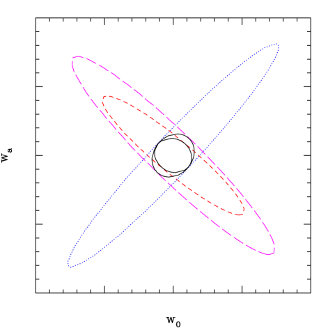
Figure 1: This cartoon illustrates the value of orthogonality in the equation of state plane for tightly constraining dark energy parameters. The short dashed ellipse represents a distance-redshift probe, or any other that has an anticorrelation between the equation of state parameters. Adding a positive correlation probe (dotted) gives a joint contour (inner solid curve) with considerably smaller uncertainties. This also helps to reduce the impact of systematics (long dashed curve and outer solid curve). However the situation is more complicated when marginalizing over a larger set of parameters.

The growth of large scale structure, or equivalently the evolution of gravitational potentials, and hence, say, the number of galaxy clusters of a certain mass, might seem to offer a different dependence than distances. But the growth equation also has $H$ as its predominant ingredient and indeed in hutcoo we see that the growth factor still possesses the anticorrelation. An exception might occur for models where the dark energy (or alternative gravity theory) is inhomogeneous itself and can act as a source to the matter density perturbations, but this is not expected to occur for scalar field dark energy on subhorizon scales caldwell ; dave .

If simple measures of distances or products of distances all give anticorrelation, yet they involve differing levels of sensitivity. This provides the hope that opposing these quantities through ratios might break the pattern of degeneracy. Indeed this was found in linap on consideration of the cosmic shear test originated by alpac . Here the key quantity was $H(z)d_{A}(z)\sim H(z)\int dz/H(z)$, where $d_{A}$ is the angular diameter distance. For a certain redshift range, $z\approx 1.3-2.3$ (for $\Omega_{m}=0.3$), the competition between the two ingredients causes a positive correlation between $w_{0}$ and $w_{a}$. A critical pitfall however was that systematic uncertainties could blow up the constraint contour in a preferred direction such that the resulting contour actually exhibited an anticorrelation (compare Figs. 5 and 8 of linap ). Another indication of positive correlation was found between discrete values of $w(z)$ in neighboring redshift bins by songknox for ratios of distances entering weak gravitational lensing calculations.

Here we investigate distance ratios that appear in strong gravitational lensing measurements. Specifically, we consider $r_{ls}/r_{s}$, related to the angular separation $\Delta\theta$ between multiple images of a source, $r_{ls}/(r_{l}r_{s})$, related to the time delay $\Delta t$ between the images, and $r_{l}r_{ls}/r_{s}$, connected with the length scale of caustic properties, or the cross section, of the lensing. Here $r_{l}$ is the comoving distance to the lens, $r_{s}$ to the source, and $r_{ls}$ between the source and lens; in a flat universe $r_{ls}=r_{s}-r_{l}$.

Figure 2 illustrates the sensitivity of each of these ratios to the cosmological parameters as a function of redshift. We have taken the redshift to represent the lens redshift $z_{l}$ and for convenience fixed the source redshift to be $z_{s}=2z_{l}$ (since that gives roughly the greatest probability of effective lensing). Generally the greatest sensitivity is to the magnitude of the matter (or dark energy) density, then to the present value of the dark energy equation of state ratio, and least to the time variation of the equation of state.

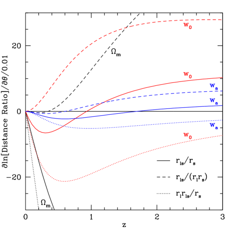
Figure 2: The sensitivity of the distance ratios to the cosmological parameters $\theta=\{\Omega_{m},w_{0},w_{a}\}$ are encoded in the derivatives plotted here, normalized to 1% fractional measurement of the distance ratio. The larger the absolute magnitude of the derivative at a particular redshift, the more constraining the observations there.

Of most interest to our investigation are the crossings from negative to positive sensitivity, i.e. at some redshift the distance ratio switches from diminishing to growing as we change the value of a parameter $\theta=\{\Omega_{m},w_{0},w_{a}\}$ (increasing it, say). Since these crossings occur at different redshifts if the parameter is $w_{0}$ than if it is $w_{a}$, then the correlation between these quantities can shift from negative to positive. We see that positive correlation occurs for $r_{ls}/r_{s}$ for $z_{l}\approx 0.9-1.7$ and for $r_{ls}/(r_{l}r_{s})$ for $z_{l}\approx 0-0.6$; zero crossing in equation of state variables and hence positive correlation does not occur for $r_{l}r_{ls}/r_{s}$. (The exact values will depend on the fiducial cosmology, here taken to be $\Omega_{m}=0.3$, $w_{0}=-1$, $w_{a}=0$.)

For the ratio $r_{ls}/r_{s}$ we expect rapid evolution in the $w_{0}-w_{a}$ degeneracy direction as the contour will rotate from horizontal at $z=0.9$ (no sensitivity to $w_{0}$, so lying parallel to the $w_{0}$-axis) to vertical at $z=1.7$ (no sensitivity to $w_{a}$). Fig. 3 shows this behavior in a “flower” plot, with idealized precision to better illustrate the degeneracy direction. A strong lensing survey measuring image separations from lenses within this redshift range should possess good internal complementarity and the ability to constrain the dark energy equation of state. Furthermore, in this range strong lensing will have near orthogonality with supernova distance and weak gravitational lensing surveys and so be a valuable complementary probe.

Figure 3: Confidence contours for an idealized experiment measuring the ratio $r_{ls}/r_{s}$ rotate depending on the redshift. Degeneracy directions follow the Fisher sensitivities from Fig. 2, with zero crossings of a parameter giving contours parallel to that axis. Note the strong positive correlation between equation of state variables for $z_{l}=1.3$, and hence strong complementarity with, e.g., distance measurements.

The ratio $r_{ls}/(r_{l}r_{s})$ appears somewhat less promising. Its sensitivity to $w_{a}$ is much weaker in the key redshift range and the evolution of the correlation between $w_{0}$ and $w_{a}$ much less dramatic. In particular the contour never tilts far from the vertical. This means it is not as complementary either internally or with other cosmological probes. But it does possess three interesting characteristics: its overall sensitivity to the equation of state is reasonably large at $z>1$, the positive correlation region is at low redshifts where observations are easier (though there is less volume, hence fewer lens systems), and it has an odd null sensitivity with respect to $\Omega_{m}$ at $z=0.35$. This last is where its sensitivity to $w_{a}$ is maximal in the positive correlation region and eases degeneracy with the matter density and hence reduces the need for a tight external prior on it. So time delay measurements should not be wholly neglected as a possibly useful probe.

III Constraints on Cosmological Parameters

So far we have only concentrated on the degeneracy direction. What about the actual magnitude of constraints capable of being imposed on the cosmological parameters? If we consider one parameter $\theta$ at a time, fixing the others, we can obtain a lower limit on the parameter estimation uncertainty. This is given by

$$\delta\theta\geq\left|\frac{\partial[{\rm Distance\ Ratio}]}{\partial\theta}\right|^{-1}\delta[{\rm Distance\ Ratio}].$$ (5)

In Fig. 2 we took a fractional measurement error of 1%. Thus, for example, the sensitivity for $r_{ls}/r_{s}$ with respect to the parameter $w_{0}$ at $z=0.3$ is -6.5 so the best possible estimate of $w_{0}$ from such a single, 1% measurement is 1/6.5=0.15. That is, the unmarginalized uncertainty is $\sigma(w_{0})=0.15$. This will be degraded by degeneracies with other parameters, or by worse precision in the measurement, and improved by additional measurements, subject to some systematics floor.

In fact, degeneracies with additional parameters wash out the simple orthogonality of Fig. 1. The parameter phase space is actually 3-dimensional (from $\Omega_{m}$) or higher and the joint probabilities do not merely trace the intersection of the contours in the equation of state plane. This weakening of apparent complementarity also means that the magnitude of the sensitivity with redshift matters as well as the degree of correlation, and this can alter the favored redshift range. All these effects need to be taken into account.

Here we seek to establish what improvements the complementarity of strong lensing data with other probes such as distance-redshift or weak lensing data can realistically provide. Next generation precision in all three of these come in one package: the proposed Supernova/Acceleration Probe (SNAP: snap ). With some $10^{7}$ galaxies observed in its deep survey (down to AB mag $R=30$) and $10^{8}$ in its wide survey (to AB mag $R=27.5$), the canonical estimate of one strong lens system per thousand galaxies provides an anticipated wealth of data. Other valuable data sets will come from LSST lsst and LOFAR lofar .

III.1 Image Separation

If we consider an optimistic strong lensing measurement precision of 1% in a redshift bin of 0.1, whether through statistical means, e.g. 100 lens systems of 10% precision, or as a systematic floor, we find that the parameter uncertainties are large if we do not a priori fix some of the variables. Even employing the orthogonal combination of measurements of the strong lensing separation variable $S=r_{ls}/r_{s}$ at $z=0.9$ and $z=1.7$ (cf. Fig. 3), the estimations are $\sigma(w_{0})=0.15$, $\sigma(w_{a})=0.53$ even with $\Omega_{m}$ fixed, and 0.28, 0.93 with a prior on $\Omega_{m}$ of 0.03. The lack of sensitivity of the strong lensing separation to the dark energy equation of state and, as mentioned above, the degeneracy with the other parameter, $\Omega_{m}$, prevent as well its complementarity with other probes from being as effective as might have been hoped from §II.

Figure 4 shows contours in the $w_{0}-w_{a}$ plane, now marginalized over $\Omega_{m}$, for various combinations of probes. This considers 1% measurements at $z=0.9$, 1.3, 1.7. The improvements in parameter estimation remain modest: about 15% in $w_{0}$ and $w_{a}$ when added to SNAP supernova distance data, 19% and 3% respectively when added to the supernova plus weak lensing data set, 25% and 13% when added to supernova plus Planck CMB data, and 17% and 6% when added to all three data sets. If strong lensing $S$ measurements were available from $z=0.1-1.7$, say (recall this is the lens redshift, with the source assumed to lie at twice this redshift), the improvement to the triple data set increases to 30% and 15%. If the measurement floor for the strong lensing was instead at 2%, then the constraints in conjunction with the other three probes only gain due to strong lensing by 6% and 2% for $z=0.9$, 1.3, 1.7 or 17% and 7% for $z=0.1-1.7$.

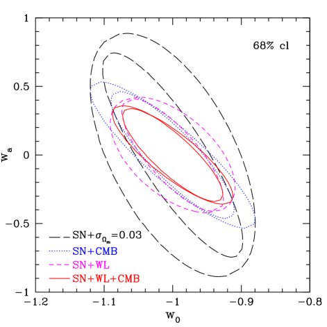
Figure 4: Estimates of the dark energy equation of state parameters from various combinations of cosmological probes (SN=supernovae, WL=weak lensing, CMB=cosmic microwave background) improve modestly with the addition of strong lensing image separation measurements. Outer contours of each pair of line types include the labeled data sets as will be provided by SNAP and Planck; inner contours add the 1% strong lensing constraint.

III.2 Time Delay

The other strong lensing quantity we consider is $T=r_{ls}/(r_{l}r_{s})$, related to the time delay between images. This introduces an extra parameter – the Hubble constant $H_{0}$, which we marginalize over. Again, measurements of strong lensing by itself provide only poor estimates of the cosmological parameters, even for combinations of redshifts where the degeneracy directions are complementary. The insensitivity to $\Omega_{m}$ at low redshift noted in §II does not help since the overall weak dependence and degeneracy of the equation of state variables prevents precision constraints.

In complementarity with supernova distances, strong lensing $T$ measurements of 1% precision at $z=0.1-0.6$ provide improvement by 21% and 9% in $w_{0}$ and $w_{a}$. Adding them to all three other data sets helps by 13% and 9%, or 22% and 15% if the strong lensing measurements extend from $z=0.1-1.7$. Weakening the precision to 2% adjusts this last case to 7% and 5%. Note that no external prior on $H_{0}$ is required; it is determined from the data to better than 1%.

III.3 Image Separation and Time Delay

Simultaneous addition of both separation and time delay information allows further improvements. Relative to the supernova only data, these are 36% and 41% for 1% strong lensing data at $z=0.1,0.3,\dots 1.7$; added to all three other probes they yield tighter constraints by 31% and 17%. With only 2% precision the improvements in the latter case are 15% and 7%. We show the parameter constraints in Fig. 5 for the three probes without strong lensing, with strong lensing for the fiducial redshift bins, for a reduced strong lensing redshift range, and for the weaker 2% strong lensing precision.

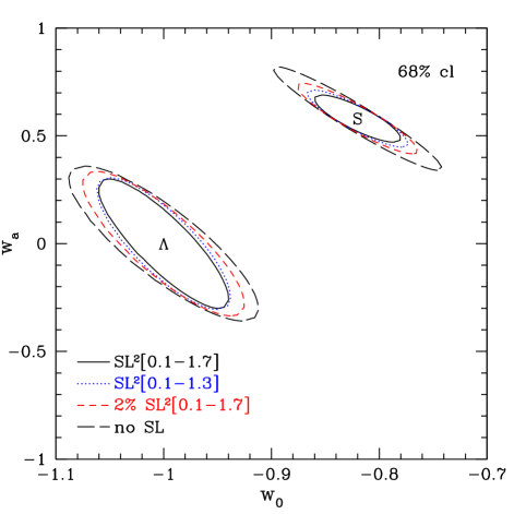
Figure 5: Estimates of the dark energy equation of state parameters from supernovae, weak lensing, and CMB measurements can be further tightened by adding observations of both strong lensing quantities (SL²): image separations and time delays. The outer, long dashed ellipse with no strong lensing and “$\Lambda$” in its center corresponds to the outer solid ellipse of Fig. 4. Strong lensing data at 1% precision adds valuable complementarity (solid ellipse), even over a reduced redshift range (dotted). Higher systematic uncertainties on strong lensing (2%: short dashed), however, strongly diminish its usefulness. As usual (cf. linbo ), dark energy models with time varying equation of state such as the SUGRA model (ellipses centered around “S”) show enhanced complementarity.

The highest redshift bins are not that powerful but it is important to include the $z=0.1$ bin to constrain $H_{0}$, which is strongly degenerate with $w_{0}$ and $w_{a}$. Even with $H_{0}$ known to better than 1% from the data, the degeneracy still plays an important role since the strong lensing time delay probe is so much more sensitive to $H_{0}$ than to the equation of state.

As usual, taking the fiducial cosmology to be that of a cosmological constant tends to underestimate both the sensitivity and complementarity of the probes linbo . For comparison Fig. 5 includes contours for a supergravity inspired dark energy model with time varying equation of state: S(UGRA) with $w_{0}=-0.82$, $w_{a}=0.58$. Here strong lensing offers more dramatic improvements, by 49% in estimating $w_{0}$ and 54% in $w_{a}$ for 1% precision and 29% and 22% for 2% precision. Even at 2% precision the final uncertainty from the four probes in complementarity achieves an impressive constraint on the time variation of $\sigma(w^{\prime})=0.05$.

IV Conclusion

While strong lensing does not completely fulfill the promise of orthogonal constraints on the dark energy equation of state that would provide vastly improved parameter estimates, it does offer some complementarity, especially for models with time varying equation of state. Furthermore, the data resources required will be innate within the deep and wide optical and near infrared surveys of SNAP; abundant strong lensing data should also come from LOFAR at radio wavelengths and both strong and weak lensing from LSST in the optical. We find that strong lensing adds reasonable value to dark energy constraints when the measurements reach the 1% precision level. This is in accord with other calculations (e.g. yamamoto ; lewisibata ). Precision arises from statistics subject to a systematics floor.

The challenge in the next generation will not be the search for sufficient strong lensing data, it will be achieving systematics limits sufficiently low to allow the statistical wealth and the value of strong lensing complementarity to come into play. Currently 1% sounds rather optimistic for a bound to systematic uncertainties. The main contribution is likely to come from our ignorance of the lensing mass model. For example, within a singular isothermal sphere model 1% measurement of the distance ratio $S$ requires knowledge of the velocity dispersion to 0.5% dhk . Cross correlation of different sources with the same lens to remove systematics, à la bernjain for weak lensing, would not work, both because of the rarity of strong lensing and because sources at different distances and positions would probe different parts of the lensing mass distribution.

One might hope to constrain the lensing mass distribution by making use of the simultaneous weak lensing information that SNAP or LSST would provide, but this will be of little use according to dalal . Basically the weak lensing measurements of shears average over a larger range of scales (or multipoles) than the convergence contribution from the mass to the strong lensing. It is like trying to locate a pin with thick gloves. Nongaussian effects also need to be incorporated in a more rigorous treatment of strong lensing. Relaxation of the simplification that sources lie at redshifts $z_{s}=2z_{l}$ is unlikely to change significantly the results shown here.

The advantage of image separations and time delays is that they are well defined and used as markers of the cosmic geometry. One could also use the statistics of lensing systems, e.g. the number of lenses out to some redshift (e.g. sarbu ; oguri ; kuhlen ), but then one must deal with astrophysical scatter and observational bias and incompleteness. Furthermore, lensing counts depend on mass density growth and volume factors that take us further from our original goal of finding orthogonal probes in the equation of state plane.

Since systematics are the limiting factor, we can attempt to seek out special lensing systems that ameliorate these uncertainties, such as strongly lensed calibrated candles (e.g. Type Ia supernovae holz ; ogurik ), time evolving, differentially amplified sources (e.g. Type II supernovae goobar ; wagoner ), or relatively clean Einstein cross or ring images. With the wealth of future data such subsampling may be practical.

While interrelations between cosmological parameters entering into distances and the expansion rate prevent clean orthogonality between cosmological probes, the various methods retain sufficient complementarity to both crosscheck each other and further tighten constraints on the nature of dark energy. If the systematics challenge can be met, in special systems at least, strong lensing merits further consideration in joining the cosmological toolbox of next generation probes.

References

- (1) E.V. Linder and A. Jenkins, MNRAS 346, 573 (2003); astro-ph/0305286
- (2) E.V. Linder, in draft
- (3) J.A. Frieman, D. Huterer, E.V. Linder, M.S. Turner, Phys. Rev. D67, 083505 (2003); astro-ph/0208100
- (4) E.V. Linder, Phys. Rev. D68, 083503 (2003); astro-ph/0212301
- (5) H-J. Seo and D.J. Eisenstein, Ap. J. 598, 720 (2003); astro-ph/0307460
- (6) E.V. Linder, Phys. Rev. D68, 083504 (2003); astro-ph/0304001
- (7) M. Takada and B. Jain, astro-ph/0310125
- (8) S. Majumdar and J.J. Mohr, astro-ph/0305341
- (9) S. Weinberg, Gravitation and Cosmology (Wiley, 1972)
- (10) E.V. Linder, First Principles of Cosmology (Addison-Wesley, 1997)
- (11) R.C. Tolman, Proc. Nat. Acad. Sci. 16, 511 (1930); note the traditional reference is I.M.H. Etherington, Phil. Mag. 15, 761 (1933) but this actually writes the relation with one fewer power of due to a different distance definition.
- (12) E.V. Linder, Astron. Astrophys. 206, 190 (1988)
- (13) B.A. Bassett, astro-ph/0311495
- (14) A. Cooray, D. Huterer and D. Baumann, astro-ph/0304268
- (15) E.V. Linder, Phys. Rev. Lett. 90, 091301 (2003); astro-ph/0208512
- (16) E.V. Linder, in Identification of Dark Matter, ed. N.J.C. Spooner and V. Kudryavtsev (World Scientific, 2003); astro-ph/0210217
- (17) C.P. Ma, R.R. Caldwell, P. Bode, and L. Wang, Ap. J. 521, L1 (1999); astro-ph/9906174
- (18) R. Davé, R.R. Caldwell, and P.J. Steinhardt, Phys. Rev. D66, 023516 (2002); astro-ph/0206372
- (19) C. Alcock and B. Paczyński, Nature 281, 358 (1979)
- (20) Y-S. Song and L. Knox, astro-ph/0312175
- (21) SNAP: http://snap.lbl.gov
- (22) LSST: http://www.noao.edu/lsst
- (23) LOFAR: http://www.lofar.org
- (24) K. Yamamoto, Y. Kadoya, T. Murata, and T. Futamase, Prog. Theor. Phys. 106, 917 (2001); astro-ph/0110595
- (25) G.F. Lewis and R.A. Ibata, MNRAS 337, 26 (2002); astro-ph/0206425
- (26) A.N. Davis, D. Huterer, and L.M. Krauss, MNRAS 344, 1029 (2003); astro-ph/0210494
- (27) G.M. Bernstein and B. Jain, Ap. J. 600, 17 (2004); astro-ph/0309332
- (28) N. Dalal, D.E. Holz, X. Chen, and J.A. Frieman, Ap. J. 585, L11 (2003); astro-ph/0206339
- (29) N. Sarbu, D. Rusin, and C-P. Ma, Ap. J. 561, L147 (2001); astro-ph/0110093
- (30) M. Oguri, Y. Suto, and E.L. Turner, Ap. J. 583, 584 (2003); astro-ph/0210107
- (31) M. Kuhlen, C.R. Keeton, and P. Madau, Ap. J. accepted; astro-ph/0310013
- (32) D.E. Holz, Ap. J. 556, L71 (2001); astro-ph/0104440
- (33) M. Oguri and Y. Kawano, MNRAS 338, L25 (2003); astro-ph/0211499
- (34) A. Goobar, E. Mörtsell, R. Amanullah, and P. Nugent, A&A 393, 25 (2002); astro-ph/0207139
- (35) E.V. Linder, R.V. Wagoner, and P. Schneider, Ap. J. 324, 786 (1988)