Hydrodynamical interaction between an accretion flow and a stellar wind

Abstract

Molecular clouds in the interstellar medium suffer gravitational instabilities that lead to the formation of one or multiple stars. A recently formed star inside a cold cloud communicates its gravitational force to the surrounding environment and soon an accretion flow falling into the star develops. After their formation, all stars soon eject a wind of gas that interacts with the external accretion flow. This interaction produces a shock wave that evolves with time. The work presented in this article formulates a simple prescription for the evolution of this interaction. With the aid of this model we construct a few radio continuum maps of the source.

Keywords: hydrodynamics – shock waves – accretion

$\S$1 Introduction

When a low mass, isolated star is formed inside a gas cloud because of a gravitational collapse, the process of accreting gas from the cloud onto the star begins (Shu et al., 1987). At a later time a wind of gas emanating from the star collides with the accretion flow. Depending on the ram pressure that the wind generates, it will be able to expand forever (when the ram pressure of the wind is much greater than the ram pressure of the medium), reach a steady state (when accretion and wind ram pressures are comparable) or collapse in the surface of the star (when the accretion ram pressure is greater than that of the wind) (Wilkin & Stahler, 1998, 2003).

Bondi (1952) investigated the form of a spherical accretion flow induced by the gravitational pull of a central object. Because of the spherical symmetry of the accretion quantities, the shocks produced by the spherical wind and the accretion flow are both spherical and evolve with time. Ulrich (1976) made modifications to the spherical accretion model by considering a cloud with a small angular momentum. The cloud is rotating about an axis on which the central star lies. The result is that the accretion quantities in this model have cylindrical symmetry, i.e. they do not depend explicitly on the azimuthal angle. The interaction between this “Ulrich flow” and the spherical wind from the star produces two shocks that evolve with time. In this article we develop a simple model for this particular hydrodynamical interaction. We do this by equating the ram pressure of the wind with the ram pressure of the accretion flow. This is the easiest way to model the interaction.

Wilkin & Stahler (2003) have already constructed a numerical solution to the problem by solving the complete hydrodynamical equations. These authors have included on their code not only pressure forces that give rise to the shocks. On their analysis they also included centrifugal forces that appear because of the curvature of the shock, and they took into account the gravitational field produced by the central star. The problem with such a general solution is that it is not very easy to predict observational quantities. In the present article we show how, with a simplified method, it is possible to produce radio continuum maps of the interaction between the wind and the accretion flow.

In section $\S$2 we describe briefly Ulrich’s accretion model. Sections $\S$3 and $\S$4 describe the steady state and the time evolution of the interaction. Finally, in section $\S$5 we describe the validity of the predicted thin layer approximation and we calculate radio continuum maps from our model.

$\S$2 Ulrich’s accretion model

Let us briefly discuss some of the most important properties of a small angular momentum accretion flow that falls to a central compact object, such as a star. This type of accretion flow was first investigated by Ulrich (1976).

Consider a star, or any other compact object of mass $M$. The star is embedded on a gas cloud, which for simplicity will be consider to be of infinite extension. Far away from the star, the density $\rho_{\infty}$, the pressure $p_{\infty}$ and the velocity of sound $c_{\infty}$ have uniform constant values. We assume that the cloud is rotating about the $z$ axis as a solid body in such a way that its specific angular momentum $\Gamma$ has the value $\Gamma_{\infty}$ far away from this axis. We will consider the case in which the accretion process is so low, that the mass $M$ of the central object can be taken as constant. Finally, we assume that the flow has reached a steady state. The accretion flow obeys a polytropic relation

$$\frac{p}{p_{\infty}}=\left(\frac{\rho}{\rho_{\infty}}\right)^{\kappa},$$ (2.1)

where $p$ and $\rho$ are the pressure and density of the gas respectively, and $\kappa$ is the polytropic index.

Due to the fact that the accretion rate $\dot{M}$ in Bondi (1952) accretion flow is constant, and under the assumption that the mass of the central object is much greater than the gas mass contained on a sphere of radius $r$ ($r$ the distance from the star to a certain fluid particle), the self gravity of the gas is negligible with respect to the gravity of the central object. In what follows we will consider $\Gamma_{\infty}$ to be small so that the accretion with rotation can be considered to be a perturbation from the non-rotational accretion Bondi flow.

The problem is characterised by the following parameters: the gravitational constant $G$, the radius of the central object $r_{0}$, the constants $\Gamma_{\infty}$, $M$, $\rho_{\infty}$, $p_{\infty}$, $c_{\infty}$, and the polytropic index $\kappa$. With these quantities it is possible to build three dimensionless parameters (without counting $\kappa$)

$$\delta=\frac{r_{0}c_{\infty}^{2}}{GM},\qquad\epsilon=\left(\frac{\Gamma_{\infty}c_{\infty}}{GM}\right)^{2},$$ (2.2)

and $p_{\infty}/\rho_{\infty}c_{\infty}^{2}\sim 1$. The length $r_{\text{c}}=GM/c_{\infty}^{2}$ is (apart from a function that depends of $\kappa$ which is of order one) the radial distance where the fluid particle reaches the velocity of sound in the accretion without rotation (Bondi, 1952). In other words, the fact that $\delta\ll 1$ ensures that the radius of the central object is small compared with this distance.

The dimensionless parameter $\epsilon$ is ratio of the centrifugal force to the gravitational force of a fluid particle evaluated at position $r_{\text{c}}$. Thus, if we impose the condition $\epsilon\ll 1$, the rotational effects are small perturbations to the Bondi accretion flow.

Due to the fact that the angular momentum of the accretion flow must be conserved, eventually the centrifugal force ($\sim\Gamma^{2}/r^{3}$) will be equal to the gravitational force ($GM/r^{2}$). The position $r_{\text{d}}=\epsilon r_{\text{c}}$ where this occurs is precisely the distance where the flow deviates considerably from the Bondi spherical accretion and where a disc of radius $r_{\text{d}}$ on the equatorial plane forms (Cantó et al., 1995).

Low mass, recently formed stars are such that $r_{0}\sim 2\,\mathrm{R}_{\odot}$, $c_{\infty}\sim 1\,\text{km}\,\text{s}^{-1}$, $M\sim 1\,\textrm{M}_{\odot}$, with an azimuthal velocity far away from the star of the order of $\dot{\varphi}\sim 10^{-14}\textrm{s}^{-1}$, and a lifetime $\tau$ value such that $10^{4}\textrm{yrs}\lesssim\tau\lesssim 10^{5}\textrm{yrs}$. With these values, the angular momentum far away from the rotation axis takes the value $\Gamma_{\infty}=(c\tau)^{2}\dot{\varphi}\sim 9.61\times 10^{18}\,\textrm{cm}^{2}\,\textrm{s}^{-1}$. Thus, for low mass, recently formed stars, it follows that $\delta\sim 1.75\times 10^{-5}\ll 1$, $\epsilon\sim 0.2\ll 1$, $r_{c}\sim 536\,\textrm{AU}$ and $r_{d}\sim 100\,\textrm{AU}$.

At time $\tau=0$, when the gravitational effects produced by the star begin to be noticed by the gas in the cloud, the gas starts to be accreted. In what follows we will consider that the time $\tau$ is sufficiently large so that $\int^{r_{\text{c}}}_{0}\mathrm{d}r/c(r)<\tau$, in which $c(r)$ represents the local sound speed. For instance, if the accretion gas is isothermal, the speed of sound is constant and the previous inequality means that $r_{\text{c}}<c\tau$. For the general case in which the velocity of sound is not constant, this argument implies that the points $r$ contained inside the sphere determined by $\int_{0}^{r}\mathrm{d}r/c(r)>\tau$ are not perturbed by the gravitational effects of the star. On the other hand, the gas particle points $r$ inside the shell that satisfies $\int_{0}^{r_{\text{c}}}\mathrm{d}r/c(r)<\int_{0}^{r}\mathrm{d}r/c(r)<\tau$ are such that they are being accreted to the centre subsonically and its rotational effects are negligible. The flow inside the region $r_{\text{d}}<r<r_{\text{c}}$ is being accreted with a supersonic velocity and its rotational effects are small. When $r<r_{\text{d}}$, the rotational effects are very important on the dynamics of the accretion flow and the velocity of the gas flowing towards the centre is supersonic.

Because pressure gradients and variations on the internal energy along the streamlines of the accretion flow inside the sphere of radius $r_{\text{c}}$ contribute little to the energy and momentum equations, the streamlines can be taken as ballistic. If we also consider that the mass of the disc $M_{\text{d}}$ is much smaller than the mass of the central object, then the trajectory of a fluid element of the accretion flow is described by a central Newtonian potential.

The total mechanical and internal energy of a fluid element far away from the central object is non–zero. This is because the azimuthal component of the velocity and the temperature differ from zero at that point. Nevertheless, the difference between the total energy and the kinetic plus potential energy of a fluid element near the disc is small. This is valid for small values of the rotational kinetic energy (i.e. when $\epsilon\ll 1$) and when heating due to radiation is insignificant. In other words, the streamlines near the disc have to be parabolic trajectories such that

$$E=\frac{1}{2}v^{2}-\frac{GM}{r}\approx 0,$$ (2.3)

where $E$ is the energy per unit mass of a fluid element near the disc and $v$ its velocity. Once the particles reach the plane $\theta=\pi/2$ ($\theta$ the polar angle) where the disc lies, the particles merge into the disc. Because of this, the only interesting trajectories for the accretion flow are the upstream trajectories to the disc.

For simplicity, in what follows we will work with dimensionless quantities, unless stated otherwise. In other words, let us make the changes

$$\frac{r}{r_{d}}\longrightarrow r\ ,\qquad\frac{v_{i}}{v_{\text{k}}}\longrightarrow v_{i},\quad\left(i=r\ ,\theta,\varphi\right)\qquad\frac{\rho}{\rho_{0}}\longrightarrow\rho,$$ (2.4)

where the natural velocity $v_{\text{k}}$ and density $\rho_{0}$ are defined by

$$v_{\text{k}}=\left(\frac{GM}{r_{d}}\right)^{1/2},\qquad\rho_{0}=\frac{\dot{M}}{4\pi r_{d}^{2}v_{\text{k}}}.$$ (2.5)

The analytical form of the stream lines, the velocity field and density for the accretion flow with rotation are given by (Ulrich, 1976)

$$r=\frac{\sin^{2}\theta_{0}}{1-\cos\theta/\cos\theta_{0}},$$ (2.6)

$$v_{r}=-\left(\frac{1}{r}\right)^{1/2}\left(1+\frac{\cos\theta}{\cos\theta_{0}}\right)^{1/2},$$ (2.7)

$$v_{\theta}=\left(\frac{1}{r}\right)^{1/2}\frac{\cos\theta_{0}-\cos\theta}{\sin\theta}\left(1+\frac{\cos\theta}{\cos\theta_{0}}\right)^{1/2},$$ (2.8)

$$v_{\varphi}=\left(\frac{1}{r}\right)^{1/2}\left(1-\frac{\cos\theta}{\cos\theta_{0}}\right)^{1/2}\frac{\sin\theta_{0}}{\sin\theta},$$ (2.9)

$$\rho=r^{-3/2}\left(1+\frac{\cos\theta}{\cos\theta_{0}}\right)^{-1/2}\left\{1+2r^{-1}P_{2}\left(\cos\theta_{0}\right)\right\}^{-1},$$ (2.10)

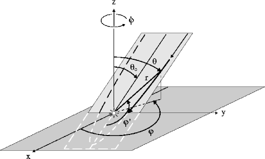
Figure 1: Far away from the star, the fluid particles in Ulrich’s accretion rotate like a solid body with constant angular velocity $\dot{\varphi}$. These particles follow parabolic trajectories near the central object (star). Only upstream trajectories to the equatorial plane are of interest.

where $v_{i}$ ($i=r,\theta,\varphi$), and $\rho$ are the velocity and density fields of the accretion flow respectively. The azimuthal angle is represented by $\varphi$. The initial polar angle $\theta_{0}$ that a fluid element has once it begins its way down towards the disc (see Figure 1), $\dot{M}$ is the accretion rate and $P_{2}\left(\xi\right)$ is the second order Legendre polynomial given by

$$P_{2}\left(\xi\right)=\frac{1}{2}\left(3\xi^{2}-1\right).$$ (2.11)

A plot of the streamlines (Eq. (2.6)) projected on a plane $\varphi=\text{const}$ is shown in Figure 2. The angle $\theta_{0}$ labels a particular streamline. For each $\theta_{0}$ there is only one streamline, because they cannot intersect. It is clear from the velocity field equations that when $\theta_{0}\rightarrow 0$, the polar and azimuthal components of the velocity become zero as well. Thus, the streamlines become parallel near the axis of rotation.

The velocity and density field equations are functions that depend only on the particle’s position and not of the initial polar angle $\theta_{0}$. This is easily seen by rewriting Eq. (2.3) as

$$\cos^{3}\theta_{0}+\cos\theta_{0}(r-1)-r\cos\theta=0,$$ (2.12)

which has a solution (see appendix Appendix)

$$\cos\theta_{0}=\begin{cases}\left(\cos\theta\right)^{1/3},\\ \qquad\qquad\thickspace\text{for }r=1,\\ 2\left(\frac{r-1}{3}\right)^{1/2}\sinh\left\{\frac{1}{3}\textrm{arcsinh}\left(\frac{r\cos\theta}{2\left(\frac{r-1}{3}\right)^{3/2}}\right)\right\},\\ \qquad\qquad\thickspace\text{for }r>1,\\ 2\left(\frac{1-r}{3}\right)^{1/2}\cosh\left\{\frac{1}{3}\textrm{arccosh}\left(\frac{r\cos\theta}{2\left(\frac{1-r}{3}\right)^{3/2}}\right)\right\},\\ \qquad\qquad\thickspace\text{for }r<1\text{ and }\left(\frac{r\cos\theta}{2}\right)^{2}-\left(\frac{1-r}{3}\right)^{3}>0,\\ 2\left(\frac{1-r}{3}\right)^{1/2}\cos\left\{\frac{1}{3}\textrm{arccos}\left(\frac{r\cos\theta}{2\left(\frac{1-r}{3}\right)^{3/2}}\right)\right\},\\ \qquad\qquad\thickspace\text{for }r<1\text{ and }\left(\frac{r\ \cos\theta}{2}\right)^{2}-\left(\frac{1-r}{3}\right)^{3}<0.\end{cases}$$ (2.13)

Thus, Eqs. (2.7)-(2.10) and Eq. (2.13) provide the velocity and density fields as functions of the polar angle $\theta$ and the radial coordinate $r$ only.

From Eq. (2.12) it is easy to see that

$$\cos\theta_{0}\bigg{|}_{\theta=\frac{\pi}{2}}=\Theta\left(1-r\right)\sqrt{1-r},$$ (2.14)

$$\cos{\theta_{0}}=1-\frac{\theta^{2}}{2}\left(\frac{r}{r+2}\right),\quad\text{ as }\theta\rightarrow 0,$$ (2.15)

where $\Theta(\chi)$ is the Heaviside step function with a value of $1$ for $\chi>0$ and $0$ for $\chi<0$. With the substitution of Eq. (2.14) and Eq. (2.15) into Eq. (2.10) it is possible to give values for the density in the equatorial plane and the polar axis respectively

$$\rho\left(\theta=\pi/2\right)=\begin{cases}\frac{1}{2}r^{-1/2}\left(1-r\right)^{-1},&\text{for }r<1,\\ \left(2r-1\right)^{-1/2}\left(r-1\right)^{-1},&\text{for }r\geq 1,\end{cases}$$ (2.16)

$$\rho\left(\theta=0\right)=\left(2r\right)^{-1/2}\left(r+2\right)^{-1}.$$ (2.17)

The fact that the density tends to infinity as $r$ tends to zero for any $\theta$ is due to the accumulation of the accreted gas around the central object. Nevertheless, the border of the disc (i.e. $r=1$ and $\theta=\pi/2$) has also an infinite density. This is because we are considering an infinitely thin disc and so, border effects on it are expected to appear.

Figure 3 shows the variation of the density as a function of position for different polar angles. This plot, together with the density contours (as shown by Figure 4) can be used to make a detailed analysis of the density distribution in the accretion flow.

$\S$3 Steady interaction

From now on, let us suppose that the central object is a recently formed star, and that a supersonic, spherical wind with constant radial velocity is being produced by it. In this section we discuss the interaction between the Ulrich accretion flow described in Section $\S$2 with the wind of the star.

The interaction between the supersonic accretion flow and the supersonic stellar wind gives rise to an initial discontinuity. The end result of this interaction is the production of two shock waves and a tangential discontinuity between both. In the frame of reference of the tangential discontinuity, the shocks separate from each other. Under the assumption that both shocks occupy the same position in space, so that we can call both shocks “the shock” for simplicity, we analyse the geometrical form that the shock has under the assumption that the only type of forces that keep the shock stable are pressure forces. Apart from pressure forces, there will be centrifugal forces (produced by the post–shock material) acting on the walls of the shocks. These forces are originated because the shock is curved. In section $\S$5 we analyse under which conditions, the assumption that both shocks occupy the same position in space (thin layer approximation) is valid by studying the cooling lengths of the flow. It turns out that for the steady case, this approximation is correct.

Under these assumptions, the locus of the points of the shock are given by balancing the ram pressure produced by both flows, the accretion flow and the stellar wind. In other words, the shock is located at points for which

$$\rho_{\text{w}}v_{\text{wn}}^{2}=\rho v_{\text{n}}^{2},$$ (3.1)

where the subindex w labels quantities related to the stellar wind and $n$ means the normal component of the velocity. The wind’s density is determined by the mass loss rate $\dot{M}_{\text{w}}$ of the star

$$\dot{M}_{\text{w}}=4\pi r^{2}v_{\text{w}}\rho_{\text{w}}.$$ (3.2)

In order to get a dimensionless form of Eq. (3.1), we make the changes

$$\frac{v_{\text{wn}}}{v_{\text{w}}}\longrightarrow v_{\text{wn}},\qquad\frac{\rho_{\text{w}}}{\rho_{\text{w}0}}\longrightarrow\rho_{\text{w}},$$ (3.3)

where $\rho_{\text{w0}}=\dot{M}_{\text{w}}/4\pi r_{\text{d}}^{2}v_{\text{w}}$. Combining these changes with the ones presented in Eq. (2.4) we obtain

$$\rho_{\text{w}}v^{2}_{\text{wn}}\lambda=\rho v^{2}_{\text{n}}$$ (3.4)

where $\lambda$ is a dimensionless parameter given by

$$\lambda\equiv\frac{\dot{M}_{\text{w}}v_{\text{w}}}{\dot{M}v_{\text{k}}}.$$ (3.5)

Eq.(3.4) determines the position $\boldsymbol{r}(\theta,\varphi)$ of the shock as a function of the polar angle $\theta$ and the azimuthal angle $\varphi$. A normal vector to this surface is given by

$$\boldsymbol{n}=\frac{\partial\boldsymbol{r}}{\partial\theta}\times\frac{\partial\boldsymbol{r}}{\partial\varphi},$$ (3.6)

since $\partial\boldsymbol{r}/\partial\theta$ and $\partial\boldsymbol{r}/\partial\varphi$ are tangent vectors to any surface parametrised by the polar and azimuthal angles. Because the accretion flow and the stellar wind have azimuthal symmetry, the shock wave position should not depend on the angle $\varphi$. Since the length element $\mathrm{d}\boldsymbol{r}=\mathrm{d}r\boldsymbol{e}_{r}+r\mathrm{d}\theta\boldsymbol{e}_{\theta}+r\sin\theta\mathrm{d}\varphi\boldsymbol{e}_{\varphi}$, where $\boldsymbol{e}_{i}$ ($i=r,\theta,\varphi$) are unitary vectors in the i–th direction, then Eq. (3.6) can be rewritten in the following form

$$\widehat{\boldsymbol{n}}=\frac{r\boldsymbol{e}_{r}-\left(\partial r/\partial\theta\right)\boldsymbol{e}_{\theta}}{{\left\{r^{2}+\left(\partial r/\partial\theta\right)^{2}\right\}}^{1/2}},$$ (3.7)

where $\widehat{\boldsymbol{n}}\equiv\boldsymbol{n}/n$ is a unit vector in the direction of $\boldsymbol{n}$.

The accretion flow and wind velocities are radial on the rotation axis. This means that the locus of the shock satisfies the following boundary condition

$$\frac{\partial r}{\partial\theta}\bigg{|}_{\theta=0}=0.$$ (3.8)

Using Eq. (3.7) and Eq. (3.8), it follows from Eq. (3.4) that over the rotation axis of the cloud, the value of the distance $r$ from the star to the shock is given by

$$r\bigg{|}_{\theta=0}=-2+\frac{1-\sqrt{1-4\lambda^{2}}}{\lambda^{2}}.$$ (3.9)

This equation implies that for $\lambda>1/2$ there is no value for the initial condition of the position of the shock. In other words, there is no steady solution for the case when $\lambda>1/2$.

The equation satisfied by the spatial points on the shock $r(\theta)$ is given by substitution of Eq. (3.6) into Eq. (3.4), that is

$$\frac{\partial r}{\partial\theta}=\frac{\lambda^{1/2}+\rho^{1/2}rv_{r}}{\rho^{1/2}v_{\theta}}.$$ (3.10)

Figure 5 shows integrals of Eq. (3.10) for different values of the parameter $\lambda$. These integrals were obtained with a 4th rank Runge–Kutta method. From the figure it follows that when $\lambda\leq 1/2$ the shocks can be classified in two cases. Those that have positive derivatives with respect to the polar angle ($\lambda=0.2$, for example) and those for which this derivative is negative ($\lambda=0.48$, for example). Let us show that there is no configuration for which this derivative is zero for all polar angles. For this, it is sufficient to assume that the configuration is a circumference. It then follows that $r(\theta=0)=r(\theta=\pi/2)$. From this and Eq. (3.9) it follows that the obtained value for $\lambda$ does not correspond to a circle.

Until now, we have considered that both shocks, the accretion shock and the wind shock, occupy the same position in space. However, as shown by the cartoon of Figure 6, there is an intermediate region of shocked gas between them. Let us calculate the direction that the post–shocks should have immediately after crossing their corresponding shocks. Under the assumption that both shocks are highly radiative, the post–shock normal velocities are negligible. Nevertheless, since the tangential components of the velocity are continuous through the shock, the post–shock direction is determined by the tangential components of the pre–shock velocity. Because the shock is not a function of the azimuthal angle, a unitary tangent vector to it’s surface is given by

$$\widehat{\boldsymbol{\tau}}=\frac{\left(\partial r/\partial\theta\right)\boldsymbol{e}_{r}+r\boldsymbol{e}_{\theta}}{{\left\{r^{2}+\left(\partial r/\partial\theta\right)^{2}\right\}}^{1/2}}.$$ (3.11)

Due to the symmetry of the problem, it is useful to analyse only the region $0\leq\theta\leq\pi/2$. Using the tangent vector of Eq. (3.11) and because the polar component of the velocity is positive for the accretion flow, we say that the post–shock flow (either accretion or stellar wind) “goes up” if $\boldsymbol{v}\cdot\hat{\boldsymbol{\tau}}<0$ (i.e., the flow leaves the equatorial plane) and the flow “goes down” if $\boldsymbol{v}\cdot\hat{\boldsymbol{\tau}}>0$ (i.e., the flow approaches the equatorial plane). Figure 7 shows values of the pre–shock tangential velocities for both flows as a function of the polar angle for different values of the parameter $\lambda$. From this figure it follows that in the case of the stellar wind, for $\lambda\lesssim 0.3$ the post–shock flow goes down and for $\lambda\gtrsim 0.3$ this post–shock flow goes up. When $\lambda\approx 0.3$ the post–shock flow goes up in some regions and goes down in some others. For the accretion flow, the situation is different. It always goes down, regardless of the configuration chosen. It is important to note that there is an accumulation point of material, corresponding to the polar axis ($\theta=0$). In this point, both post–shock flows have no motion. In this accumulation point, it is expected that the post–shock flow collimates to regions away from the star when the centrifugal forces are taken into account.

$\S$4 Time evolution

Let us now analyse the evolution in time of the interaction between the stellar wind and the accretion flow. As discussed in section $\S$3, two shocks are formed. For simplicity we will consider that both shocks occupy the same position in space and we will refer to this region as the shock, unless stated otherwise. If we assumme that only ram pressure forces act on the surface of the shock, then from the system of reference of the shock Eq. (3.1) is also valid. In order to transform it to the frame of reference of the star, we make the transformation

$$v_{\text{wn}}\longrightarrow\left(v_{\text{wn}}-v_{\text{sn}}\right),\qquad v_{\text{n}}\longrightarrow\left(v_{\text{sn}}-v_{\text{n}}\right),$$ (4.1)

where $v_{\text{wn}},\ v_{\text{sn}},\ v_{\text{n}}$ represent the velocities of the stellar wind, the shock wave and the accretion flow respectively, all normal to the shock wave. With these changes, Eq. (3.1) gives

$$\rho_{\text{w}}\left(v_{\text{wn}}-v_{\text{sn}}\right)^{2}=\rho\left(v_{\text{sn}}-v_{\text{n}}\right)^{2}.$$ (4.2)

In order to write Eq. (4.2) in a dimensionless form, we use the changes described in Eq. (2.4) and Eq. (3.3) together with

$$\frac{v_{\text{sn}}}{v_{\text{k}}}\longrightarrow v_{\text{sn}}.$$ (4.3)

Performing these transformations, Eq. (4.2) can be written as

$$v_{\text{sn}}=\frac{\left(\lambda\rho_{\text{w}}\right)^{1/2}v_{\text{wn}}+v_{\text{n}}\rho^{1/2}}{\left(\eta\rho_{\text{w}}\right)^{1/2}+\rho^{1/2}},$$ (4.4)

where $\lambda$ is defined by Eq. (3.5) and $\eta$ is another dimensionless parameter given by

$$\eta\equiv{\lambda}{\left(\frac{v_{\text{k}}}{v_{\text{w}}}\right)^{2}}.$$ (4.5)

When $v_{\text{sn}}\rightarrow 0$, that is when the evolutionary shock becomes steady, Eq. (4.4) converges to Eq. (3.4).

Since we are only interested in the geometrical shape of the shock and not on the particular trajectory that a small fragment of the shock follows, we analyse only the form that the shock will have as a function of time for a fixed polar angle. Because of this, the relation between the shock’s radial velocity $v_{\text{s}}$ and its normal velocity can be obtained from Eq. (3.7)

$$v_{\text{sn}}=\frac{rv_{\text{s}}}{\left\{r^{2}+\left(\partial r/\partial\theta\right)^{2}\right\}^{1/2}}.$$ (4.6)

With this, Eq. (4.4) can be rewritten as

$$v_{\text{s}}=\frac{\partial r}{\partial t}=\frac{\left(\lambda\rho_{\text{w}}\right)^{1/2}r+\rho^{1/2}\left\{rv_{\text{r}}-v_{\theta}\partial r/\partial\theta\right\}}{r\left\{\left(\eta\rho_{\text{w}}\right)^{1/2}+\rho^{1/2}\right\}},$$ (4.7)

where the normal values of the stellar wind and the accretion flow given by Eq. (3.7) have been used.

Near the star, for $r\ll 1$, the velocity field and density for the accretion flow are spherically symmetric and coincide with the spherical symmetry of these quantities for the stellar wind. In other words, at time $t=0$ the shock is a spherical surface of radius $r_{\star}$, the radius of the star

$$r\left(\theta,t=0\right)=\frac{r_{0}}{r_{\text{d}}}\ll 1.$$ (4.8)

Since Eq. (4.4) has two dimensionless parameters, we will consider in what follows that the star is a recently formed star of low mass. For these stars (Black & Matthews, 1985) $v_{\text{w}}\sim 300\,\textrm{km}\,\textrm{s}^{-1}$, $M\sim 1M\odot$ y $r_{\text{d}}\sim 100\,\textrm{au}$. With these values, the parameter $\eta$ can be determined uniquely by the values of $\lambda$ through the following expression

$$\eta=10^{-4}\lambda.$$ (4.9)

The solution of Eq. (4.7) with the initial condition given by Eq. (4.8) was obtained by numerical integration using MaCormack & Paullay (1972) corrector method. The integrals for this equation are plotted in Figure 8. The solutions show that the steady state is only reached for $\lambda\leq 1/2$, and so there is a convergence of these solutions to the ones obtained in the previous section. When $\lambda>1/2$ the shock grows indefinitely, apart from the equatorial plane, where the shock reaches the border of the disc and stays there for sufficiently large times (see the case $\lambda=0.7$ of Figure 8 for example). This effect is due to the infinite value that the accretion density reaches in the border of the disc.

Using Eqs. (2.6)-(2.10) for $r\gg 1$ and Eq. (4.7) it is possible to obtain the relation that the shock surface must have for sufficiently large times

$${\frac{\partial r}{\partial t}}={\frac{2^{1/4}\lambda^{1/2}}{r^{1/4}}},\quad\text{ as }r\rightarrow\infty,$$ (4.10)

which has a solution

$$r=\left(\frac{5\lambda^{1/2}}{2^{7/4}}\right)^{4/5}t^{4/5}.$$ (4.11)

Figure 9 shows for which times the approximation made with Eq. (4.11) is valid on the polar axis of the shock.

$\S$5 Astrophysical consequences

We have assumed that the shock produced by the stellar wind, as well as the one produced by the accretion flow, occupy the same position in space. In this section we analyse under which circumstances this approximation is correct. As usual, we define the cooling length $l_{\text{c}}$ as the distance travelled by a particle from the shock front until it reaches a point in which the temperature has a value $\sim 10^{4}\,\textrm{K}$ (Hartigan et al., 1987).

Hartigan et al. (1987) estimated cooling lengths for different shock velocities $v_{\text{sn}}$ in the interval $20\textrm{ km }\textrm{s}^{-1}\lesssim v_{\text{sn}}\lesssim 400\textrm{ km }\textrm{s}^{-1}$, and particle number density $n$ in the interval $100\textrm{ cm }^{-3}\lesssim n\lesssim 1000\textrm{ cm }^{-3}$. From their results it follows that (Cantó et al., 1988)

$$\left(\frac{l_{\text{c}}}{\textrm{AU}}\right)=A\left(\frac{v_{\text{sn}}}{100\textrm{km}\textrm{s}^{-1}}\right)^{\beta}\left(\frac{n}{\textrm{cm}^{-3}}\right)^{-1},$$ (5.1)

where

$$A=\begin{cases}6.6&v_{\text{sn}}\lesssim 70\textrm{km}\textrm{s}^{-1},\\ 43.33&v_{\text{sn}}\gtrsim 70\textrm{km}\textrm{s}^{-1}.\end{cases}$$ (5.2)

and

$$\beta=\begin{cases}-5.5&v_{\text{sn}}\lesssim 70\textrm{km}\textrm{s}^{-1},\\ 5.7&v_{\text{sn}}\gtrsim 70\textrm{km}\textrm{s}^{-1}\end{cases}$$ (5.3)

From now on, we will assume that Eq. (5.1) is valid for any density and velocity ranges.

The equations that describe the accretion flow (Eqs. (2.6)-(2.10)), the stellar wind flow (Eq. (3.4)), the shock velocity (Eq. (4.4)) and the time can be written in dimensional form as follows

$$r=r_{\text{d}}\widetilde{r},\quad\rho=\rho_{0}\widetilde{\rho},\quad v_{\text{i}}=v_{\text{k}}\widetilde{v}_{\text{i}}\ \ \text{(}i=r,\theta,\varphi\text{)},\quad v_{\text{s}}=v_{\text{k}}\widetilde{v}_{\text{s}},$$

$$v_{\text{w}}=v_{\text{w}}\widetilde{v}_{\text{w}},\quad\rho_{\text{w}}=\rho_{\text{w}0}\widetilde{\rho}_{\text{w}},\quad t=\left(r_{\text{d}}/v_{\text{k}}\right)\widetilde{t},$$ (5.4)

where tilded quantities are referred to the dimensionless variables considered in the previous sections. We now give values of the hydrodynamical quantities for the accretion flow and the stellar wind for typical values of recently formed stars of low mass

$$\left(\frac{v_{\text{k}}}{\textrm{km}\ \textrm{s}^{-1}}\right)=3\left(\frac{M}{M_{\odot}}\right)^{1/2}\left(\frac{r_{\text{d}}}{100\textrm{AU }}\right)^{-1/2},$$ (5.5)

$$\begin{split}\left(\frac{n_{0}}{\textrm{cm}^{-3}}\right)=3.6\times 10^{6}&\left(\frac{\dot{M}}{10^{-6}\textrm{M}_{\odot}\text{yr}^{-1}}\right)\times\\ &\times\left(\frac{r_{\text{d}}}{100\textrm{AU }}\right)^{-3/2}\left(\frac{M}{\textrm{M}_{\odot}}\right)^{-1},\end{split}$$ (5.6)

$$\begin{split}\left(\frac{n_{\text{w}0}}{\textrm{cm}^{-3}}\right)=3\times 10^{4}&\left(\frac{\dot{M}_{\text{w}}}{10^{-7}}{\textrm{M}_{\odot}\text{yr}^{-1}}\right)\times\\ &\times\left(\frac{r_{\text{d}}}{100\textrm{ AU }}\right)^{-2}\left(\frac{v_{\text{w}}}{300\textrm{km}\ \textrm{s}^{-1}}\right)^{-1},\end{split}$$ (5.7)

where $n_{0}$ y $n_{\text{w}0}$ are the particle number densities of the accretion flow and the stellar wind respectively with the assumption that the average mass per particle is $\bar{m}\sim 1.3m_{H}$. As shown by Eq. (5.5), typical values of the velocity $v_{\text{k}}$ are sufficiently small to be used in the calculation of the cooling length of the accretion flow using Eq. (5.1). Thus, from now on, we will only analyse the cooling lengths for the stellar wind.

In order to simplify things further we calculate the cooling lengths for the stellar wind leaving fixed the quantities $M$, $\dot{M}$, $r_{d}$, $v_{\text{w}}$, with typical values as the ones showed in Eqs. (5.5)–(5.7) and we will only vary the quantity $\dot{M}_{\text{w}}$. Table 5.1 shows the maximum variation of the ratio of the cooling length to the length between the shocks for different polar angles in the steady case. These results show that, for the steady case the assumption of a thin post–shock layer is correct for the stellar wind.

$\lambda$	$\left(l_{\text{c}}/r\right)_{\text{max}}\times 10^{3}$
0.04	0.54
0.08	1.08
0.12	1.65
0.16	2.25
0.20	2.88
0.24	3.56
0.28	4.27
0.32	5.20
0.36	6.38
0.40	7.96
0.44	10.35
0.48	15.21

Table 5.1: Values of the cooling length in the steady case for the shock produced by the stellar wind as a function of the parameter $\lambda$. The quantity $(l_{c}/r)_{\text{max}}$ represents the maximum value of the ratio of the cooling lengths $l_{c}$ to the position of the shock $r$, for different polar angles.

Let us now analyse the cooling lengths of the stellar wind for the case in which the shock evolves with time. In the frame of reference of the shock wave, the formulae used for the steady case are valid. With the aid of Eq. (4.1), in the frame of reference of the central star, Eq. (5.1) takes the following form

$$\left(\frac{l_{\text{c}}}{\textrm{AU}}\right)=A\left(\frac{\widetilde{v}_{\text{wn}}v_{\text{w}}-\widetilde{v}_{\text{sn}}v_{\text{k}}}{100\textrm{km}\textrm{s}^{-1}}\right)^{\beta}\left(\frac{\widetilde{\rho}_{\text{w}}n_{\text{w}0}}{\textrm{cm}^{-3}}\right)^{-1}.$$ (5.8)

In this case, it follows that the ratio of the cooling length to the radial distance to the star, when $\lambda>1/2$, is large. To see this, let us make an asymptotic expansion of Eq. (5.8) for $r\gg 1$. With this, and using Eq. (4.11), it is found that

$$\left(\frac{l_{\text{c}}}{\textrm{ AU }}\right)\left(\frac{\widetilde{r}r_{\text{d}}}{\textrm{ AU }}\right)^{-1}=A\left(\frac{5\lambda^{1/2}}{2^{7/4}}\right)^{4/5}\left(\frac{v_{\text{w}}}{100\textrm{km}\textrm{s}^{-1}}\right)^{\beta}\times\left(\frac{n_{\text{w}0}}{{\textrm{cm}^{-3}}}\right)^{-1}\left(\frac{r_{\text{d}}}{\textrm{ AU }}\right)^{-1}\widetilde{t}^{4/5},$$ (5.9)

as $t\rightarrow\infty$. Figure 10 shows at which times the thin layer approximation ends its validity for certain values of the parameter $\lambda>1/2$. In the case where the shock evolves with time, for $\lambda\leq 1/2$, the cooling lengths and the distance to the shock are always small until the steady configuration is obtained, converging to the values shown on Table 5.1.

Let us now analyse the shape that a radio continuum observation will show of the interaction described so far. For this, we assume that the shock emission is due to free–free processes and we use the brightness temperature $T_{\text{B}}$ given by

$$T_{B}=T\left(1-e^{-\tau_{\nu}}\right),$$ (5.10)

where $T$ is the temperature produced by the shocks. The optical depth $\tau_{\nu}$ in the continuum, at a radio frequency $\nu$ of a shock wave with velocity $v_{\text{s}}$ and a pre–shock density $n$ is given by (Curiel et al., 1989)

$$\begin{split}\tau_{\nu}=9.83\times 10^{-7}&\left(\frac{n}{\textrm{cm}^{-3}}\right)\left(\frac{v_{s}}{300\textrm{km}\textrm{s}^{-1}}\right)^{1.68}\times\\ &\times\left(\frac{T}{10^{4}\textrm{K}}\right)^{-0.55}\left(\frac{\nu}{5\textrm{ GHz }}\right)^{-2.1}.\end{split}$$ (5.11)

For our model, it follows that $\tau_{\nu}\ll 1$ and so, Eq. (5.10) can be written as

$${T_{B}}=T\tau_{\nu},\quad\text{ as }\tau_{\nu}\rightarrow 0.$$ (5.12)

Figures 11-12 show different projections of the brightness temperature isocontours on the plane of the sky for typical values of $\dot{M}_{w}=10^{-7}\textrm{M}_{\odot}\textrm{yr}^{-1}$ ($\lambda=10$).

Let us now calculate the emission flux produced by the stellar wind shock for the value used in Figures 11-12 in which $\dot{M}_{\text{w}}=10^{-7}\textrm{M}_{\odot}\textrm{yr}^{-1}$ $(\lambda=10)$. For this case, the emission flux received on the plane of the sky is given by (Rodríguez, 1990)

$$S_{\nu}=\frac{2kT\nu^{2}}{\mathrm{c}^{2}}\int{\mathrm{d}\Omega\tau_{\nu o}},$$ (5.13)

where the integral is extended over the solid angle $\Omega$ occupied by the shock surface on the plane of the sky and $\mathrm{c}$ is the speed of light. The optical depth $\tau_{\nu 0}$ is observed through the plane of the sky. The quantity $\tau_{\nu 0}d\Omega=\tau_{\nu}\mathrm{d}a/D^{2}$, where $\mathrm{d}a$ is the area element and $\tau_{\nu}$ is the optical depth, both normal to the shock surface. With this and because $D$ is the distance from the observer to the shock surface, Eq. (5.13) can be rewritten as

$$S_{\nu}=\frac{2KT\nu^{2}}{D^{2}\mathrm{c}^{2}}\int{\mathrm{d}a\tau_{\nu}}.$$ (5.14)

Using Eq. (3.7) in spherical coordinates, Eq. (5.14) takes the form

$$S_{\nu}=\frac{2KT\nu^{2}}{D^{2}\mathrm{c}^{2}}\oint{\frac{\mathrm{d}\theta\mathrm{d}\varphi\tau_{\nu}r\sin\theta}{\sqrt{r^{2}+{\left(\partial r/\partial\theta\right)^{2}}}}\left\{r^{2}-\left(\partial r/\partial\theta\right)^{2}\right\}}.$$ (5.15)

In our case, Eq. (5.15) is

$$\left(\frac{S_{\nu}}{\textrm{mJy}}\right)=0.406\left(\frac{T}{10^{4}\textrm{K}}\right)\left(\frac{\nu}{5\textrm{ GHz }}\right)^{2}\left(\frac{D}{150\textrm{ pc }}\right)^{-2}\Phi,$$ (5.16)

where

$$\Phi\equiv\int^{\pi/2}_{0}{\frac{\mathrm{d}\theta\tau_{\nu}r\sin\theta}{\sqrt{r^{2}+\left(\partial r/\partial\theta\right)^{2}}}\left\{r^{2}-\left(\partial r/\partial\theta\right)^{2}\right\}},$$ (5.17)

and $r$ is measured in astronomical units.

When $\lambda>1/2$, because the derivative of the shock with respect to the polar angle vanishes for sufficiently large times, the emission flow tends to a constant value given by

$$\begin{split}\left(\frac{S_{\nu}}{\textrm{mJy}}\right)=3.37&\left(\frac{\dot{M}_{\text{w}}}{10^{-7}}{\textrm{M}_{\odot}\text{yr}^{-1}}\right)\left(\frac{v_{\text{w}}}{300\textrm{km}\textrm{s}^{-1}}\right)^{1.68}\times\\ &\times\left(\frac{T}{10^{4}}{\textrm{K}}\right)^{2}\left(\frac{\nu}{5\textrm{GHz}}\right)^{-0.1}\left(\frac{D}{150\textrm{ pc }}\right)^{-2},\quad\text{ as }t\rightarrow\infty.\end{split}$$ (5.18)

Figure 13 shows the emission flux as a function of time for $\dot{M}_{\text{w}}=10^{-7}\textrm{M}_{\odot}\textrm{yr}^{-1}$ $(\lambda=10)$.

$\S$6 Conclusions

We have developed a simple prescription to describe the hydrodynamical interaction between a rotating accretion flow onto a star with a spherically symmetric wind. For simplicity we considered a purely hydrodynamical flow, with no magnetic fields. The evolution of the shock wave produced by the interaction of the wind with the accretion flow is thus described by balancing the wind’s force $\sim\dot{M}_{\text{w}}v_{\text{w}}$ with the accretion flow’s force $\sim\dot{M}v_{\text{k}}$, where $v_{\text{k}}$ is the keplerian velocity that a particle has at a characteristic distance of $r_{\text{d}}$, the radius of the disc. That allowed us to define a dimensionless parameter $\lambda$ given by Eq. (3.5). For very large values of $\lambda$, the surface of interaction expands to infinity and the thin layer approximation breaks down. For small values of $\lambda$, in fact for $\lambda<1/2$, it is possible to reach a steady configuration.

We would like to point out that a full analysis of the interaction should take into account the gravitational pull that the central star makes on the gas and the equilibrium equation must also include a centrifugal term. If magnetic fields are to be included on the whole description of the problem as well, then magnetic pressure will also play an important role on the structure of the cavities. We will make a more precise analysis considering all these physical processes in a future article.

Appendix

Eq.(2.12) is a reduced Cardan third order algebraic equation, i.e.

$$x^{3}\pm 3\alpha x+2\beta=0,$$ (A1)

with

$$\alpha=|\frac{r-1}{3}|,\qquad\beta=-\frac{r\cos\theta}{2},\quad\text{and}\quad x=\cos\theta_{0}.$$ (A2)

The solutions of Eq. (A2) are given by (Namias, 1984)

$$x=\begin{cases}2\alpha^{1/2}\sinh\left\{\frac{1}{3}\textrm{arcsinh}\left(-\beta/\alpha^{3/2}\right)\right\},\\ \qquad\qquad\qquad\qquad\text{for a }+\text{ sign},\\ 2\alpha^{1/2}\cosh\left\{\frac{1}{3}\text{arccosh}\left(-\beta/\alpha^{3/2}\right)\right\},\\ \qquad\qquad\qquad\qquad\text{for a }-\text{ sign and }\beta^{2}-\alpha^{3}>0,\\ 2\alpha^{1/2}\cos\left\{\frac{1}{3}\arccos\left(-\beta/\alpha^{3/2}\right)\right\},\\ \qquad\qquad\qquad\qquad\text{for a }-\text{ sign \& }\beta^{2}-\alpha^{3}<0.\end{cases}$$ (A3)

For each case in Eq. (A3) there exist three different solutions due to the fact that

$$\arccos z=\pm\arccos_{\text{p}}z+2k\pi,$$

$$\text{arcsinh}z=(-)^{k}\text{arcsinh}_{\text{p}}z+2k\pi i,$$

$$\text{arccosh}z=\pm\text{arccosh}_{\text{p}}z+2k\pi i,$$ (A4)

with $k=0,\;\pm 1,\;\pm 2,\ldots$ The subindex p refers to the main Riemann sheet.

For our particular case, we are interested in real solutions, so for the second and third cases in Eq. (A4) we set $k=0$. For the first case, due to the symmetry of the problem, we consider only values of the polar angle such that $0\leq\theta\leq\pi/2$. Let us define $\mu\equiv-\beta/\alpha^{3/2}$ and analyse the behaviour of the function $\zeta=\cos\left\{(\arccos\mu)/3+2k\pi\right\}$ with $k=0,\ \pm 1$. When $\mu>0$ we expect $\zeta\geq 0$. Since $\zeta(\mu\geq 0,\,k=0)>0$ then the required solution occurs when $k=0$. In other words, the required full solution is given by Eq. (A3) with $k=0$.

Figure 2: The figure shows the streamlines of the accretion flow with rotation projected on a plane with constant azimuthal angle. Every single streamline is labelled by its initial polar angle $\theta_{0}$, which is the initial particle’s angle with respect to the $Z$ axis as the gas begins to be accreted to the star. Lengths in the diagram are measured in units of the radius of the disc $r_{\text{d}}$.

Figure 3: Accretion density $\rho$ varies continuously from $\theta=0$ to $\theta=\pi/2$. The density tends to infinity in the point $r=1$ for the $\theta=\pi/2$ curve which corresponds to the border of the disc. $R$ represents the cylindrical radius ($R\equiv r\sin\theta$). Lengths are measured in units of the radius of the disc ($r_{d}$) and the density is measured in units of $\rho_{0}$ (see text). The polar angle $\theta^{\prime}$ is such that $\theta=(\pi/60)\theta^{\prime}$.

Figure 4: Density isocontours are shown as continuous lines for the accretion flow. The density $\rho$ is measured in units of the density $\rho_{0}$. Lengths are measured in units of the radius of the disc. Different numbers in the plot represent different values of the density.

Figure 5: The interaction between the stellar wind and the accretion flow produces two strong shock waves. It is assumed that both shocks occupy the same position in space. $R$ represents the cylindrical radius ($R\equiv r\sin\theta$), and $Z$ is the polar axis coordinate. Distances are measured in units of the radius of the disc $r_{\text{d}}$.

Figure 6: The interaction between the stellar wind and the accretion flow forms two shock cavities. The figure shows a schematic representation of this interaction with both shocks lying close to each other. The arrows in the figure show the direction of the flow velocity immediately after crossing the shocks. The cylindrical radius $R$ and the polar coordinate $Z$ are both measured in units of the accretion disc radius $r_{\text{d}}$.

Figure 7: The post–shock direction is given by the values of the pre–shock tangential velocity values for each flow. The tangential velocity of the stellar wind $v_{\text{w}\tau}$ is measured in units of the wind’s velocity $v_{\text{w}}$. The accretion velocity $v_{\tau}$ is measured in units of the velocity $v_{\text{k}}$ The numbers on the plot are values of the quantity $\lambda^{\prime}$ defined by $\lambda=0.05\lambda^{\prime}$.

Figure 8: The figure shows the shape of the shock for different time intervals $t$, in units of $r_{\text{d}}/v_{\text{k}}$ and different values of $\lambda$. The shock converges to the steady case of Figure 5 when $\lambda\leq 1/2$ and for sufficiently large values of time $t$. When $\lambda>1/2$ there is no steady configuration and the shock grows indefinitely. The cylindrical radius $R$ and the coordinate $Z$ are measured in units of the radius of the disc $r_{\text{d}}$.

Figure 9: When $\lambda>1/2$, the geometrical form of the shock is spherical for sufficiently large times and its radial coordinate grows as a power law (see Eq. (4.11)). The curves on the plot show the shock position $r$ evaluated on the polar axis measured in units of the radius of the disc $r_{\text{d}}$. Continuous lines show the numerical calculation and dotted ones represent the analytical approximation. The time $t$ is measured in units of $r_{\text{d}}/v_{\text{k}}$.

Figure 10: When the parameter $\lambda>1/2$, the thin layer approximation is no longer valid for sufficiently large times. The plot shows the variation of the cooling length $(l_{c})$ as a function of time. The coordinate $r$ is the distance from the star to the shock. Dotted lines correspond to the asymptotic approximation obtained in Eq. (5.9) and continuous lines correspond to the numerical calculation. The time $t$ is measured in years.

Figure 11: Emission isocontours normalised to the maximum (shown with crosses). The isocontours take values $0.1,\,0.2,\,\ldots 1.0$ with $\dot{M}_{w}=10^{-7}\textrm{M}_{\odot}\textrm{yr}^{-1}$ ($\lambda=10$) and a resolution $\theta_{B}=0^{\prime\prime}.2$ at a distance of $150\textrm{pc}$. The angle $\phi$ is formed between the equatorial plane and the observer. The time $t$ is measured in years. The cylindrical radius $R$ and the coordinate $Z$ are measured in astronomical units.

Figure 12: Emission isocontour variations due to different resolutions, normalised to the maximum (shown with crosses). The isocontours take values $0.1,\,0.2,\,\ldots 1.0$ with $\dot{M}_{\text{w}}=10^{-7}\textrm{M}_{\odot}\textrm{yr}^{-1}$ $(\lambda=10)$ and $t=3197$ yrs. The angle $\phi$ is measured is the angle formed by the equatorial plane and the line of sight. The angle $\theta_{\text{B}}$ represents the resolution. The cylindrical radius $R$ and the coordinate $Z$ are measured in astronomical units.

Figure 13: When the dimensionless parameter $\lambda>1/2$, the emission flux $S$ tends to a constant value for $t\gg 1$. The continuous line represents the numerical calculation and the dotted line the asymptotic analytical value. The time $t$ is measured in years and the flux $S$ in $mJy$.

References

- Black & Matthews (1985) Black, D. C. & Matthews, M. S., eds., 1985. Protostars and planets II.
- Bondi (1952) Bondi, H., 1952. On spherically symmetrical accretion. MNRAS, 112, 195+.
- Cantó et al. (1995) Cantó, J., D’Alessio, P. & Lizano, S., 1995. The Temperature Distribution of Circumstellar Disks. In Revista Mexicana de Astronomia y Astrofisica Conference Series, vol. 1, 217+.
- Cantó et al. (1988) Cantó, J., Tenorio-Tagle, G. & Rozyczka, M., 1988. The formation of interstellar jets by the convergence of supersonic conical flows. Astronomy and Astrophysics, 192, 287–294.
- Curiel et al. (1989) Curiel, S., Rodríguez, L. F., Bohigas, J., Roth, M. & Cantó, J., 1989. Extended radio continuum emission associated with V645 CYG and MWC 1080. Astrophysics Letters, 27, 299–309.
- Hartigan et al. (1987) Hartigan, P., Raymond, J. & Hartmann, L., 1987. Radiative bow shock models of Herbig-Haro objects. ApJ, 316, 323–348.
- MaCormack & Paullay (1972) MaCormack, R. & Paullay, A., 1972. On spherically symmetrical accretion. AIAA Journal, 72, 154+.
- Namias (1984) Namias, V., 1984. Simple derivation of the roots of a cubic equation. Am. J. Phys., 53, 775.
- Rodríguez (1990) Rodríguez, L., 1990. Radio Astronomy lecture notes. IAUNAM.
- Shu et al. (1987) Shu, F., Adams, F. & Lizano, S., 1987. Ann. Rev. Ast. & Ast., 25, 23.
- Ulrich (1976) Ulrich, R. K., 1976. An infall model for the T Tauri phenomenon. ApJ, 210, 377–391.
- Wilkin & Stahler (1998) Wilkin, F. & Stahler, S., 1998. The confinement and breakout of protostellar winds: quasi-steady solution. ApJ, 502, 661–675.
- Wilkin & Stahler (2003) Wilkin, F. & Stahler, S., 2003. Trapped Protostellar Winds and their Breakout. ApJ, 502, 661–675.