Simulations of planet-disc interactions using Smoothed Particle Hydrodynamics

We have performed Smoothed Particle Hydrodynamics (SPH) simulations to study the time evolution of one and two protoplanets embedded in a protoplanetary accretion disc. We investigate accretion and migration rates of a single protoplanet depending on several parameters of the protoplanetary disc, mainly viscosity and scale height. Additionally, we consider the influence of a second protoplanet in a long time simulation and examine the migration of the two planets in the disc, especially the growth of eccentricity and chaotic behaviour. One aim of this work is to establish the feasibility of SPH for such calculations considering that usually only grid-based methods are adopted. To resolve shocks and to prevent particle penetration, we introduce a new approach for an artificial viscosity, which consists of an additional artificial bulk viscosity term in the SPH-representation of the Navier-Stokes equation. This allows accurate treatment of the physical kinematic viscosity to describe the shear, without the use of artificial shear viscosity.

1 Introduction

Since the discovery of the first extrasolar planet in the mid-nineties of the last century by Mayor & Queloz (1995), the interest in planet formation research has grown rapidly. By now about 120 extrasolar planets are known. For comprehensive reviews on extrasolar planets and their detection we refer to Perryman (2000) and Marcy et al. (2000). These newly discovered planetary systems partially feature attributes that differ enormously from those of our solar system. In particular, orbital semi-major axes of down to $2.25\times 10^{-3}$ AU, masses in the range of $0.12-13.75$ M_jup, and large eccentricities of up to $0.927$ have been found, in contrast to the planets in the solar system which orbit the sun at larger distances on almost circular orbits with rather lower masses. Therefore, nowadays planet formation theory not only has to explain the formation of our solar system, but the formation of planetary systems with these substantially different features as well.

It is generally believed that planet formation is part of star formation. Stars are formed by gravitational collapse of a molecular cloud. During this process, angular momentum conservation leads to the formation of a circumstellar disc around a central object, the protostar. The material in the disc slowly accretes onto the protostar in the centre until the protostar becomes a star. Circumstellar discs composed of dust and gas have been found around young T Tauri stars (Beckwith & Sargent 1996). Star formation theory suggests a typical lifetime of such circumstellar discs in the range of $10^{6}$ to $10^{7}$ yr, which determines the time frame for planet formation (see Kallenbach et al. (2000) and references therein). It is assumed that planets form in these circumstellar (or protoplanetary) discs. Two mechanisms are proposed, either fast formation by direct fragmentation due to gravitational instabilities (Mayer et al. 2002; Boss 2001, 2003), or slow formation during a process of several steps: at first the dust in the disc grows via a so-called hit-and-stick mechanism and settles in the mid-plane of the disc, where a dense layer forms (Beckwith et al. 2000). There the solid material is able to combine into larger bodies, which eventually form planetesimals. Finally, planetary-sized objects develop out of these planetesimals by collisions (Ohtsuki et al. 2002). The latter, slower scenario leads to a longer formation time. Calculations by Pollack et al. (1996) suggest a formation time of $1$ to $10$ million years for Jupiter and Saturn, and of $2$ to $16$ million years for Uranus, respectively.

This scenario leads to essentially circular orbits of the planets as they form in a keplerian disc. Due to the lack of material in the inner regions of the disc, more massive planets can only be created at larger distances to the central object. However, while these properties fit well to our solar system where the eccentricities are rather small and the massive planets are located in the outer regions, the model cannot explain the appearance of highly massive planets on significantly eccentric orbits at orbital radii down to $0.04$ AU, as found among the extrasolar planets.

A possible solution to this problem is planet migration. It is generally assumed that these planets have formed further out in the disc and have migrated inwards later. This migration has its cause in tidal interactions of the planet with the disc (Goldreich & Tremaine 1980). The planet exerts tidal torques on the disc which lead to the formation of spiral density wave perturbations. Simultaneously, since the disc loses its axisymmetry, a net torque acts on the planet itself, which starts migrating in radial direction (Lin et al. 2000). The migration rate depends on different factors, such as the mass of the planet, the density distribution in the disc and the viscosity of the disc material.

Another problem lies in the high masses of the discovered planets. The tidal interaction of the planet can eventually lead to the opening of a gap at the planet’s orbital region in the disc, which has a severe impact on the accretion rate. Until the numerical calculations by Artymowicz & Lubow (1996), who modelled the accretion on circumbinaries, and the simulations of a jovian protoplanet embedded in a disc by Kley (1999); Bryden et al. (1999), it has been assumed that accretion stops after gap formation. These simulations however yield a final non-vanishing accretion rate which depends on the viscosity in the disc. Since then, further work has been done on this by various other authors (Lubow et al. 1999; Bryden et al. 2000; Lin et al. 2000; Terquem et al. 2000; Nelson et al. 2000).

While the numerical method known as Smoothed Particle Hydrodynamics (SPH) has been used for one of the first simulations that examined the system of an embedded protoplanet in a disc (Sekiya et al. 1987), later simulations were nearly exclusively performed with grid-based methods, mainly because computer resources have not been available for other high resolution simulations. This has changed only recently. In this paper we present a feasibility study for the simulation of planet-disc interactions with SPH, applying a new approach for the artificial viscosity, and we show the results of simulations with one and two embedded protoplanets in a viscous accretion disc. Very recently, also Lufkin et al. (2004) have used SPH for investigating planet-disc interaction. However, they focus on the scenario where planets form due to selfgravitating instabilities, while we consider non-selfgravitating discs in two dimensions ($r-\varphi$).

The outline of the paper is as follows. In the next section we present the physical model of the system, including an overview on gap formation and planet migration theory. Numerical issues will be discussed in Sect. 3, where especially the approach for a new artificial bulk viscosity will be described. The results of several simulations will be given in 4, followed by a discussion in Sect. 5. Finally, we draw our conclusions in Sect. 6.

2 Physical model

We only consider a non-selfgravitating, thin accretion disc model for the protoplanetary disc. The disc is located in the $z=0$ plane, rotating around the $z$-axis. The vertical thickness $H$ of the disc is assumed to be small in comparison to the radial extension $r$, $H/r\ll 1$. Therefore it is possible to vertically integrate the hydrodynamic equations and use vertically averaged quantities only, neglecting the vertical motion in the disc. The protostar in the centre of the disc always is assumed to have a mass of $M_{\mathrm{c}}=1\mathrm{M}_{\sun{}}$.

2.1 Basic equations

The equations describing a viscid flow of gas in the disc are the continuity equation and the Navier-Stokes equation. In the Lagrangian scheme the former reads

$$\frac{\mathrm{d}\Sigma}{\mathrm{d}t}+\Sigma\@vec{\nabla v}=0,$$ (1)

where $\Sigma$ is the surface density and $\@vec{v}$ the velocity. The surface density is defined by

$$\Sigma=\int_{-\infty}^{\infty}\varrho\mathrm{d}z,$$ (2)

where $\varrho$ denotes the density. The Navier-Stokes equation in Lagrangian formulation reads

$$\frac{\mathrm{d}\@vec{v}}{\mathrm{d}t}=-\frac{1}{\Sigma}\@vec{\nabla}p+\@vec{f}+\frac{1}{\Sigma}\@vec{\nabla}\@tens{T},$$ (3)

where $p$ is the vertically integrated pressure, and $\@vec{f}$ denotes a specific external force, i.e., the gravitational acceleration due to the star and the $N_{\mathrm{p}}$ planets with masses $m_{i}$ and locations $\@vec{r_{i}}$

$$\@vec{f}=-GM_{\mathrm{c}}\frac{\@vec{r}-\@vec{r}_{\mathrm{c}}}{(\@vec{r}-\@vec{r}_{\mathrm{c}})^{3}}-\sum_{i=1}^{N_{\mathrm{p}}}Gm_{i}\frac{\@vec{r}-\@vec{r}_{i}}{(\@vec{r}-\@vec{r}_{i})^{3}}.$$ (4)

The last term in the equation of motion describes the viscous forces and contains the viscous stress tensor which can be written as

$$\@tens{T}_{\alpha\beta} = \eta\left(\frac{\partial v_{\beta}}{\partial x_{\alpha}}+\frac{\partial v_{\alpha}}{\partial x_{\beta}}-\frac{2}{3}\delta_{\alpha\beta}\frac{\partial v_{\gamma}}{\partial x_{\gamma}}\right)+\zeta\delta_{\alpha\beta}\frac{\partial v_{\gamma}}{\partial x_{\gamma}}$$ (5)

$$\equiv \eta\sigma_{\alpha\beta}+\zeta\delta_{\alpha\beta}\frac{\partial v_{\gamma}}{\partial x_{\gamma}},$$ (6)

(Greek indices denote spatial coordinates, and Einstein’s summing convention holds throughout), where the coefficients of shear viscosity, $\eta$, and bulk viscosity, $\zeta$, are positive and do not depend on the velocity.

2.2 Equation of state

For computational simplicity we follow the usual approach and use an isothermal equation of state, where the vertically integrated pressure $p$ is related to the surface density $\Sigma$ by

$$p=c_{\mathrm{s}}^{2}\Sigma.$$ (7)

Here the local isothermal sound speed is given by

$$c_{\mathrm{s}}=\frac{H}{r}v_{\mathrm{kep}},$$ (8)

where $v_{\mathrm{kep}}$ denotes the Keplerian velocity of the unperturbed disc. The scale height of the disc, which is defined as the ratio of the vertical height to the radial distance, $H/r$, equals the inverse Mach number ${\cal M}$ of the flow in the disc and is taken as an input parameter for our disc model. By choosing such an equation of state we suppose that the disc stays geometrically thin and emits all thermal energy which results from tidal and viscous dissipation locally.

2.3 Viscosity

Viscous processes are of great importance in the theory of accretion discs. In order to move radially inwards, the disc material has to lose its angular momentum. Therefore a permanent flow of angular momentum radially outwards and of mass radially inwards takes place in the disc. Often, theories of protostellar discs assume viscous accretions discs, see e.g. Papaloizou et al. (1999). We follow the prescription by Shakura & Sunyaev (1973) and assume an effective $\alpha$-viscosity, where the kinematic viscosity $\nu$ in the disc is given by

$$\nu=\alpha c_{\mathrm{s}}H.$$ (9)

The shear viscosity $\eta$ is related to the kinematic viscosity by $\eta=\nu\Sigma$. Typical $\alpha$-values for protostellar discs are in the range of $10^{-2}$ to $10^{-3}$.

2.4 Gap formation and planet migration

Using perturbation theory, the tidal interaction of the planet and the accretion disc can be analyzed analytically if the planetary mass is much smaller than the mass of the central object, see Goldreich & Tremaine (1979, 1980) for details. The planet exerts torques on the disc material (and vice versa), which can lead to gap opening at the planet’s orbital region if these tidal torques exceed the internal viscous torques in the disc (Papaloizou & Lin 1984). The faster (slower) moving disc material inside (outside) the planet’s orbit exerts a positive (negative) torque on the planet. The planet will begin to migrate radially as soon as these torques do not cancel out. There are two different timescales for migration depending on whether a gap has formed or not, which are called type I and type II migration respectively (Ward 1997).

Type I migration.

No gap formation occurs as long as the response of the disc to the tidal perturbation stays linear. The radial migration velocity of the planet is then given by (Nelson et al. 2000)

$$\frac{\mathrm{d}r}{\mathrm{d}t}\sim-c_{1}q\left(\frac{\Sigma r^{2}}{M_{\mathrm{c}}}\right)\left(r\Omega_{\mathrm{kep}}\right)\left(\frac{r}{H}\right)^{3},$$ (10)

where $q$ denotes the mass ratio of the planet to the central star, $M_{\mathrm{c}}$ the mass of the central star, and $\Omega_{\mathrm{kep}}$ the Keplerian angular velocity. The factor $c_{1}$ accounts for the imbalance of the torques between the two regions of the disc inside and outside the planet’s orbit. Hence, the radial migration velocity will be larger for a more massive planet as long as the response of the disc stays linear.

As soon as the planet has grown to a sufficient high mass, the response of the disc to the perturbation becomes non-linear, and gap formation occurs.

Type II migration.

In order to form a gap the tidal torques exerted by the planet have to exceed the internal viscous torques in the disc. The conditions for gap formation have been widely studied in detail by Papaloizou & Lin (1984), Lin & Papaloizou (1985, 1993), Bryden et al. (1999) and Nelson et al. (2000). Here we only present the different truncation conditions and scenarios for type II migration. A sufficient condition for viscous truncation is

$$q>\frac{40\nu}{\omega r^{2}},$$ (11)

where $\omega$ is the angular velocity of the planet and $r$ its orbital radius. For discs with a very low viscosity Korycansky & Papaloizou (1996) suggest the thermal truncation condition

$$q>\left(\frac{H}{r}\right)^{3}.$$ (12)

During type II migration, the migration of the planet is driven by the viscous evolution of the disc. The migration rate in this case is given by the radial drift velocity of the gas in the disc due to viscous processes (Papaloizou & Lin 1984)

$$\frac{\mathrm{d}r}{\mathrm{d}t}\sim\frac{3\nu}{2r}.$$ (13)

This relation holds as long as the mass of the planet is lower than the mass of the disc material with which it interacts. Otherwise the inertia of the planet gets important and slows down the orbital evolution. This has been studied in detail by Syer & Clarke (1995) and Ivanov et al. (1999). Nelson et al. (2000) find a migration rate based on a model by Ivanov et al. (1999) which reads

$$\frac{\mathrm{d}r}{\mathrm{d}t}\sim\frac{3\nu}{2}\left(10\pi^{4}\Sigma^{4}\right)^{1/5}m_{\mathrm{p}}^{-4/5}r^{3/5},$$ (14)

where $m_{\mathrm{p}}$ is the mass of the planet.

3 Numerical issues

We apply Smoothed Particle Hydrodynamics (SPH) for our simulations. SPH is a grid-free Lagrangian particle method for solving the system of hydrodynamic equations for compressible and viscous fluids first introduced by Gingold & Monaghan (1977) and Lucy (1977). SPH is especially suited for boundary-free problems with high density contrasts. Rather than being solved on a grid, the equations are solved at the positions of the so-called particles, each of which represents a volume of the fluid with its physical quantities like mass, density, temperature, etc. and moves with the flow according to the equations of motion. For a more detailed description see, e.g., Benz (1990) and Monaghan (1992).

3.1 The code

Our SPH-code is fully parallelized to make optimal use of today’s supercomputers which is necessary to achieve the required resolution and accuracy. The parallel implementation is done with the so called ParaSPH Library, a generalized set of routines to simplify and optimize the development of parallel particle codes (Bubeck et al. 1999). This library allows a clear separation between the implementation of the physical problem to be simulated and the parallelization. A programmer using the library works with parallel arrays containing the physical quantities of the SPH-particles and iterators to step through the particles and their neighbours. Domain decomposition, load balancing, nearest neighbour search and communication is hidden in the library. ParaSPH uses MPI (Message Passing Interface) for the communication and works on every parallel architecture providing an MPI library. On a Cray T3E one can achieve a parallel speedup of about 120 using 256 nodes for a problem with 360 000 particles. On the Beowulf-Cluster where we have performed the majority of our simulations – a Pentium III based Linux-Cluster with a Myrinet communication network located at the University of Tübingen – the parallel speedup is about 60 on 128 processors.

3.2 Physical and artificial viscosity, XSPH

To model the physical shear viscosity we use the implementation introduced by Flebbe et al. (1994) and solve the Navier-Stokes equation including the entire viscous stress tensor (6), in contrast to the usual approach of a scalar artificial viscosity term. For the physical shear flow, we assume a constant kinematic viscosity $\nu$ and a vanishing bulk viscosity $\zeta=0$. Then, the acceleration due to the shear stress tensor $\sigma_{\alpha\beta}$ reads

$$\left.\frac{\mathrm{d}v_{\alpha}}{\mathrm{d}t}\right|_{\mbox{shear}}=\frac{1}{\Sigma}\frac{\partial(\nu\Sigma\sigma_{\alpha\beta})}{\partial x_{\beta}}.$$ (15)

Applying the smoothing discretization scheme to the derivative of the stress tensor yields the SPH representation

$$\left.\frac{\mathrm{d}v_{\alpha i}}{\mathrm{d}t}\right|_{\mbox{shear}}=\sum_{j}\frac{m_{j}}{\Sigma_{i}\Sigma_{j}}\left(\nu_{i}\Sigma_{i}\sigma_{\alpha\beta i}+\nu_{j}\Sigma_{j}\sigma_{\alpha\beta j}\right)\frac{\partial W_{ij}}{\partial x_{\beta}}$$ (16)

with the particle form of the shear tensor

$$\sigma_{\alpha\beta i}=V_{\alpha\beta i}+V_{\beta\alpha i}-\frac{2}{3}\delta_{\alpha\beta}V_{\gamma\gamma i},$$ (17)

where $V_{\alpha\beta i}$ is the particle representation of the velocity gradient $\partial v_{\alpha}/\partial x_{\beta}$

$$V_{\alpha\beta i}=\frac{\partial v_{\alpha i}}{\partial x_{\beta}}=\sum_{j}\frac{m_{j}}{\Sigma_{j}}(v_{\alpha j}-v_{\alpha i})\frac{\partial W_{ij}}{\partial x_{\beta}}.$$ (18)

The indices $i$ and $j$ denote quantities that are assigned to SPH particles with positions $\@vec{r}_{i}$ and $\@vec{r}_{j}$, respectively; $m_{j}$ is the particle mass, and $W$ is the usual SPH kernel function. Replacing surface density $\Sigma$ by (volume) density $\varrho$, this SPH-representation of the shear viscosity also holds in 3D.

In order to prevent the particles from mutual penetration, we add an additional artificial bulk viscosity to the viscous stress tensor. The bulk part of the viscous stress tensor is given by $\zeta\@vec{\nabla}\@vec{v}$ and leads to an additional acceleration of particle $i$ according to

$$\left.\frac{\mathrm{d}\@vec{v_{i}}}{\mathrm{d}t}\right|_{\mbox{bulk}}=\sum_{j}m_{j}\zeta_{ij}\frac{(\@vec{\nabla}\@vec{v})_{i}+(\@vec{\nabla}\@vec{v})_{j}}{\Sigma_{i}\Sigma_{j}}\@vec{\nabla}W_{ij}.$$ (19)

The artificial bulk viscosity coefficient for the interaction of particles $i$ and $j$ is given by

$$\zeta_{ij}=\left\{\begin{array}[]{ll}-f\overline{h}_{ij}^{2}(\overline{\@vec{\nabla}\@vec{v}})_{ij}\overline{\Sigma}_{ij}&\quad\mbox{for }\@vec{v}_{ij}\@vec{r}_{ij}<0\\ 0&\quad\mbox{else}\end{array}\right.,$$ (20)

where $h_{i}$ ($h_{j}$) is the smoothing length of particle $i$ ($j$), $\overline{Q}_{ij}$ is an abbreviation for the average $(Q_{i}+Q_{j})/2$ for any quantity $Q$, and the notation $\@vec{v}_{ij}\@vec{r}_{ij}=(\@vec{v}_{i}-\@vec{v}_{j})\cdot(\@vec{r}_{i}-\@vec{r}_{j})$ has been used. Only approaching particles are contributing to the artificial viscosity. The factor $f$ is of order unity and set to $0.5$ in our simulations. The divergence of the velocity is calculated according to

$$(\@vec{\nabla}\@vec{v})_{i}=\frac{1}{\Sigma_{i}}\sum_{j}m_{j}(\@vec{v}_{i}-\@vec{v}_{j})\@vec{\nabla}W_{ij}.$$ (21)

To avoid mutual particle penetration, we additionally use the XSPH-algorithm. The particles are moved at averaged velocity of their interaction partners (Monaghan 1989)

$$\frac{\mathrm{d}\@vec{r_{i}}}{\mathrm{d}t}=\@vec{v}_{i}+x\sum_{j}\frac{2m_{j}}{\Sigma_{i}+\Sigma_{j}}(\@vec{v}_{i}-\@vec{v}_{j})W_{ij},$$ (22)

where $x$ is in the range between 0 and 1. The use of this averaged velocity keeps the particles in their relative local order.

In appendix A we demonstrate the low intrinsic numerical shear stress of this new artificial bulk viscosity approach.

3.3 Migration

To study the migration of the protoplanet in detail, the equation of motion of the protoplanet is integrated. The planet’s acceleration due to the gravitational forces reads

$$\frac{\mathrm{d}\@vec{v}_{\mathrm{p}}}{\mathrm{d}t}=GM_{\mathrm{c}}\frac{\@vec{r}_{\mathrm{p}}-\@vec{r}_{\mathrm{c}}}{\left|\@vec{r}_{\mathrm{p}}-\@vec{r}_{\mathrm{c}}\right|^{3}}+\sum_{i=1}^{N}Gm_{i}\frac{\@vec{r}_{\mathrm{p}}-\@vec{r}_{i}}{\left(\left|\@vec{r}_{\mathrm{p}}-\@vec{r}_{i}\right|^{2}+\delta^{2}\right)^{3/2}}$$ (23)

where $M_{\mathrm{c}}$ is the mass of the central object, $\@vec{r_{\mathrm{c}}}$ its position, $N$ the total number of SPH particles in the simulation with positions $\@vec{r_{i}}$, and $G$ the gravitational constant. Only particles which are not inside the Roche lobe of the planet contribute to the sum. Additionally, the gravitational forces of the particles on the planet are softened by the use of $\delta^{2}$, which is small. The Roche lobe is approximated using the formula by Eggleton (1983)

$$r_{\mathrm{roche}}=\frac{0.49q^{2/3}}{0.6q^{2/3}+\ln(1+q^{1/3})}r_{\mathrm{p}}.$$ (24)

In the case of more than one planet, the additional gravitational forces of the other objects are added to Eq. (23), nevertheless this approximation formula for the Roche lobe is used.

3.4 Initial conditions

The initial setup of our standard model places a jovian planet with mass $m_{\mathrm{p}}=1$ M_jup at $r_{\mathrm{p}}=5.2$ AU and a central object with mass $M_{\mathrm{c}}=1$ M_☉, which gives a mass ratio of $q=9.55\times 10^{-4}$. The surface density $\Sigma$ falls off as $r^{-3/4}$, and the particles with equal masses are distributed according to this density between $r_{\mathrm{min}}=1$ AU and $r_{\mathrm{max}}=10$ AU. The mass of the disc is set to $10^{-2}$ $\mathrm{M_{\sun{}}}$ and the initial particle velocities are $v_{r}=0$ and $v_{\varphi}=v_{\mathrm{kep}}=\sqrt{GM_{\mathrm{c}}/r_{i}}$ as in the unperturbed case. The typical number of particles at the beginning of the simulation is $3\times 10^{5}$. The standard model uses a Mach number of ${\cal M}=20$, that is a scale height $H/r=0.05$, and the kinematic viscosity parameter $\nu_{0}$ is set to $10^{15}$ $\mathrm{cm^{2}/s}$, which corresponds to an $\alpha$ value of about $4\times 10^{-3}$ at the orbital radius of the planet.

As the density falls off with radius, fewer particles are located in the outer regions of the disc than near the central object. Hence, a constant number of interaction partners is more suited to the problem than a fixed smoothing length. Unless otherwise mentioned the number of interaction partners per particle is set to $100$. As mentioned above, we use the XSPH-method to avoid mutual particle penetration and we set $x=0.5$ in all our simulations.

4 Results

In this section we present the results of the simulations with various input parameters. First we consider the case of a single planet in the disc. Afterwards, the case of two planets and their mutual interactions is investigated.

4.1 One planet

4.1.1 Gap formation

In order to study the formation of a gap, we have performed several simulations of a disc with an embedded protoplanet. The disc scale height and the kinematic viscosity have been used as input parameters and have been varied accordingly. Here, the gravitational forces of the particles on the planet have not been considered, keeping it on a circular orbit around the central star. Moreover, the planet was assumed to be able to accrete material without growing in mass, its Roche lobe has been kept constant throughout the simulations.

Just after the start of the simulation the planet disturbs the density distribution in the disc effectively, which leads to the typical spiral density wave pattern in the disc which can be seen in Fig. 1, where a greyscale plot of the surface density is presented for the system after 10 orbits of the protoplanet. In the case of this reference model, gap formation begins immediately after the start of the simulation run. After ten orbits of the planet the decrease of the density at the protoplanet’s orbital region is already clearly visible. The evolution of the azimuthally averaged surface density during the gap formation process is shown in Fig. 2. After one hundred orbits of the protoplanet, the decrease of density at the orbital region is more than two orders in magnitude.

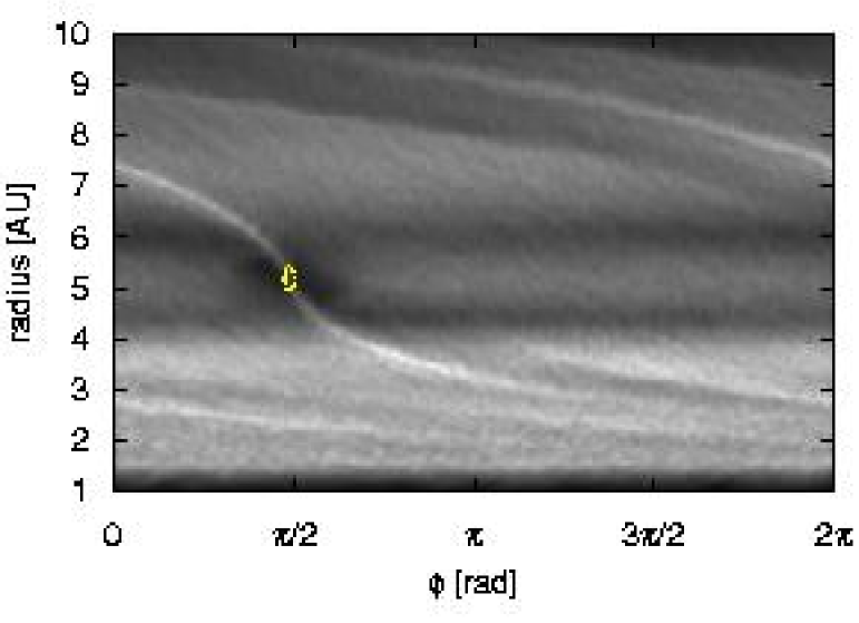
Figure 1: Greyscale plot of the surface density in the disc in the case of the reference model after 10 orbits of the protoplanet in the disc. The gap clearing has already started, and the spiral density wave pattern is visible throughout the disc. The circle represents the Roche lobe of the protoplanet according to Eggleton’s formula.

Figure 2: Evolution of the azimuthally averaged surface density for five different times in the case of the reference model. The planet has a fixed orbit at $5.2$ AU.

The radial size of the gap depends only slightly on the viscosity, as can be seen in Fig. 3, where the surface density is plotted for three simulation runs with different kinematic viscosity: $\nu=\nu_{0}=10^{15}$ $\mathrm{cm^{2}/s}$ (reference model), $\nu=2\nu_{0}$, and $\nu=4\nu_{0}$. A higher viscosity leads to a faster radial motion of the gas in the disc, and thus to more loss at the inner boundary, which results in a slightly lower density profile after the same number of orbits. A similar behaviour was found by Kley (1999). Because in Fig. 3 the simulation time is rather short compared with the viscous timescales, the gap structure looks very similar in each case. The differences may become more pronounced for longer simulation runs.

Figure 3: Influence of the kinematic viscosity parameter on the gap size. The azimuthally averaged surface density is plotted for three different viscosities in units of $\nu_{0}=10^{15}$ $\mathrm{cm^{2}/s}$ after 100 orbits of the protoplanet. The planet has a fixed orbit with a radial distance of $5.2$ AU.

Unlike the viscosity, the scale height has a severe impact on the depth of the gap as can be seen in Fig. 4. There, the surface density of the disc after 100 orbits of the protoplanet is plotted for the scale heights $H/r=0.1$, $H/r=0.05$, and $H/r=0.025$. The smaller the scale height, the lower the temperature and the deeper the gap, as can be seen clearly. Additionally, the spiral density wave pattern gets tighter as the sound speed is lower for smaller scale heights.

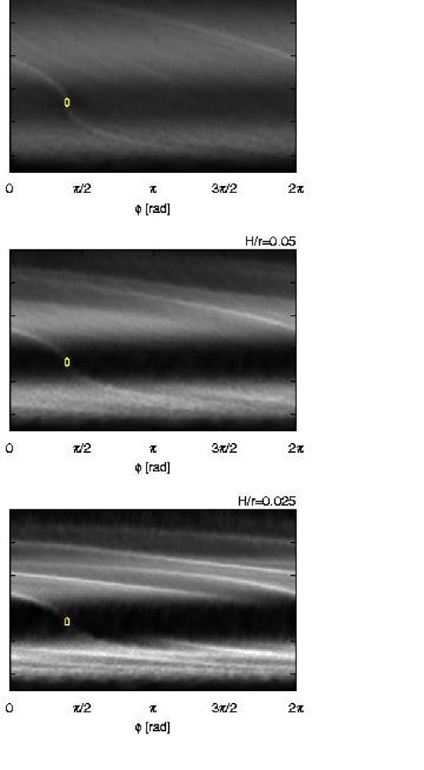
Figure 4: Influence of the scale height of the disc. The greyscale plot shows the surface density in the disc after 100 orbits of the protoplanet for three different scale heights.

4.1.2 Migration and accretion

In order to study the migration of the protoplanet we consider again the standard reference model of a jovian protoplanet in a circular orbit with radius $5.2$ $\mathrm{AU}$. To achieve a steady-state particle distribution we proceed as in the last section and let the system evolve until the gap is nearly fully developed before we allow the gravitational force of the particles to act on the protoplanet. Then the simulation is restarted and the trajectory of the planet is integrated as well. For the reference model we expect pure type II migration on a viscous timescale. For this simulation we used nearly 360 000 particles to model a disc with mass $3.33\times 10^{-3}$ M_☉ and $r_{\mathrm{in}}=1$ $\mathrm{AU}$, $r_{\mathrm{out}}=13\ \mathrm{AU}$. Particles that get closer to the protoplanet than 50 % of its Roche radius are taken out of the simulation and assumed to be accreted by the protoplanet. In one model, the mass of the accreted particles is added to the mass of the planet, in a second, the mass of the planet is fixed for all times. The total simulation time is about 30 000 years.

The evolution of the radial distances of the planets is shown in Fig. 5. Initially the migration rate is very high and about the same for both the planet with fixed mass and the planet with increasing mass. After 3 000 years the radial distances to the central object differ distinctly, with the more massive planet migrating slightly faster. Similar behaviour was found in numerical simulations by Nelson et al. (2000). The planet with a fixed mass ends up at an orbital distance of $4.5$ $\mathrm{AU}$ after 20 000 years, which would correspond to a steady-state migration rate of $3.5\times 10^{-5}\ \mathrm{AU/yr}$. The planet with increased mass has a radial distance of $4.27\ \mathrm{AU}$ after 30 900 years, or a steady-state migration rate of $1.4\times 10^{-4}\ \mathrm{AU/yr}$. As can be seen in Fig. 5, the migration rates are not constant but decrease considerably. This is caused primarily by the mass loss of the disc, leading to less gravitational interaction between the planet and the disc.

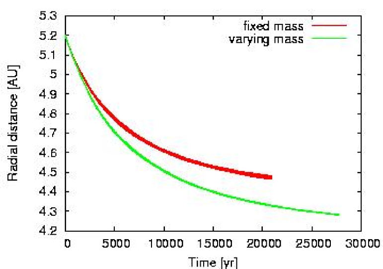
Figure 5: Evolution of the radial distance of the planet to the central object. The planet is initially located at a radial distance of $5.2$ $\mathrm{AU}$. In one model, the accreted mass is added to the planet’s mass, in the other the mass of the planet remains fixed.

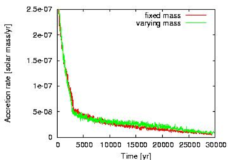
Figure 6: Evolution of the accretion rate on the planet for a planet with fixed mass and a planet with increasing mass. The planet is originally located at a radial distance of $5.2$ $\mathrm{AU}$, and migrates inwards as shown in Fig. 5.

The accretion rates of the planets for both models are presented in Fig. 6. The initial accretion rate of about $2.5\times 10^{-4}$ M${}_{\mathrm{jup}}/\mathrm{yr}$ drops rapidly in the first 3 000 years to a value of $5\times 10^{-5}$ M${}_{\mathrm{jup}}/\mathrm{yr}$ for both the planet with constant mass and the planet with increasing mass. At that time, the inner part of the accretion disc has vanished, as the material was either accreted by the protoplanet or by the central object. After the loss of the inner disc, the accretion rate decreases more slowly. Between 3 000 and 7 500 years of simulation time, the planet with increasing mass has a slightly lower accretion rate. The situation changes after 10 000 years, when the planet with the fixed mass accretes less. At the end of the simulation, both planets have about the same accretion rate of $10^{-5}$ M${}_{\mathrm{jup}}/\mathrm{yr}$, although the planet with mass accumulation has already doubled its mass. However, during that time the constant loss of material through the open boundaries and the accretion on the planet lead to a decrease in disc mass of nearly one magnitude, which has to be considered for comparisons to grid-based simulations with closed boundaries.

4.2 Two planets

As it is generally assumed that the mutual interaction of gravitating objects in an accretion disc can finally lead to eccentric orbits, we have included another protoplanet into our simulations.

4.2.1 Gap formation

For the simulation with two protoplanets the setup was changed as follows: one protoplanet is located at a distance of $5.2\ \mathrm{AU}$ from the central gravitating object, the other one at twice that. The kinematic viscosity parameter is again set to $10^{15}$ $\mathrm{cm^{2}/s}$, and the disc scale height is $0.05$. Now the outer radius of the disc is $20\ \mathrm{AU}$, and the inner boundary is set to $2\mathrm{AU}$. The number of particles in this run was $320\,000$ and the disc mass was set to $10^{-2}$ M_☉. The evolution of the density in the disc is shown in Fig. 7. As in the case of a single jovian planet, gap formation starts immediately after the beginning of the simulation. This happens for each planet individually, until the particles between the inner and outer planet have been accreted by the inner planet, and a common gap has formed. The innermost region of the disc has already vanished after 200 orbits of the inner planet.

Figure 7: Evolution of the azimuthally averaged surface density in the case of two protoplanets in the disc. The number of orbits of the inner planet is indicated. The inner planet is located at $5.2\ \mathrm{AU}$, the outer planet at twice that distance from the central object.

4.2.2 Migration and accretion

After 200 orbits of the inner planet, the simulation is restarted and the trajectories of the two planets are integrated to examine their migration. The evolution of the semi-major axis of the two planets is shown in Fig. 8 for the next 30 000 years. During the first 5 000 years the inner planet mainly stays on its orbital radius around the central star because it is not surrounded anymore by disc material (see Fig. 7) which could exert torques. On the other hand the outer planet migrates inwards due to the action of the outer disc, resulting in a radial approach of the two planets. As the orbital distance of the two planets decreases, they capture each other in a 2:1 mean motion resonance at approximately $t=7\,500$ years. Upon capture their eccentricities slowly increase, as can be seen in Fig. 9. By the end of the simulation, the eccentricity of the outer planet has grown to $0.1$ and the eccentricity of the inner planet to $0.18$. In the end, the planets have reached masses of $1.34$ (inner planet) and $2.9$ M_jup (outer planet), respectively. The mass of the disc changed from $10^{-2}$ M_☉ at the start of the simulation to $5.64\times 10^{-3}$ M_☉ at the end. After all, only 20 % of the mass lost by the disc have been accreted by the protoplanets. The resonant capture and overall evolution of this system is nearly identical to that described in Kley (2000).

Figure 8: Evolution of the semi-major axis of the two protoplanets. The initial parameters of the planets are the same as in Fig. 7, but now the trajectories of the planets are integrated

.

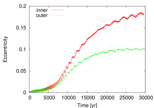
Figure 9: Evolution of the eccentricities of the two protoplanets during the migration, same simulation as presented in Fig. 8

.

5 Discussion

In the case of a single jovian planet we obtain the same influence of the disc scale height on the gap formation and on the structure of the spiral wave pattern as found already by several other authors (see, e.g., Bryden et al. 1999; Kley 1999), and as postulated by the theory. For the parameters of the reference model, Eq. (13) yields a migration rate of $4.13\times 10^{-5}\ \mathrm{AU/yr}$ for pure type II migration, for a planet located at a radial distance of $5.2\ \mathrm{AU}$. We find migration rates of the same order of magnitude by averaging over the complete simulation time. The migration rate for this simulation agrees well with migration rates found by D’Angelo et al. (2003), who examined the migration and growth of one protoplanet in a disc for various initial planet masses, using a grid-based method and closed boundary conditions.

Interestingly, the accretion rate for a planet with a fixed mass and a planet with increasing mass do not differ considerably at the end of a simulation time of 30 000 years. Presumably due to the loss of disc material at the open boundaries, the resolution is too coarse to resolve the difference correctly. After a simulation time of 15 000 years, the accretion rate onto the planets is about $2.5\times 10^{-5}\ \mathrm{M_{jup}/yr}$ for our reference model with a kinematic viscosity coefficient of $10^{15}\ \mathrm{cm^{2}/s}$. This value agrees well with the results from simulations performed by Lubow et al. (1999), who used the ZEUS hydrodynamics code to simulate disc accretion onto high-mass planets. They find an accretion rate of $2.13\times 10^{-5}\ \mathrm{M_{jup}/yr}$, which is half the value that was published by Kley (1999). However, Lubow et al. (1999) use different boundary conditions, namely reflecting closed boundaries at the inner edge of the disc, and open boundaries at the outer edge. The results of the simulations by Bryden et al. (1999) provide accretion rates in the same range, although they use an initial density profile which is constant throughout the disc. Extensive simulations with three different grid codes, nirvana, rh2d, and fargo, by Nelson et al. (2000) provide comparable accretion rates for a jovian planet.

For a single planet in the accretion disc the orbit remains circular, although the planet migrates towards the central star. This suggests that the gravitational interaction between the planet and the protoplanetary disc cannot excite a change in the eccentricity of the orbit of the planet, at least for low mass planets (Papaloizou et al. 2001). Therefore, in systems with a single extra-solar planet mostly circular orbits should be expected. This clearly appears to be in contradiction to the observations, and is why different mechanisms, e.g. resonances, for the evolution of high eccentricities in single-planet systems have to be assumed.

We have found that a number of $360\,000$ SPH-particles, which has been used in the simulation of migration and planet accretion, is sufficient in 2D to resolve an expected accretion rate of several $10^{-5}\ \mathrm{M_{jup}/yr}$. However, the use of an artificial bulk viscosity is essential, as extensive test calculations have shown. Without the use of this additional viscosity, the particle orbits penetrate each other, density shock waves cannot be resolved, and even the formation of the gap may be suppressed. Note that in contrast to the normally used artificial $\alpha$-viscosity approach (see Monaghan & Gingold (1983)) which leads to an effective physical shear viscosity (Nelson et al. 1998), this artificial bulk viscosity has very little impact on the shear kinematic viscosity in the disc, as can be seen in appendix A.

The number of SPH-particles was not high enough though to study the flow around the protoplanet within its Hill radius, as was done by D’Angelo et al. (2002) using nested-grid techniques. This would have made it possible to examine the accretion process onto the protoplanet more precisely. D’Angelo et al. (2002) find the formation of a so-called proto-jovian disc around the protoplanet which dominates the accretion process onto the planet. However, in our simulations the spatial resolution was too low to resolve the formation of such a disc.

Generally, SPH seems to be slightly more computationally expensive for this kind of application than comparable simulations with grid-based schemes. This is mostly due to the intrinsic noise of the particle method that requires a comparatively high particle number to achieve a similar spatial resolution. The advantage of this numerical method is its Lagrangian nature, which allows an easy treatment of open boundaries and complex geometries, like multiplanetary systems.

In order to study the evolution of a protoplanetary system with several planets, we included a second protoplanet in the simulation. After the first 200 orbits of the inner planet, the inner disc has already nearly vanished leading to a lower accretion and migration rate of the inner planet in comparison to the outer planet. Due to different migration speeds of the two planets they approach each other radially and are eventually captured into a 2:1 mean motion resonance. Upon capture, the dynamical interaction between the two planets increases and their eccentricities begin to grow considerably. This resonant behaviour has been found and investigated numerically already by several authors (e.g. Kley 2000; Nelson & Papaloizou 2002; Lee & Peale 2002; Kley et al. 2004). Depending on the subsequent evolution (distance of migration and damping), the system might become unstable eventually.

Thus, the gravitational interaction between protoplanets in the disc can explain the appearance of resonant extra-solar planets with high eccentricities as found for example in GJ 876, HD 82943, or 55 Cnc.

6 Conclusion

With the presented calculations we have modelled the dynamical evolution of a protoplanet embedded in a disc using the Lagrangian particle method SPH. The SPH-representation of the shear viscosity allows accurate treatment of the viscosity of the system, and the use of a newly introduced artificial bulk viscosity term in the Navier-Stokes equation inhibits mutual particle penetration. Our investigations comprised the evolution of a single Jovian-like protoplanet in a protoplanetary accretion disc, including the accretion of gas onto the planet and the migration of the planet through the disc. Moreover, we examined the effects on migration if two planets are located in the disc.

According to our simulations, gap formation does not inhibit accretion onto the protoplanet. Our simulations indicate that a protoplanet can grow up to several Jupiter masses before it has migrated to the central star. The simulations with two protoplanets show a possible mechanism for the formation of a two-planet system with a lower-mass planet near the central star and a more massive planet with a larger semi-major axis. The results of our SPH simulations compare favourably with those of grid codes. Although the computational costs are rather high, and therefore SPH seems to be less effective to model this problem, it is well suited to verify simulation results achieved with other, grid-based numerical schemes because of its completely different numerical approach. Moreover, it may be useful for 3D-simulations or self-gravitating flows.

Appendix A Numerical shear

To measure the intrinsic numerical shear viscosity of the new bulk viscosity approach, we have performed several test simulations of the viscously spreading ring, a model representing an idealised accretion disc orbiting a point mass. Because an analytic solution exists for this model (originally stated by Lüst (1952) and later by Lynden-Bell & Pringle (1974)), it is frequently used as a test problem for numerical codes developed to simulate accretion discs (e.g., Speith & Riffert (1999); Kley (1999)).

Usually, modelling the physical shear viscosity by implementing the viscous stress tensor according to Eq. (16) is sufficient to simulate the evolution of the viscous ring. This can be seen in Fig. 10 where the results of an SPH simulation with only physical viscosity, i.e. without any artificial viscosity, is shown. Plotted is the azimuthally averaged surface density over radius (the radial coordinate is normalized to the radius of the initial peak, $R_{0}$, and the surface density is normalized to the total mass of the accretion ring, $M/R_{0}^{2}$). For the kinematic viscosity we chose $\nu=\nu_{0}=10^{15}$ $\mathrm{cm^{2}/s}$, the value also used in the simulations of the protoplanetary disc. The solid line represents the averaged SPH results after a simulation of $3\times 10^{5}$ sec, the dashed-dotted line the results after $6\times 10^{5}$ sec, while the dashed line indicate the initial distribution, and the dotted lines denote the analytic solutions, respectively. The overall time evolution of the ring is reproduced very well. The appearing oscillations and deviations from the analytic solutions are mainly caused by a secular viscous instability inherent to the ring model (Speith & Kley 2003).

Figure 10: Evolution of the azimuthally averaged surface density of the viscous ring at three different times, using only physical viscosity in the simulation. Dotted lines denote the analytic solutions.

However, applying only physical viscosity according to Eq. (16) is insufficient to simulate the dynamical evolution of a protoplanet in a disc, because interpenetration of SPH particles occurs such that the spiral density wave pattern in the disc cannot be resolved. This problem is reliably prevented by the new artificial bulk viscosity presented in Eq. (19) in combination with the XSPH-scheme of Eq. (22). To test for any spurious numerical shear viscosity that may be introduced by the usage of these algorithms, a simulation similar to that presented in Fig. 10 was performed with additional artificial bulk viscosity, where we set $f=0.5$ and XSPH is switched on with $x=0.5$. The results are shown in Fig. 11, where the quantities equivalent to those in Fig. 10 are plotted. As can be seen, the global evolution of the viscous ring, which is very sensitive to the effective shear viscosity in the simulation, seems not to be affected at all by the new artificial viscosity approach.

Figure 11: Evolution of the azimuthally averaged surface density of the viscous ring at three different times, additionally using artificial bulk viscosity and XSPH together with the physical viscosity. Dotted lines denote the analytic solutions.

This can be tested further by a simulation where only artificial bulk viscosity is used. The results are shown in Fig. 12. Any evolution of the viscous ring away from the initial distribution, which is indicated by the dashed line, has to be due to inherent numerical shear in the simulation. It can clearly be seen that the intrinsic effective shear of the artificial bulk viscosity approach is very small. A more quantitative analysis gives a value of less than 9 % of $\nu_{0}$, which can be neglected in all our simulations of the protoplanetary disc. Note that the numerical effective shear viscosity is not constant throughout the ring but seems to be higher at the edges, especially at the inner edge, than in the centre.

Figure 12: Evolution of the azimuthally averaged surface density of the viscous ring at three different times, applying only artificial bulk viscosity. The dotted line represents the initial analytic solution.

It has turned out that it is necessary to use the XSPH-algorithm in addition to the artificial bulk viscosity to prevent mutual particle penetration more effectively. This can be seen in Fig. 13, where two different simulations of the reference model of the protoplanetary disc are shown, in the upper panel with XSPH switched on and in the lower panel with XSPH switched off. The surface density is plotted in greyscale, similar to the result presented in Fig. 1, but only for the inner part of the disc and in Cartesian coordinates. Both plots show basically the same features, but in the case with XSPH the structures are more distinct and better resolved, while in the case without XSPH the distribution is more diffuse.

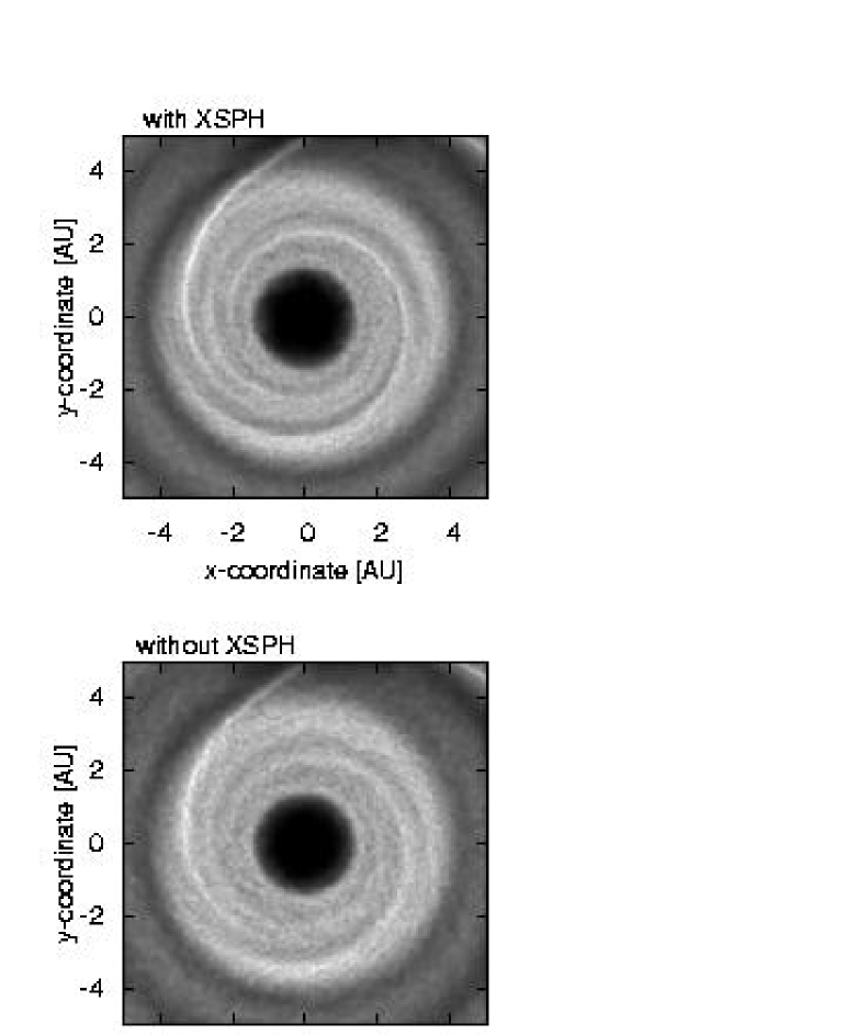
Figure 13: Greyscale plots of the surface density of the inner part of the protoplanetary disc in the case of the reference model similar to Fig. 1 but in Cartesian coordinates, with (upper panel) and without (lower panel) using the XSPH-algorithm. Note that the planet cannot be seen on these plots, since it is located at a radial distance of $5.2\leavevmode\nobreak\ \mathrm{AU}$.

For the sake of completeness it should be mentioned, that a frequently used very efficient different approach to prevent particle interpenetration is the usual artificial viscosity introduced by Monaghan & Gingold (1983), and there especially the quadratic $\beta$-term. However, this artificial viscosity suffers from a high level of spurious intrinsic shear. This becomes obvious in the simulation of the viscous ring shown in Fig. 14, where only this artificial viscosity is used with a rather small value of $\beta=1$. The effective physical shear is already of the order of $\nu_{0}$.

Figure 14: Evolution of the azimuthally averaged surface density of the viscous ring at three different times, applying only the usual artificial viscosity. The dotted line represents the initial analytic solution.

References

- Artymowicz & Lubow (1996) Artymowicz, P. & Lubow, S. H. 1996, ApJ, 467, L77
- Beckwith et al. (2000) Beckwith, S. V. W., Henning, T., & Nakagawa, Y. 2000, Protostars and Planets IV, 533
- Beckwith & Sargent (1996) Beckwith, S. V. W. & Sargent, A. I. 1996, Nature, 383, 139
- Benz (1990) Benz, W. 1990, in Numerical Modelling of Nonlinear Stellar Pulsations Problems and Prospects, 269
- Boss (2001) Boss, A. P. 2001, ApJ, 563, 367
- Boss (2003) Boss, A. P. 2003, in Lunar and Planetary Institute Conference Abstracts, 1075
- Bryden et al. (1999) Bryden, G., Chen, X., Lin, D., Nelson, R. P., & Papaloizou, J. C. 1999, ApJ, 514, 344
- Bryden et al. (2000) Bryden, G., Lin, D. N. C., & Ida, S. 2000, ApJ, 544, 481
- Bubeck et al. (1999) Bubeck, T., Hipp, M., Hüttemann, S., et al. 1999, Parallel SPH on Cray T3E and NEC SX-4 using DTS, ed. E. Krause & W. Jäger (Berlin, Heidelberg, New York: Springer)
- D’Angelo et al. (2002) D’Angelo, G., Henning, T., & Kley, W. 2002, A&A, 385, 647
- D’Angelo et al. (2003) D’Angelo, G., Kley, W., & Henning, T. 2003, ApJ, 586, 540
- Eggleton (1983) Eggleton, P. P. 1983, ApJ, 268, 368
- Flebbe et al. (1994) Flebbe, O., Muenzel, S., Herold, H., Riffert, H., & Ruder, H. 1994, ApJ, 431, 754
- Gingold & Monaghan (1977) Gingold, R. A. & Monaghan, J. J. 1977, MNRAS, 181, 375
- Goldreich & Tremaine (1979) Goldreich, P. & Tremaine, S. 1979, ApJ, 233, 857
- Goldreich & Tremaine (1980) —. 1980, ApJ, 241, 425
- Ivanov et al. (1999) Ivanov, P. B., Papaloizou, J. C. B., & Polnarev, A. G. 1999, MNRAS, 307, 79
- Kallenbach et al. (2000) Kallenbach, R., Benz, W., & Lugmair, G. W. 2000, in From Dust to Terrestrial Planets, 1
- Kley (1999) Kley, W. 1999, MNRAS, 303, 696
- Kley (2000) —. 2000, MNRAS, 313, L47
- Kley et al. (2003) Kley, W., Peitz, J., & Bryden, G. 2003, astro-ph/0310321, A&A, in press
- Korycansky & Papaloizou (1996) Korycansky, D. G. & Papaloizou, J. C. B. 1996, ApJS, 105, 181
- Lee & Peale (2002) Lee, M. H. & Peale, S. J. 2002, ApJ, 567, 596
- Lin & Papaloizou (1985) Lin, D. N. C. & Papaloizou, J. 1985, in Protostars and Planets II, 981–1072
- Lin & Papaloizou (1993) Lin, D. N. C. & Papaloizou, J. C. B. 1993, in Protostars and Planets III, 749–835
- Lin et al. (2000) Lin, D. N. C., Papaloizou, J. C. B., Terquem, C., Bryden, G., & Ida, S. 2000, Protostars and Planets IV, 1111
- Lubow et al. (1999) Lubow, S., Seibert, M., & Artymowicz, P. 1999, ApJ, 526, 1001
- Lucy (1977) Lucy, L. B. 1977, AJ, 82, 1013
- Lufkin et al. (2003) Lufkin, G., Quinn, T., Wadsley, J., Stadel, J., & Governato, F. 2003, ArXiv Astrophysics e-prints, 5546
- Lüst (1952) Lüst, R. 1952, Z. Naturforschg., 7a, 87
- Lynden-Bell & Pringle (1974) Lynden-Bell, D. & Pringle, J. E. 1974, MNRAS, 168, 603
- Marcy et al. (2000) Marcy, G. W., Cochran, W. D., & Mayor, M. 2000, Protostars and Planets IV, 1285
- Mayer et al. (2002) Mayer, L., Quinn, T., Wadsley, J., & Stadel, J. 2002, Science, 298, 1756
- Mayor & Queloz (1995) Mayor, M. & Queloz, D. 1995, Nature, 378, 355
- Monaghan (1989) Monaghan, J. J. 1989, Journal of Computational Physics, 82, 1
- Monaghan (1992) Monaghan, J. J. 1992, Annual Review Astronomy Astrophysics, 30, 543
- Monaghan & Gingold (1983) Monaghan, J. J. & Gingold, R. A. 1983, Journal of Computational Physics, 52, 374
- Nelson et al. (1998) Nelson, A. F., Benz, W., Adams, F. C., & Arnett, D. 1998, ApJ, 502, 342
- Nelson & Papaloizou (2002) Nelson, R. P. & Papaloizou, J. C. B. 2002, MNRAS, 333, L26
- Nelson et al. (2000) Nelson, R. P., Papaloizou, J. C. B., Masset, F., & Kley, W. 2000, MNRAS, 318, 18
- Ohtsuki et al. (2002) Ohtsuki, K., Stewart, G. R., & Ida, S. 2002, Icarus, Volume 155, Issue 2, pp. 436-453 (2002)., 155, 436
- Papaloizou & Lin (1984) Papaloizou, J. & Lin, D. N. C. 1984, ApJ, 285, 818
- Papaloizou et al. (2001) Papaloizou, J. C. B., Nelson, R. P., & Masset, F. 2001, A&A, 366, 263
- Papaloizou et al. (1999) Papaloizou, J. C. B., Terquem, C., & Nelson, R. P. 1999, in Astrophysical Discs – an EC summer school, Conference Series, ed. J. A. Sellwood & J. Goodman, Vol. 160 (Astronomical Society of the Pacific), 186
- Perryman (2000) Perryman, M. A. C. 2000, Reports of Progress in Physics, 63, 1209
- Pollack et al. (1996) Pollack, J. B., Hubickyj, O., Bodenheimer, P., et al. 1996, Icarus, 124, 62
- Sekiya et al. (1987) Sekiya, M., Miyama, S. M., & Hayashi, C. 1987, Earth Moon and Planets, 39, 1
- Shakura & Sunyaev (1973) Shakura, N. & Sunyaev, R. 1973, A&A, 24, 337
- Speith & Kley (2003) Speith, R. & Kley, W. 2003, A&A, 339, 395
- Speith & Riffert (1999) Speith, R. & Riffert, H. 1999, JCAM, 109, 231
- Syer & Clarke (1995) Syer, D. & Clarke, C. J. 1995, MNRAS, 277, 758
- Terquem et al. (2000) Terquem, C., Papaloizou, J. C. B., & Nelson, R. P. 2000, in From Dust to terrestrial planets, ed. W. Benz, R. Kallenbach, G. Lugmair, & F. Podosek
- Ward (1997) Ward, W. R. 1997, Icarus, 126, 261
- Lufkin et al. (2004) Lufkin, G., Quinn, T., Wadsley, J., Stadel, J., & Governato, F. 2004, MNRAS, 347, 421
- Kley et al. (2004) Kley, W., Peitz, J., & Bryden, G. 2004, A&A, 414, 735