Isochrone ages for field dwarfs: method and application to the age-metallicity relation

Abstract

A new method is presented to compute age estimates from theoretical isochrones using temperature, luminosity and metallicity data for individual stars. Based on Bayesian probability theory, this method avoids the systematic biases affecting simpler strategies, and provides reliable estimates of the age probability distribution function for late-type dwarfs. Basic assumptions about the a priori parameter distribution suitable for the solar neighbourhood are combined with the likelihood assigned to the observed data to yield the complete posterior age probability. This method is especially relevant for G dwarfs in the 3-15 Gyr range of ages, crucial to the study of the chemical and dynamical history of the Galaxy. In many cases, it yields markedly different results from the traditional approach of reading the derived age from the isochrone nearest to the data point. We show that the strongest effect affecting the traditional approach is that of strongly favoring computed ages near the end-of-main-sequence lifetime. The Bayesian method compensates for this potential bias and generally assigns much higher probabilities to lower, main-sequence ages, compared to short-lived evolved stages. This has a strong influence on any application to galactic studies, especially given the present uncertainties on the absolute temperature scale of the stellar evolution models. In particular, the known mismatch between the model predictions and the observations for moderately metal-poor dwarfs ($-1<[Fe/H]<-0.3$) has a dramatic effect on the traditional age determination.

We apply our method to the classic sample of Edvardsson et al. (1993), who derived the age-metallicity relation (AMR) of a sample of 189 field dwarfs with precisely determined abundances. We show how most of the observed scatter in the AMR is caused by the interplay between the systematic biases affecting the traditional age determination, the colour mismatch with the evolution models, and the presence of undetected binaries. Using new parallax, temperature and metallicity data, our age determination for the Edvardsson et al. sample indicates that the intrinsic dispersion in the AMR is at most 0.15 dex and probably lower. In particular, we show that old, metal-rich objects ($[Fe/H]\sim 0.0$ dex, $age>5$ Gyr) and young, metal-poor objects ($[Fe/H]<-0.5$ dex, $age<6$ Gyr) in many observed AMR plots are artifacts caused by a too simple treatment of the age determination, and that the Galactic AMR is monotonically increasing and rather well-defined. Incidentally, our results tend to restore confidence in the method of age determination from chromospheric activity for field dwarfs.

1 Introduction

Isochrone ages for field dwarfs – Bayesian approach

Theoretical stellar evolution models have proved spectacularly successful at explaining the position of stars in the colour-magnitude diagram (CMD), as a function of only three parameters: mass, age and metallicity. Comparison of the mean sequences of open and globular clusters with theoretical isochrones forms the basis of age estimations in astrophysics. Although second-order discrepancies subsist such as the subdwarf locus, the slope of the red giant branch, the width of the main sequence or the distance of the Pleiades, the method has now been improved to the degree of reaching a relative accuracy better than 10 percent for cluster ages from theoretical isochrones (see e.g. Rosenberg et al. 2002 for globular clusters).

In principle, this method can also be applied to individual stars. The model predictions can be interpolated to associate a given star’s observed parameters, by inverting the relation given by the models between the physical parameters (mass, temperature, abundances) and observable parameters such as luminosity, temperature, metallicity, colour and magnitude. In particular, because late-F and G dwarfs have lifetimes comparable to the age of the Galaxy, deriving individual ages for field F and G dwarfs in the solar neighbourhood is of crucial importance to study the chemical and dynamical history of the Galactic disc. In practice, however, deriving ages for late-type dwarfs turns out to be difficult. For the ages typical of galactic populations, from $\sim$ 1 Gyr up to the maximum age of stars in the Galaxy, the model isochrones are separated only by small distances in observable parameter space on and near the main sequence, and high accuracy on the temperature, distance and metallicity determinations, as well as high confidence in the absolute temperature and metallicity scales of the models and observations, are needed to obtain meaningful results for individual ages.

One landmark study in that field is Edvardsson et al. (1993, hereafter E93), who obtained very accurate multi-element abundances for 189 field F and G stars and computed ages spanning the whole lifetime of the Galactic disc. They derived the ages for individual stars in their sample by comparison with Vandenberg (1985) isochrones. Their results have subsequently been recomputed with more recent Bertelli et al. (1994) isochrones by Ng & Bertelli (1998). Chen et al. (2000) have added multi-element metallicity data for 90 more disc stars, and Bensby, Felzing & Lundström (2003) for 66 stars.

Following the availability of Hipparcos parallaxes for most nearby F and G dwarfs, ages have been derived for much larger sets of data (e.g. Asiain et al. 1999; Feltzing et al. 2001; Ibukiyama & Arimoto 2002). The publication of the large Geneva-Copenhagen solar-neighbourhood survey (Nordström et al. 1999, hereafter GCS), with metallicities, distances and Strömgren photometry for more than 16’000 local F and G dwarfs, is likely to prompt more such studies in the near future.

Another important method to derive ages for field F-G dwarfs is the use of chromospheric activity as an age indicator (e.g. Kraft 1967, Noyes et al. 1984). It has been applied to a large sample of disc F and G dwarfs by Rocha-Pinto et al. (2000). The results of the isochrone and chromospheric age estimates are not showing satisfactory agreement.

Deriving age estimates from isochrones for individual stars is an inverse problem. The tracks calculated from theoretical evolution models define a function $\mbox{\boldmath$Y$}={\cal F}(\mbox{\boldmath$X$})$ relating the input physical parameters $X$ (age, mass, abundance) to the observable parameters $Y$ (e.g. temperature, luminosity, metallicity). The objective is to derive estimates of the physical parameters $X$ from the observed $Y$.

All studies quoted above have estimated isochrone ages for individual stars by selecting the isochrone nearest to the object in data space, i.e. computing ${\cal F}^{-1}(\mbox{\boldmath$Y$})$. The uncertainties affecting the resulting ages are estimated by probing the ${\cal F}^{-1}$ around ${\cal F}^{-1}(\mbox{\boldmath$Y$})$ according to the uncertainties affecting $Y$.

However, in practice, there are two conditions for the inverse function ${\cal F}^{-1}$ to provide an unbiased estimator of the real $X$:

1. the function must be reasonably linear within the uncertainties on $Y$.
   

2. the uncertainties on $Y$ must be much smaller than the variations in its a priori probability distribution.

These two conditions are generally satisfied for the age determination of early-type stars at the bright end of the main sequence, with ages in the range 0-3 Gyr. In this regime, the observational uncertainties are generally smaller than the range over which the isochrones curve, and over which the a priori density varies. It is much less clear that the conditions are respected for later-type dwarfs, with ages in the 3-15 Gyr range. In this range, condition (1) is not satisfied, because the isochrones are densely packed and highly curved within the observational uncertainties. Condition (2) is not satisfied either: under any reasonable assumption, the a priori distribution of the observables can vary enormously within the uncertainties on $Y$. For instance, varying the luminosity within one or two sigma can move an observation from the main-sequence into the Hertzsprung gap, where the a priori density is an order of magnitude lower, or even below the ZAMS, where the a priori density is zero. Therefore, the isochrone age from the simple inversion of the function defined by the evolution models can suffer from significant systematic biases. Because those objects are the most interesting to study the history and evolution of the Galaxy (age range 3-15 Gyr), it is important to derive realistic and unbiased age estimates for them.

When condition (1) is not satisfied, one way to obtain an unbiased estimator is to consider the complete probability distribution function (’pdf’) of $Y$ given its uncertainties, $\mbox{prob}(\mbox{\boldmath$Y$})$, and to compute the corresponding distribution of $\mbox{prob}\left({\cal F}^{-1}(\mbox{\boldmath$Y$})\right)$. The resulting probability distribution function is known as the likelihood. Methods based on the likelihood can provide reliable estimators when the function relating the observed values to the unknown parameters is highly non-linear.

When condition (2) is not satisfied, even estimators based on the likelihood will be biased. One common way to deal with the problem is to build simulations of the whole procedure, estimate the systematic biases from the simulations, and then correct the results with a posteriori compensations for the biases. However, Bayesian probability theory offers a much more robust method to obtain unbiased estimates in that case. The Bayesian approach includes both the likelihood and the a priori distribution of the parameters to compute the complete, unbiased posterior probability distribution.

When possible, fully Bayesian analyses are often avoided because of their large demand in computing time and their conceptual difficulty. In recent years however, their use has become more and more frequent, following both the increase in computing power and the development of the theory. For a general introduction to Bayesian data analysis see Sivia (1996), for a very clear and detailed presentation see Jaynes (2003), and for a rapid overview centered on astrophysical applications see Loredo (1990). In this paper, we assume that the notations and concepts of probability theory are familiar to the reader. We are mostly using notations as in Sivia (1996). Cases that necessitate a Bayesian analysis are rare. In general, measurement uncertainties are much smaller than the range of the a priori distribution. Bayesian analyses are necessary in the case of high relative errors on single-case estimates. They have been used to derive the most likely value of the cosmological parameters (e.g. Slosar et al. 2003) and to analyse the neutrino data of SN1987A (Loredo 1990). Another example is the case of the study of the bias affecting trigonometric parallaxes (Lutz & Kelker 1973): In the wake of the Hipparcos astrometric satellite mission, an extensive literature has appeared on the subject (Oudmaijer, Groenewegen & Schrijver 1998; Pont 1999; Reid 1999; Arenou & Luri 2002; Smith 2003). In that case, it was found that with high-relative-error parallax measurements ($\sigma_{\varpi}/\varpi>\sim 0.2$), straightforward statistical methods brake down, and the effect of the prior begins to become so dominant that hardly anything meaningful can be derived about the value of the distance independently of the a priori assumptions. It is now accepted that a limit of $\sim$10 percent has to be put on $\sigma_{\varpi}/\varpi$ to derive robust distance estimates from trigonometric parallaxes independently of further assumptions. The Lutz-Kelker effect is a typical Bayesian effect showing when the shape of the prior has to be taken into account.

In this paper, which is intended both as a reconsideration of previous data and as a preparation for the coming analysis of new large samples, we point out fundamental features in the analysis of ages for individual stars that have been overlooked by all previous studies that we are aware of, and that can profoundly affect the results. We examine in what way the age determination can be improved using probability theory. We propose a method to compute the Bayesian age probability distribution for field stars and compare them to likelihood estimates (Part One). We then focus on the E93 sample as an illustrative application (Part Two).

The E93 study and the Galactic age-metallicity relation

The E93 sample of 189 stars in the solar neighbourhood still provides one of the most accurate and extensive bases for the study of the chemical evolution of the Galactic disc. In particular, many authors subsequently accepted their age-metallicity plot (repeated in Fig. 9a, but see companion figures) and their interpretation of a very substantial spread of $[\textrm{Fe/H}]$ for a given age in the solar neighbourhood. The plot shows a large intrinsic scatter at ages between 3 and 10 Gyr, with a standard dispersion of $\simeq 0.24$ dex and almost no age-metallicity relation in this range. The age-metallicity plot for their sample is often presented as ”the age-metallicity relation of the Galaxy” and a dispersion of the order of 0.25 dex – corresponding to a total range of $\sim$ 0.6 to 0.8 dex – in metallicity at a given age has been taken as an observational requirement that the models of the Galaxy are requested to meet (e.g. Carraro et al. 1998). However, more recently, Garnett & Kobulnicky (2000) have revealed an important dependence of the metallicity dispersion with distance in the E93 sample, indicating that the age metallicity relation (AMR) from E93 may have been affected by strong systematic biases.

Rocha-Pinto et al. (2000) have studied the dispersion of the AMR with age determinations based on chromospheric activity. Their ages are only weakly correlated with the isochrone ages, and they find a low intrinsic dispersion of the AMR. This result is particularly significant given the statistical implausibility of decreasing the dispersion of the AMR with added uncertainties.

The age-metallicity relation is one of the most important observational constraints on models of the evolution of the Galaxy. It expresses how stellar formation has enriched the interstellar medium over time, and therefore depends on the star formation rate, the chemical yields, the efficiency of recycling, infall and outflow, and the amount of mixing in the gas. Because the shear induced by differential galactic rotation spreads stars and gas around all galactic azimuths in a few rotations, theoretical models commonly assume a metallicity depending only on time and galactocentric radius (e.g. Chiappini et al. 1997). Several observations support this assumption. The inhomogeneities in the abundance of the interstellar medium are small (Kobulnicky & Skillman 1996; Meyer, Jura & Cardelli 1998). $R\sim R_{0}$ Cepheids show a low abundance dispersion (Andrievsky et al. 2002); young open clusters show an abundance dispersion lower than 0.20 dex (Twarog 1980; Carraro et al. 1998). The indication from older open clusters is more ambiguous (Twarog 1980; Piatti et al. 1995; Carraro et al. 1998; Friel et al. 2002), showing a large scatter that can be mostly attributed to a radial metallicity gradient. Kotoneva et al. 2002a find that only a modest intrinsic scatter in the AMR is needed to fit the solar neighbourhood K-dwarfs data. In external spiral galaxies, the abundance dispersion of young features at a given galactocentric distance is typically much smaller than 0.2 dex (e.g. Kennicutt & Garnett 1996 for HII regions in M101).

In this context, the E93 result comes as a surprise, and a very difficult requirement to be met by the models. E93 computed the present Galactic orbits of their objects, and concluded that only a small part of the observed metallicity dispersion was due to orbital diffusion i.e. the fact that metal-richer and metal-poorer stars born at lower or higher galactocentric radii cross the solar neighbourhood. The remaining dispersion, covering a total range of the order of 0.6-0.8 dex at a given age, was taken to be the indication of a very high dispersion of the metallicity of the gas at a given time and galactocentric radius (or even a complete lack of correlation between age and metallicity, e.g. Feltzing et al. 2001). Such a result implies a very inefficient azimuthal mixing of the gas in the disc, or extremely frequent infall episodes, with pockets of gas of very different metallicities sharing a similar radius at a given time.

An alternative explanation for a high intrinsic dispersion was explored by Selwood & Binney (2002) and Lépine et al. (2003), who showed that radial migration of the stellar orbits without conservation of the angular momentum, for instance under the influence of spiral arm perturbations, could move stars in galactocentric radius by several kiloparsecs within the Galactic disc. This could bring together stars of the same age on similar orbits but formed at very different galactocentric radii, therefore with very different metallicities because of the radial metallicity gradient in the disc of the Galaxy.

In the second part of this article, we apply our age determination to the E93 sample as an illustration of our approach to the age determination, and conclude that – as correctly anticipated by Garnett & Kobulnicky (2000) – most of the ”cosmic” dispersion in the AMR of E93 is due to uncertainties in the ages, and that the data actually indicate a cosmic dispersion of less than 0.15 dex.

PART ONE: Age estimates from isochrones for individual late-type stars

2 Theoretical basis

2.1 Confrontation of the standard and Bayesian approach

The standard approach

Stellar evolution models define a function relating physical parameters to observable quantities:

$$\mbox{\boldmath$Y$}={\cal F}(\mbox{\boldmath$X$})$$

where $X$ are the physical input parameters, namely mass, age and abundance: $\mbox{\boldmath$X$}\equiv(m,t,z)$, and $Y$ are the observed quantities – observed or inferred directly from observations – e.g. temperature, luminosity and metallicity: $\mbox{\boldmath$Y$}\equiv(T,L,[\textrm{Fe/H}])$.

The standard approach to computing the age of an individual star from theoretical isochrones is to interpolate the stellar evolution tracks to find which age and mass value correspond to the same point as the star in the $(T,L,[\textrm{Fe/H}])$ space.

Interpolation between the models is needed to yield a value of ${\cal F}$ for all $(m,t,z)$ triplets. Given the observed values $T_{\mbox{\scriptsize obs}}$, $L_{\mbox{\scriptsize obs}}$ and $[\textrm{Fe/H}]_{\mbox{\scriptsize obs}}$, the standard approach thus inverts the relation ${\cal F}$ to find

$$(m_{o},t_{o},z_{o})={\cal F}^{-1}(T_{\mbox{\scriptsize obs}},L_{\mbox{\scriptsize obs}},[\textrm{Fe/H}]_{\mbox{\scriptsize obs}})$$

where the ”o” subscript denote the values for the considered object.

The function ${\cal F}$ is not strictly bijective because isochrones do sometimes cross each other in the $Y$ space. ${\cal F}^{-1}$ can be uniquely defined nevertheless by considering, when it is multiply defined, only the stage that is more slowly evolving. ${\cal F}^{-1}$, of course, is also undefined in the large portion of the $Y$ space that do not contain any evolution tracks.

A simple way to estimate the uncertainties on the $t_{o}$ age obtained by the inversion of the ${\cal F}$ function is to calculate the value on ${\cal F}^{-1}$ found by moving the data point according to the observational errors:

$$(m_{\pm\sigma},t_{\pm\sigma},z_{\pm\sigma})={\cal F}^{-1}(T_{\mbox{\scriptsize obs}}\pm\sigma_{\tiny T},L_{\mbox{\scriptsize obs}}\pm\sigma_{\tiny L},[\textrm{Fe/H}]_{\mbox{\scriptsize obs}}\pm\sigma_{\tiny[Fe/H]})$$

either one at a time or all at the same time.

A slightly more sophisticated approach is to compute ${\cal F}^{-1}$ over the whole $(\log T,L,[\textrm{Fe/H}])$ space, and to assign to each point the probability given by the distribution function of the observational uncertainties. For instance, if the observational uncertainties are described by Gaussian functions with dispersions $\sigma_{\tiny[Fe/H]}$, $\sigma_{\tiny\log T}$ and $\sigma_{\tiny\log L}$, then the recovered age distribution function is based on the likelihood function:

$${\cal L}(T,L,[\textrm{Fe/H}])=\ \frac{1}{\sigma_{\tiny[Fe/H]}\,\sigma_{\tiny T}\,\sigma_{\tiny L}\,(2\pi)^{3/2}}$$

$$\times\exp\frac{-(\log T_{\mbox{\scriptsize obs}}-\log T)^{2}}{2\sigma^{2}_{\tiny\log T}}\exp\frac{-(\log L_{\mbox{\scriptsize obs}}-\log L)^{2}}{2\sigma^{2}_{\tiny\log L}}$$

$$\times\exp\frac{-([\textrm{Fe/H}]_{\mbox{\scriptsize obs}}-[\textrm{Fe/H}])^{2}}{2\sigma^{2}_{[Fe/H]}}\$$ (1)

This likelihood is the conditional probability of a point being observed at $(T_{obs},L_{obs},[\textrm{Fe/H}]_{obs})$ given a true value of $(T,L,[\textrm{Fe/H}])$, or ${\cal L}(\textrm{observed,true})\equiv\mbox{prob}(\textrm{observed}|\textrm{true})$ where the ”$\mid$” symbol denotes conditional probabilities. The terms on the right result from the Gaussian distribution of the uncertainties. Instead of simply inverting the ${\cal F}$ function at the value of the data point, an age pdf can be obtained from the histogram in age of the likelihood over all possible ages:

$${\cal L}_{t}(t)=\int_{R}{\cal L}(T,L,[\textrm{Fe/H}])\,\mbox{d}[\textrm{Fe/H}]\,\mbox{d}T\,\mbox{d}L$$

where $R$ is the region in ($T,L,[\textrm{Fe/H}]$) space where the ${\cal F}^{-1}(T,L,[\textrm{Fe/H}])=t$. The maximum of ${\cal L}_{t}$ can be used as an estimator (maximum likelihood method).

Bayes’ theorem

However, $\mbox{prob}(\textrm{observed}\mid\textrm{true})$ is not really the probability that one is trying to determine when performing a measurement. One is not attempting to estimate the probability of the observed value assuming the true value, but indeed the value of the true quantity, given the observation, i.e. $\mbox{prob}(\textrm{true}|\textrm{observed})$.

These two quantities are related through Bayes’ theorem:

$$\mbox{prob}(H|D)=\frac{\mbox{prob}(D|H)}{\mbox{prob}(D)}\,\mbox{prob}(H)$$ (2)

where $H$ can be any set of hypotheses (in our case the true age value) and $D$ the observed data. The term on the left is called the posterior probability (the probability of $H$ given $D$, which is what one wants to determine), the numerator on the right is the likelihood (the probability distribution of $D$ assuming $H$, or the ”likelihood” of observing $D$ if $H$ is true). $\mbox{prob}(H)$ is the prior probability (what was known about $H$ a priori), and $\mbox{prob}(D)$ is a normalizing factor independent of $H$ (that can be ignored for our purposes). Therefore, according to Bayes’ theorem, the condition for the likelihood to be a good estimator of the posterior pdf is that the prior pdf can be neglected. Then Bayes’ theorem becomes $\mbox{prob}(H|D)\sim\mbox{prob}(D|H)={\cal L}(D,H)$.

The basic criterion to determine whether the prior probability distribution can be neglected in a given problem is to compare the scale of variation of the prior pdf with the scale of the observational uncertainties. If the uncertainties are much smaller than the scale over which the prior varies, then the likelihood ”overwhelms” the prior. This is the case for instance when the magnitude of a star is measured with an accuracy of, say, 0.01 mag. The prior pdf can vary from case to case, but a natural prior is to assume nothing on the magnitude, allowing for the star to be located at random in a 3-D space, which implies for the prior a dependence in $10^{0.6\cdot\Delta m_{v}}$, a variation of a factor $\sim$1.4 percent for each 0.01 magnitude. Thus the variation of the prior is negligible compared to the variation of the likelihood ($\sim$ 30 percent on $\sigma=0.01$ mag for a Gaussian distribution).

In some cases though, the prior pdf cannot be neglected. The prior probability varies a lot over the span of the observational uncertainties. In other words, previous knowledge indicates that one part of the likelihood distribution is much less probable than the other. For example, imagine measuring with very low accuracy the magnitude of a star picked up at random from the HD catalogue, and obtaining $m_{V}=7.0\pm 1.0$ mag. The likelihood is a Gaussian, $N(7,1)$. It would not result however that $6.0$ and $8.0$ are equally likely for the star’s actual magnitude, given the fact that faint stars are more numerous than bright stars by a factor $10^{0.6\cdot\Delta m_{v}}$ in a magnitude-limited survey (that is the prior $\mbox{prob}(H)$). After the measurement, $m_{V}>7$ is a much better estimate of the true magnitude, $\mbox{prob}(H|D)$, than $m_{V}<7$. At the other extreme, values $m_{V}\sim 9$ are much less likely than indicated by the function $N(7,1)$, because the HD catalogue has a magnitude limit $m_{V}\sim 8.5$. In this example the likelihood was not peaked enough to ”overwhelm” the prior, and the posterior pdf obtained through Bayes’ theorem resembles the prior more than the likelihood.

Another, more astrophysically relevant, such situation is the case of trigonometric parallaxes with high relative errors (see Introduction for references). The prior distribution of parallaxes for a single object is very steep: knowing that parallaxes are the inverse of distances and that space is 3-dimensional, it can be inferred that lower values of the parallax $\varpi$ are more likely a priori by a factor $\varpi^{-4}$ for a given object. Only if the parallax error is much smaller than the range over which this factor changes ($\sigma_{\varpi}/\varpi<\sim 10$ percent) does the prior knowledge become irrelevant, and one can proceed to derive an unbiased estimate of the distance.

When the conditions for neglecting the prior are not satisfied, one way to proceed is to use likelihood estimators anyway, and to deal with the biases introduced by neglecting the prior with methods like weighted statistical indicators, ad hoc empirical corrections, or bias corrections from Monte Carlo simulations. This is often the only alternative when the mathematical structure of the problem is complex and there is no clear way to characterize the prior $\mbox{prob}(H)$.

However, equation (2) provides the means to calculate the correct unbiased posterior pdf if a functional form of the prior can be given. The prior is in general not known exactly, but that is often not necessary. A reasonable approximation is generally sufficient. In the case of parallaxes, assuming that space is 3-dimensional and Euclidean is enough to give a good prior for the analysis of the Lutz-Kelker bias. In the case of the ages, reasonable assumptions on the prior can be made, for instance a flat age distribution and some power-law mass distribution.

It is important to remember that although the dependence of the posterior pdf on the prior pdf could be taken as a drawback of the Bayesian approach, the likelihood estimates are independent of the prior only in appearance. In reality, they make a much more obviously invalid -hidden- assumption about the prior by implicitly assuming a flat prior in the space of the observable data. In the case of the ages, that means assuming that the HR-diagram is uniformly filled, which is obviously very far from true. This hidden assumption is of no consequence in cases when the experimental errors are very small compared to the changes in density in the HR-diagram. However, for late-type dwarfs, that is not the case. The whole width of the main sequence is only a few times the size of the observational errors, and the a priori density varies a lot within the error intervals. In that case even a low-information prior like a flat age distribution is much better than a flat prior distribution in data space implicit in likelihood methods.

Bayesian age estimates from isochrones

Fig. 1 illustrates a representative example for the solar-neighbourhood: deriving ages from the observed colour and magnitude is done by comparison of the data with isochrones from theoretical evolution tracks. Let us ignore the metallicity dimension for the time being. The background dots in Fig. 1 display a typical distribution of stars in the HR-diagram for a magnitude-limited sample of the Galactic disc (from GCS), with a dense main-sequence and sparsely populated Hertzsprung gap, and a superposition of many ”turnoffs” due to the mixture of stars with a wide range of ages. The error bars on the measured parameter are shown for a single point. This point is located on the 10 Gyr isochrone and therefore has ${\cal F}^{-1}(T,L)$=10 Gyr.

Focusing on this data point, we first note that the observational errors are large compared to the regions where the ${\cal F}$ function can be linearised. This implies that the description of the age probability distribution by a central value and a single error bar obtained by the propagation of the uncertainties on the observed parameters $T$ and $L$ will not be a good representation. In particular, the age pdf can be expected to have a wide tail towards lower age values. Although the one-sigma interval remains within $t=10\pm$2 Gyr, the 3-sigma interval reaches $t=0$ Gyr. This asymmetry can be taken into account by computing the complete age likelihood pdf ${\cal L}(t)\equiv P(T_{obs},L_{obs}|\,t)$, plotted as a dotted line in the lower panel of Fig. 1.

However, as was reminded in the previous section, the likelihood can still be a biased estimator of the actual probability distribution of the real age if the uncertainties do not make the influence of the prior pdf negligible. If our point is a random representative of the sample it was picked up from, then the prior pdf resembles the density of background points in the $(T,L)$ plane (see Section 3.2 on more details on the computation of the prior). The prior is seen to vary greatly within the span of two times the observational errors or less, dropping by a large factor when moving from the main-sequence zone to the subgiant zone (Hertzsprung gap). Clearly, the conditions for using the likelihood as an estimator are not satisfied and any estimator based on the likelihood only will be biased.

The fundamental reason for this is the acceleration of stellar evolution after the main sequence phase. A star spends much more time on the slowly-evolving part of the main sequence than on the rapidly evolving subgiant zone. Therefore, a mixed-age population will be much more dense on the main-sequence than above it. As a consequence any point observed above the main sequence, with error bars that are of the order of the distance separating it from the slow-evolving zone, has considerable probabilities of being actually located on the main sequence and brought where it is observed by observational errors (”contamination”). The likelihood does not take this into account and gives equivalent probabilities to positive and negative errors. The prior term $\mbox{prob}(H)$ of Bayes’ Theorem is what allows this to be taken into account.

The lower panel of Fig. 1 compares the Bayesian posterior pdf $\mbox{prob}(t|T_{obs},L_{obs})$ for our sample point to the distribution of the likelihood. The age probability is significantly shifted towards the slow-evolving main sequence. Values between 0 and 5 Gyr, that were practically excluded by the ${\cal F}^{-1}$ and likelihood estimators, now have significant probabilities, and the median of the pdf is shifted from 10 to 7.5 Gyr, implying a systematic bias of 2.5 Gyr or 25 percent.

In this 2-D illustration we did not take the metallicity into account. Note however that uncertainties on the metallicity are also of the same order of magnitude as the expected variations of the metallicity prior pdf, so that likelihood-based estimates will also suffer from metallicity-dependent biases (see Section 3.2). In the next section, we consider the issue analytically in the even more simplified 1-D case, before moving to a more complete calculation in Section 2.3.

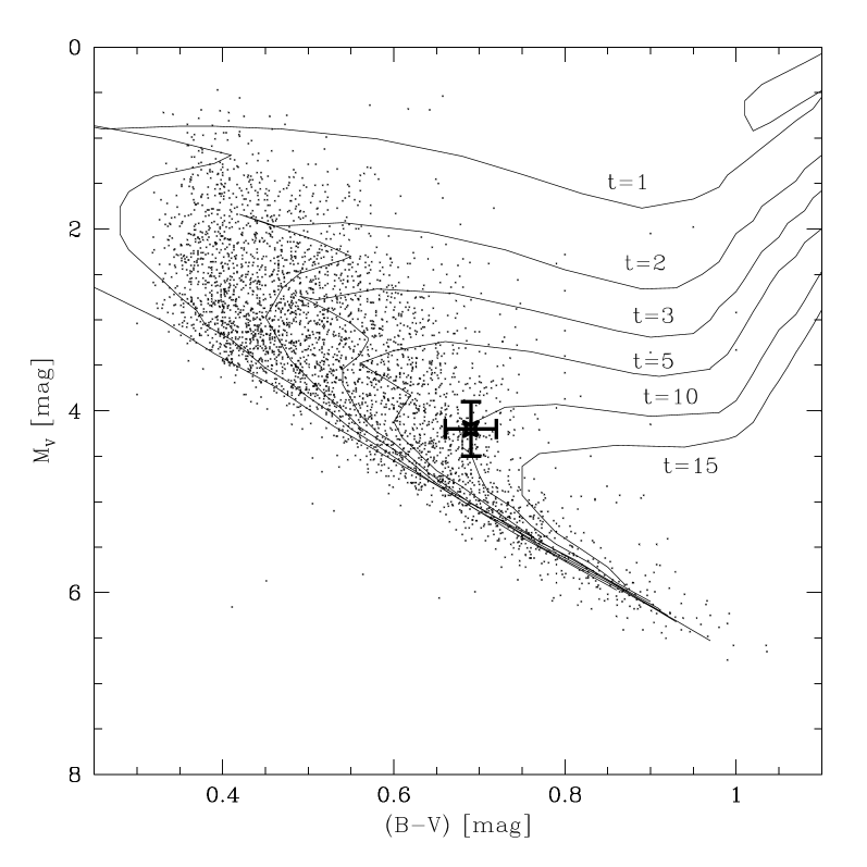
Figure 1: Representative example of a colour-magnitude diagram for dwarfs in the solar neighbourhood (from GCS) with metallicities near solar. The isochrones from Girardi et al. (2000) for z=0.02 are overlaid. Typical observational uncertainties are illustrated for one data point in the post-main sequence zone. The age probability distributions for this point are given in the lower panel. Dashed line: Gaussian distribution with 10$\pm 2$ Gyr. Dotted line: likelihood pdf for the sample point. Solid line: posterior age pdf.

2.2 Simplified 1-D approach

By reducing the dimensionality of the problem, we can illustrate some fundamental statistical features of the age determination. Les us assume here that the age, $t$, is computed from a single observable parameter, the logarithm of luminosity $\log L$. The objective is to estimate the probability distribution of the real age, $t$, given the observed value $\log L_{\mbox{\scriptsize obs}}$ and the transformation law $\log L={\cal F}(t)$. This is done through Bayes’ theorem:

$$\mbox{prob}\left(t\mid\log L_{\mbox{\scriptsize obs}}\right)=\frac{\mbox{prob}(\log L_{\mbox{\scriptsize obs}}\mid t)}{\mbox{prob}(\log L_{\mbox{\scriptsize obs}})}\mbox{prob}(t)$$

Without prior knowledge on the real age, we assume that the prior probability $\mbox{prob}(t)$ has a flat distribution between $0$ and $t_{\mbox{\scriptsize max}}$. The difficulty is that the likelihood is expressed in the parameters of the observables, while the prior is expressed in terms of the physical parameter $t$. Since Bayes’ theorem has to be expressed in a coherent set of variables, the probability distribution functions have to be modified accordingly (using the transformation ${\cal F}$). In one dimension, this is done by the chain rule:

$$\mbox{prob}(\log L)\,\mbox{d}\log L=\mbox{prob}(\log L)\mid\frac{\mbox{d}{\cal F}(t)}{\mbox{d}t}\mid\mbox{d}t$$

where $\mbox{prob}(\log L)$ should be expressed in the variable $t$.

An actual example of the transformation between $t$ and $\log L$ is shown in Fig. 2. The ${\cal F}$ relation at solar temperature and metallicity can be approximated by two linear relations with a strong change of slope at the end of the main sequence:

$$\log L={\cal F}(t)=\left\{\begin{array}[]{ll}\alpha t+\gamma&\mbox{if $0<t\leq t_{0}$}\\ \beta(t-t_{0})+\alpha t_{0}+\gamma&\mbox{if $t_{0}<t<t_{\mbox{\tiny max}}$}\end{array}\right.$$

with $\beta\gg\alpha$. In our example, $\alpha=0.015$, $\beta=0.15$, $\gamma=-0.058$, $t_{0}=9.2$ Gyr and $t_{\mbox{\tiny max}}=11$ Gyr.

We further assume that the noise measurement on $\log L$ has a Gaussian probability distribution with standard deviation $\sigma_{\log L}$.

In this case the likelihood is expressed as:

$$\mbox{prob}(\log L_{\mbox{\tiny obs}}\mid\log L)=\frac{1}{\sigma_{\tiny\log L}\,\sqrt{2\pi}}\exp-\frac{(\log L_{\mbox{\tiny obs}}-\log L)^{2}}{2\sigma_{\tiny\log L}^{2}}$$

The uniform prior probability distribution of the age $t$ is transformed, using the chain rule, into the prior probability distribution expressed in $\log L$:

$$\mbox{prob}(\log L)=\left\{\begin{array}[]{ll}c_{1}&\mbox{if $\log L\leq\log L_{0}$}\\ c_{2}&\mbox{if $\log L>\log L_{0}$}\end{array}\right.$$

With $c_{1}=(\beta/\alpha)c2$ and $\log L_{0}={\cal F}(t_{0})$. The prior expressed in $\log L$ is therefore a step function.

Figure 2: Solid line: Transformation law ${\cal F}$, $\log L={\cal F}(t)$, i.e. the logarithm of the luminosity, $\log L$, as function of the age, $t$, at fixed solar temperature (5780 K) from Geneva stellar evolution models (Schaller et al. 1992). Dashed line: simple modelisation of ${\cal F}$ in two regimes. The slope of ${\cal F}$, low below 9.2 Gyr (main-sequence phase), becomes much higher above 9.2 Gyr (evolved phase). The ratio between the speed of evolution (ratio of the slopes) is about a factor 10.

Figure 3: Upper panel: Prior of uniform age (dotted line), likelihood (dashed) and posterior (solid line) probability distribution functions, all expressed in $\log L$. Lower panel: Prior (dotted line), likelihood (dashed line) and posterior probability distribution (solid line) functions expressed in age.

Finally, the posterior pdf can be expressed in the age variable, $t$:

$$\begin{array}[]{l}\mbox{prob}(t|t_{\mbox{\tiny obs}})=\\ \\ \left\{\begin{array}[]{ll}\sim\frac{\alpha c1}{\sigma\sqrt{2\pi}}\exp-\frac{(\alpha t+\gamma-\log L_{\mbox{\scriptsize obs}})^{2}}{2\sigma^{2}}&\mbox{if $0<t\leq t_{0}$}\\ \sim\frac{\beta c2}{\sigma\sqrt{2\pi}}\exp-\frac{(\beta(t-t_{0})+\alpha t_{0}+\gamma-\log L_{\mbox{\tiny obs}})^{2}}{2\sigma^{2}}&\mbox{if $t_{0}<t<t_{\mbox{\tiny max}}$}\\ 0&\mbox{otherwise}\end{array}\right.\end{array}$$

where $\sigma=\sigma_{\log L_{\mbox{\scriptsize obs}}}$.

Let us consider a measurement obtained at the value $\log L_{obs}$=${\cal F}(t\!=\!8.5$ Gyr). Fig. 3 shows the corresponding prior, likelihood and posterior probability distributions in terms of $\log L$ and of $t$.

Several effects are apparent:

1. The transformation laws ${\cal F}^{-1}(\log L)$ and ${\cal F}(t)$ can qualitatively modify the probability distributions. Even if the likelihood pdf has a Gaussian shape in the variable $\log L$, it can be drastically different when expressed in age.

2. In the literature, the quoted $\sigma_{-},\sigma_{+}$ around the estimated age are often the simple transformation of the two values $mean_{\log L}-\sigma_{\log L}$ and $mean_{\log L}+\sigma_{\log L}$ of the likelihood function through ${\cal F}^{-1}$. These are not necessarily directly related to the quantiles or standard deviation of the posterior age pdf. The posterior pdf may have a non-Gaussian shape, its mean value, moments and quantiles may be all modified by the prior and by the transformation law ${\cal F}$. In the example of Fig. 3 the posterior pdf has become very asymmetric.

3. The prior pdf expressed in the variable $\log L$ is unevenly distributed, with a lower probability for $\log L$ for ages higher than 9.2 Gyr. This results in a strong decrease of the posterior pdf compared to the likelihood for ages higher than 9.2 (see below).

In this 1-D model, ages that are not calculated though Bayes’ theorem are subject to a systematic bias that we call the ”terminal age bias”. ”Terminal age” refers to the age for which the ${\cal F}$ relation changes slope, roughly corresponding to the end-of-main-sequence lifetime. Fig. 4 illustrates this bias by plotting the age ${\cal F}^{-1}(\log L)$ against the real age for a randomly drawn sample with $0<t<t_{max}$. The histogram of the likelihood ages is given for the real age interval $6<t<7$, showing the strong excess of the likelihood ages near the terminal age.

Figure 4: (a) Uniform random sample of true ages, as a function of the age determined with the direct method ${\cal F}$${}^{-1}(\log L)$. The discontinuity of the distribution of ages is clearly visible at the age corresponding to the end of the main sequence. We call this phenomenon the terminal age bias. (b) Histogram of ages from the direct method with true ages between 6 and 7 Gyr, as indicated in (a).

The biased nature of the likelihood-based method is apparent. Maximum likelihood gives the ”best” solution in the sense of taking the most probable value of the likelihood function. However, it does not take into account the fact that some values of $\log L$ are more likely a priori due to the shape of the ${\cal F}$ function, in our example that contamination from the slower-evolving main-sequence is important in the subgiant zone.

When using a maximum likelihood method, systematic biases have to be evaluated with additional Monte-Carlo simulations, and the estimator corrected if necessary. Additional knowledge of the system that was not used to compute the statistical estimator is added in the Monte-Carlo simulations.

Bayesian methods take a more direct approach by integrating all the knowledge about the system in the posterior pdf. This makes the results sensitive to the underlying assumptions, but removes strong systematic biases from the posterior pdf.

2.3 Extension to 3-D and Monte Carlo integration

We can now extend the previous discussion from 1 to 3 dimensions. Let us consider again the stellar evolution models as a function ${\cal F}$ relating the ”physical” parameters $\mbox{\boldmath$X$}\equiv(m,t,z)$ to the ”observational” parameters $\mbox{\boldmath$Y$}\equiv(T,L,[\textrm{Fe/H}])$, with three components:

$$\mbox{\boldmath$Y$}={\cal F}(\mbox{\boldmath$X$})\Leftrightarrow\left\{\begin{array}[]{r c l}T&=&{\cal F}_{T}(m,t,z)\\ L&=&{\cal F}_{L}(m,t,z)\\ [\textrm{Fe/H}]&=&\log(z/z_{0})\\ \end{array}\right.$$

Given an observed data triplet,

$$\mbox{\boldmath$Y$}_{o}\equiv(T_{\mbox{\scriptsize obs}},L_{\mbox{\scriptsize obs}},[Fe/H]_{\mbox{\scriptsize obs}})$$

we want to calculate the conditional probability of $X$, $\mbox{prob}(\mbox{\boldmath$X$}|\mbox{\boldmath$Y$}_{o})$, in particular the age conditional probability $\mbox{prob}(a|\mbox{\boldmath$Y$}_{o})$ for all possible ages $a$.

According to Bayes’ theorem:

$$\mbox{prob}(\mbox{\boldmath$X$}\mid\mbox{\boldmath$Y$}_{o})\sim\mbox{prob}(\mbox{\boldmath$X$})\cdot\mbox{prob}(\mbox{\boldmath$Y$}_{o}\mid\mbox{\boldmath$X$})$$

Using the marginalization theorem, we integrate over mass and metallicity, to find the probability that the real age is equal to a given value $t_{0}$:

$$\mbox{prob}(t_{0}|\mbox{\boldmath$Y$}_{o})\sim\int\!\!\!\int_{R(t=t_{0})}\mbox{prob}(\mbox{\boldmath$X$})\mbox{prob}(\mbox{\boldmath$Y$}_{o}|\mbox{\boldmath$X$})\,\mbox{d}m\,\mbox{d}z$$ (3)

where the integral is done over the region $R$ defined in the $(m,t,z)$ space by the condition $t=t_{0}$.

prob($\mbox{\boldmath$Y$}_{o}\mid\mbox{\boldmath$X$}$) is the likelihood, ${\cal L}(\mbox{\boldmath$Y$}_{o},{\cal F}(\mbox{\boldmath$X$}))$. For instance, if the uncertainties on the observed parameters are Gaussian with dispersions $\sigma_{\tiny\log T}$, $\sigma_{\tiny\log L}$ and $\sigma_{\tiny[Fe/H]}$, then the likelihood would be as in Eq. 1, with $(T,L,[\textrm{Fe/H}])={\cal F}(m,t,z)$.

The term $\mbox{prob}(\mbox{\boldmath$X$})$ is the prior probability distribution. It is the distribution expected for the parameters a priori, in terms of $m$, $t$ and $z$. It can also be thought of as the density in the $(m,t,z)$ space of an imaginary parent sample, and we shall therefore note this term like a density, $\rho(\mbox{\boldmath$X$})$.

In order to compute the integral (3), the likelihood must be expressed in terms of $(m,t,z)$. The change of variable from $(T,L,[Fe/H])$ to $(m,t,z)$ is more complex than in the one-dimensional case and involves the Jacobian determinant of ${\cal F}$:

$$J=\left|\begin{array}[]{ccc}\partial{\cal F}_{T}/\partial t&\partial{\cal F}_{T}/\partial m&\partial{\cal F}_{T}/\partial z\\ \partial{\cal F}_{L}/\partial t&\partial{\cal F}_{L}/\partial m&\partial{\cal F}_{L}/\partial z\\ \partial{\cal F}_{[Fe/H]}/\partial t&\partial{\cal F}_{[Fe/H]}/\partial m&\partial{\cal F}_{[Fe/H]}/\partial z\\ \end{array}\right|$$

Then,

$$\mbox{prob}(t_{0}|\mbox{\boldmath$Y$}_{o})\sim\int\!\!\!\int_{R(t=t_{0})}\rho(\mbox{\boldmath$X$})\,{\cal L}(\mbox{\boldmath$Y$}_{o},{\cal F}(\mbox{\boldmath$X$}))\,J(\mbox{\boldmath$X$})\,\mbox{d}m\,\mbox{d}z$$ (4)

In practice, evaluating the Jacobian of the ${\cal F}$ function at all points of the 3-dimensional parameter space is a very time-consuming operation.

Integral (4) can be evaluated much more easily by Monte Carlo integration, which makes the change of variable unnecessary. In practice, only this approach can ensure results within realistic computation times for the full 3-dimensional model.

A large sample of $(m,t,z)$ triplets can be drawn following the density $\rho(m,t,z)$, then the likelihood is computed for all triplets, and the results collected in age bins, i.e.

$$\mbox{prob}(t_{0}\mid\mbox{\boldmath$Y$}_{o})\mbox{d}t\sim\sum_{t_{0}-dt/2<t<t_{0}+dt/2}{\cal L}(\mbox{\boldmath$Y$}_{o},{\cal F}(m,t,z))$$

This method has the considerable advantage of requiring no inversion or differentiation of the ${\cal F}$ function, which is difficult and subject to many numerical instabilities, and is even undefined in many regions of parameter space (where stellar evolution tracks overlap and where no track passes) and of making the change of variable from $(m,t,z)$ to $([\textrm{Fe/H}],T,L)$ easy. It also allows great flexibility as to the assumptions on the prior. For instance, the inclusion of potential binarity becomes straightforward (see Section 3.3). Another advantage is that building a random sampling of the $\rho(m,t,z)$ density is equivalent to the more familiar procedure of generating a synthetic stellar population, so that existing algorithms designed for this latter task can be used.

3 PRACTICAL APPLICATIONS

3.1 Realistic expressions for the likelihood

For simplicity, we have made up to now the unrealistic assumption of Gaussian uncertainties on temperature and luminosity. In practice, the likelihood can be expressed with suitable assumptions on the distribution of the uncertainties on the colour, magnitude, logarithmic temperature or trigonometric parallax. For instance, one can assume Gaussian uncertainties on $\log T$, $[Fe/H]$ and the parallax $\varpi$. In that case the likelihood becomes

$${\cal L}(T_{obs},\varpi_{obs},[\textrm{Fe/H}]_{obs},m,t,z)=$$

$$\frac{1}{\sigma_{[Fe/H]}\sigma_{\varpi}\sigma_{\log T}(2\pi)^{3/2}}\exp-\frac{(\log T_{obs}-\log{\cal F}_{T}(m,t,z))^{2}}{2\sigma_{\log T}^{2}}$$

$$\times\exp-\frac{({\varpi}_{obs}-10^{V_{obs}+2.5\log{\cal F}_{V}(m,t,z)/5+1})^{2}}{2\sigma_{\varpi}^{2}}$$

$$\times\exp-\frac{([\textrm{Fe/H}]_{obs}-\log\frac{z}{z_{0}})^{2}}{2\sigma_{[Fe/H]}^{2}}$$

where $V$ the visual magnitude, and ${\cal F}_{V}$ the magnitude predicted from the stellar evolution models.

3.2 Choosing a prior

Let us now build a realistic prior for the specific case of the solar neighbourhood. The prior distributions of $m$, $t$ and $z$ are assumed to be independent, i.e., no prior information is assumed on an age-metallicity relation, or on a time variation of the mass distribution. In that case, the mass, age and metallicity prior can be considered separately:

$$\mbox{prob}(\mbox{\boldmath$Y$})=\mbox{prob}(m)\cdot\mbox{prob}(t)\cdot\mbox{prob}(z)$$

The mass prior

The mass prior can be chosen as one’s favourite initial mass functions (IMF) derived for the Galaxy. Within reasonable limits, the precise choice of IMF will not have a strong influence, because the mass range covered by the F and G dwarfs is not large.

The age prior

The age prior is the expected age distribution of all stars ever born in the sample considered (the fact that some of them have already died is accounted for in the ${\cal F}$ function), in other words the star formation rate (SFR) of the sample considered. The SFR of the Galactic disc is not precisely known. It seems to have been globally constant or slightly decreasing (Hernandez, Valls-Gabaud & Gilmore 2000; Chang, Shu & Hou 2002; Vergely et al. 2002), but its small-scale structure is still largely unknown. At this stage a flat age prior is a reasonable assumption. Decreasing priors can also be used. Within reasonable limits, the slope of the SFR does not make large differences in the recovered age pdfs.

Note that using a flat age prior is not at all equivalent to ignoring the age prior. A flat prior in age is far from translating into a flat prior in parameter space (see Section 2.1). Fig. 5 shows the prior distribution of magnitude at solar values of temperature and metallicity resulting from a flat age prior. The abrupt slope towards bright magnitudes is due to the acceleration of evolution in temperature and magnitude after the main-sequence phase. The cutoff at faint magnitudes is obviously due to the absence of models below the zero-age main-sequence.

For a flat or slightly decreasing age prior, an upper age cutoff must be chosen. This somewhat arbitrary procedure has a direct influence in the derived age distribution by simply removing all ages above the cutoff. At present, the maximum age of the stars in the Galactic disc is not well known. The age of the thin disc has been studied by Binney et al. (2000), but the solar neighbourhood also contains thick disc stars, whose age may be several Gyr higher than that of the oldest thin disc stars.

Figure 5: Magnitude probability distribution corresponding to a flat age prior, with $\log T=3.76$ and $[\textrm{Fe/H}]=0.0$. The sharp shape is due to the highly non-linear nature of the function ${\cal F}_{L}(m,t,z)$.

The metallicity prior

In the case of the Galactic disc, a good metallicity prior is the expected distribution of a volume-limited sample of the solar neighbourhood. Two such distributions are displayed on Fig. 6. The influence of the metallicity prior depends on the size of the observational uncertainties on $[\textrm{Fe/H}]$. For very high accuracy spectroscopic metallicities, with $\sigma_{[Fe/H]}\simeq 0.05$ dex (e.g. E93), the likelihood is narrow enough to overwhelm the changes in the prior. For uncertainties most typical of larger surveys and of photometric metallicities, $\sigma_{[Fe/H]}\simeq 0.10$ dex, the influence of the prior becomes more significant, especially in the regions where it is varying more rapidly: at the high-metallicity end and at the connection between the main thin-disc distribution and the thick-disc tail near $[\textrm{Fe/H}]\simeq-0.5$. The systematic bias on likelihood-based methods can reach 0.1 dex in metallicity, causing systematic biases on the derived ages.

When the metallicity uncertainty $\sigma_{[Fe/H]}$ is even higher, for instance when collecting metallicities from different calibrations (e.g. Ibukiyama & Arimoto 2002, with $\sigma_{[Fe/H]}\sim 0.15$ dex), the influence of the metallicity prior will become so important that the derived ages will be highly dependent on it and extremely uncertain. Maximum likelihood ages will be strongly biased, and will produce visibly unreliable results such as fig. 5 of Ibukiyama & Arimoto (2002). It is apparent from our Fig. 6 that $\sigma_{[Fe/H]}\sim 0.15$ implies that the variation of the likelihood will not be steeper than the variation of the prior, which is the Bayesian definition of a ”bad measurement”.

Figure 6: Metallicity distribution for the solar neighbourhood and metallicity prior. Stars: G-dwarf volume-limited metallicity distribution according to Jørgensen (2000). Dotted line: Metallicity distribution of the GCS survey. Dashed line: Metallicity prior adopted in the present paper. Insert: Gaussian probability distributions corresponding to dispersions $\sigma_{[Fe/H]}=$0.05, 0.10 and 0.15 dex.

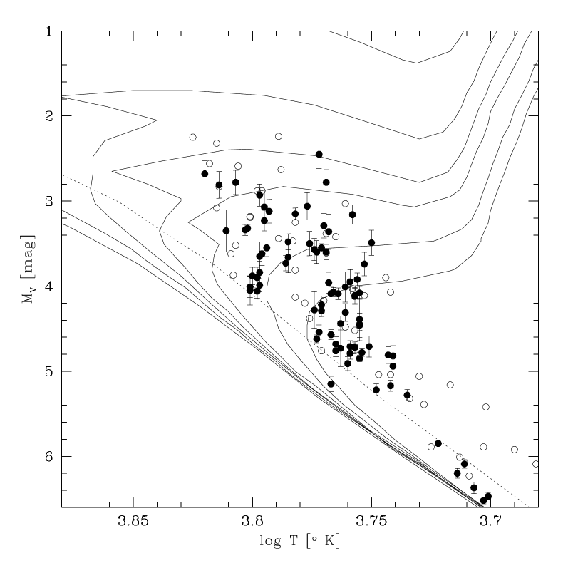
Figure 7: Theoretical isochrones from the Padua models for $[\textrm{Fe/H}]=-0.7$ (0,1,2,3,5,10 and 15 Gyr) and objects in the GCS catalogue with $-0.75<[\textrm{Fe/H}]<-0.65$. Detected binaries are indicated with open symbols. The error bars show the uncertainties due to the parallax. The dashed line is the solar-metallicity ZAMS. Part of the obvious temperature mismatch between models and observations may be due to the slope of the metallicity prior. Taking the models and observations at face value would lead to assigning terminal ages to practically all stars.

3.3 Accounting for undetected binaries

Up to this point, we have considered that all stars in our sample obeyed the ${\cal F}$ relation between $(m,t,z)$ and $(T,L,[\textrm{Fe/H}])$ with Gaussian uncertainty distributions. Even without considering such second-order effects as rotation or Helium abundance, this relation does not always hold for real stars, particularly in the case of undetected binaries. The light from the companion of an undetected binary can move a given object up to 0.75 mag (for equal-mass binaries) above its true position in the colour-magnitude diagram. This obviously has a profound effect on the age determination.

If the number of undetected binaries in the sample is not too large, its effect on the age determination for main-sequence stars will be manageable. A few of the ages will turn out to be overestimated.

The effect of the binaries on the age determination of evolved stars in the subgiant zone, however, will be large. Because the evolution is more rapid in the subgiant zone, the probability of finding a star in a subgiant stage is much lower than for the main-sequence stage. On the other hand, undetected binarity can move main-sequence objects upwards into the subgiant zone of the $(T,L)$ plane. As a result, the contamination of binaries in the subgiant zone can be very important.

The standard approach to the age determination offers no obvious way to deal with the binary contamination, which has to be treated as a nuisance and studied with separate simulations.

In the Bayesian formulation, the inclusion of undetected binaries is not particularly difficult. A term can be added to equation (3) integrating the hypothesis that the object can be an undetected binary:

$$\mbox{prob}(t|\mbox{\boldmath$Y$}_{o})\sim\mbox{prob}(t)\cdot\mbox{prob}(\mbox{\boldmath$Y$}_{o}|\textrm{{single or binary}, t})$$

Because binarity and non-binarity are mutually exclusive, the probability sum rule can be used to yield:

$$\mbox{prob}(t|\mbox{\boldmath$Y$}_{o})\sim\mbox{prob}(t,\textrm{single})\mbox{prob}(\mbox{\boldmath$Y$}_{o}|t,\textrm{single})$$

$$+\mbox{prob}(t,\textrm{binary})\mbox{prob}(\mbox{\boldmath$Y$}_{o}|t,\textrm{binary})$$

If age and binarity are independent, then

$$\mbox{prob}(t|\mbox{\boldmath$Y$}_{o})\sim\mbox{prob}(t)(\mbox{prob}(\mbox{\boldmath$Y$}_{o}|t,\textrm{single})+q\,\mbox{prob}(\mbox{\boldmath$Y$}_{o}|t,\textrm{binary}))$$

where $q\equiv\mbox{prob}(\textrm{binary})/\mbox{prob}(\textrm{single})$ is the rate of undetected binaries.

In practice, because binarity has such a large effect on the age determination, one may be less interested in knowing the age pdf in the case of binarity than to know the total probability for the star to be a binary, ”$\mbox{prob}(\textrm{binary}\mid\mbox{\boldmath$Y$}_{0})$”. To calculate this probability, we integrate over all values of $t$:

$$P_{bin}\equiv\mbox{prob}(\textrm{binary}|\mbox{\boldmath$Y$}_{o})=$$

$$\int\mbox{prob}(\textrm{binary},t|\mbox{\boldmath$Y$}_{o})\mbox{d}t=$$

$$q\int\mbox{prob}(t)\mbox{prob}(\mbox{\boldmath$Y$}_{o}|t,\textrm{binary})\mbox{d}t$$

The terms inside the integral can be calculated as in Section 2, using the modified relation ${\cal F^{\prime}}$ between $(m,t,z)$ and ($T,L,[\textrm{Fe/H}]$) suitable for binaries, depending on the mass ratio parameter.

The computations show that $P_{\mbox{\scriptsize bin}}$ is small in some parts of the $(T,L)$ plane and much larger in others, particularly 0.75 mag above the main-sequence, as could be expected. At that position, it reaches about 10 times the value of $q$ (implying that for an undetected binary rate of 10 percent, the object is actually as likely to be a binary as a single star). The interesting thing is that the Bayesian computation not only yields a specific value of $P_{\mbox{\scriptsize bin}}$ for each object for any subsequent statistical study, but also includes in the posterior age pdf the possibility of the star being an undetected binary. In this way, undetected binaries are less likely to introduce unrecognized contamination in the scientific analysis of the results (see Section 5).

3.4 Choice of stellar evolution models and temperature scale match

Sets of stellar evolution tracks for late-type dwarfs have been produced by many different groups. Some of the most widely used are Girardi et al. (2000), Yi et al. (2001), Lejeune & Schaerer (2001). The agreement between the predicted isochrones from the different groups is generally good on or near the main sequence, so that using one set of models rather than another doesn’t introduce dramatic differences in the derived stellar ages. Two robust predictions of stellar evolution theory, that heavier stars evolve more quickly and that stars on the main sequence get brighter with age, provide the dominant tendencies.

There are, however, important residual differences between the sets of models, that have a significant influence on the age determination. Of particular importance are the known difficulties related to the model temperature predictions: absolute temperature scale of the models, colour-temperature conversions, metallicity dependence of the position of the unevolved main sequence. There also are significant systematic differences between the model temperature predictions and the observed position of well-measured field dwarfs (Lebreton et al. 1999; Lebreton 2000; Kotoneva et al. 2002b).

As far as the age determination is concerned, the important fact is that the models and observations be on the same relative temperature scale. The observation of nearby unevolved K-dwarf stars with well-known parallaxes and metallicities shows that the actual colour change with metallicity is significantly lower than model predictions (Kotoneva et al. 2002b). Several explanations have been proposed for this mismatch, including problems with the temperature-colour conversions, metallicity-dependent helium abundances, and heavy-element sedimentation (Lebreton et al. 1999). None of these effects seems able to account for the whole mismatch. Some moderately metal-deficient dwarfs in the solar neighbourhood are compared with model predictions in Fig. 7 to illustrate the amplitude of the mismatch between the Girardi et al. (2000) models and the observations. Obviously, ages derived with such a large temperature mismatch will be strongly biased towards terminal ages.

Several schemes can be adopted to ensure that the models and observations are coherent, either at the level of the colour-temperature conversion, or as empirical temperature shifts in the models.

PART TWO: Application to the E93 sample and the age-metallicity relation

4 Bayesian ages for the E93 sample and solar neighbourhood AMR

In this Section, we apply the Bayesian age calculation to a specific case, the landmark E93 study (see Introduction). As an illustration and important application of the approach developed in the previous sections, we calculate the posterior age pdf for the objects of the E93 sample, and reconsider their determination of the age-metallicity relation of the Galactic disc.

4.1 Recent data for the E93 sample

The E93 sample was selected from the large Olsen (1994) catalogue of F and G dwarfs in the solar neighbourhood. The selection criteria were approximately a range in temperature, $5600<T<6800$, and in evolution away from the Zero-Age Main Sequence, $M_{V}-M_{V,ZAMS}>0.4$ mag. The objective was to select stars in the subgiant portion of the CMD, where the isochrones are more widely spaced and age determinations are presumably more accurate.

The main emphasis of E93 was on providing accurate metallicities. They estimated the relative accuracy of their metallicities to be 0.05 dex. They derived ages for their objects by comparison with Vandenberg (1985) isochrones. The adopted ages were that of the isochrone crossing the position of the data in the temperature-luminosity plane. The uncertainties on the ages were estimated to be around 0.1 dex, based on the direct propagation of the observational errors. In our notation, E93 have computed age estimates from

$$t={\cal F}^{-1}(T,L,[\textrm{Fe/H}])$$

and evaluated the uncertainties with

$${\cal F}^{-1}(T\pm\sigma_{T},L\pm\sigma_{L},[\textrm{Fe/H}]\pm\sigma_{[Fe/H]})$$

E93 provide evidence for the 0.1 dex value of the age uncertainties by displaying data for M67 and showing that, indeed, the dispersion of the inferred ages is of the expected order, at least in the subgiant portion of the CMD.

The data for all E93 objects have been significantly improved in the intervening decade, the only exception being the individual metallicities, that were of high relative accuracy in E93. The most noteworthy addition is the availability of Hipparcos parallaxes, that allow the distances – hence the absolute magnitudes – of the objects to be known with much better accuracy than was available to E93. Most stars in the sample have distances of less than 50 pc, and correspondingly uncertainties of less than 5 percent in the Hipparcos parallaxes, in contrast with the 14 percent uncertainty assumed by E93 for the photometric distances.

The second important addition to the E93 data is that of further radial velocity monitoring (GCS), that has revealed a certain number of spectroscopic binaries.

Ng & Bertelli (1998) have reconsidered the E93 sample with Hipparcos distances, and with the Bertelli et al. (1994) stellar evolution models. However, their age derivation method is not fundamentally different from E93, and they consequently derive a similar age-metallicity plot. It is already apparent in their study, though, that the new distances considerably reduce the number of stars in the high-metallicity, high-age section of the diagram. This could be expected, because it is precisely in this region, the terminal-age subgiant region, that objects get preferentially scattered by the distance errors (see Section 2.2). It is also worth noting that many stars are put back on the main-sequence with $\Delta M_{V}<0.4$ by the new distances, proving the reality of the biases associated with the non-Bayesian calculation.

Another valuable improvement was brought by Lachaume et al. (1999), who computed the distribution of the likelihood for the age estimation of a sample of 91 local field dwarf stars. While this still ignores the prior pdf, it does show that the 1-$\sigma$ interval for the derived ages is larger than 0.1 dex for many objects in the crucial 3-10 Gyr range.

Finally, the Hipparcos data have also allowed the discovery of large temperature shifts between models and data (see Section 3.4), that were not corrected by E93 or Ng & Bertelli (1998) and also affect the age determinations.

4.2 Bayesian ages for the E93 sample

Posterior age pdf’s were computed for the objects in the E93 sample using the method of Section 2.3. The age prior is taken as flat, with a cutoff at $t_{max}=15$ Gyr, the mass prior as a power function of slope $-2.35$. The metallicity prior is a Gaussian centered on $[\textrm{Fe/H}]=-0.15$ with a dispersion of 0.19 above $[\textrm{Fe/H}]=-0.53$, and a constant below $[\textrm{Fe/H}]=-0.53$ with a cutoff at $[\textrm{Fe/H}]=-1.0$ (see Fig. 6). This function is a visual approximation of the metallicity distribution of the whole GCS, and is also compatible with the volume-limited distribution for the solar neighbourhood derived by Jørgensen (2000). The stellar population synthesis code IAC-star (Aparicio & Gallart 2004) was used for the Monte-Carlo estimation of $\rho(m,t,z)$ and the ${\cal F}$ transformation. The E93 metallicities were put on the scale of Santos et al. (2002) by a shift of +0.12 dex. The temperature scale in GCS (as of 2003) was used, adjusted by a shift of $+0.006$ to obtain a satisfactory match between the Padua isochrones and the GCS data in the theoretical plane.

Gaussian uncertainties were assumed on $[\textrm{Fe/H}]$, $\log T$ and $M_{V}$. Several different sets of values were used for the standard dispersions of the uncertainties. See Section 5 for a confrontation of different cases. For our ”standard” computation, we used $\sigma_{\log T}=0.009$ $\sigma_{Mv}=0.15$ and $\sigma_{[Fe/H]}=0.075$. We arrive at these values by using the uncertainties proposed by Ng & Bertelli for their revision of the E93 sample ($\sigma_{[Fe/H]}=0.05$, $\sigma_{\log T}=0.006$), an $M_{V}$ uncertainty of 0.10 mag (5 percent uncertainty on the distance), and allowing for the possible presence of systematic errors of similar amplitude by multiplying all values by a factor 1.5. It is important to remember that differences such as a zero-point shift in the metallicity scale or temperature scale have a strongly non-linear effect on the age determination (i.e. shifting the temperature scale does not produce a single shift of all age values but very different shifts depending on the position in the CMD). Systematic zero-point differences of 0.10 dex in $[\textrm{Fe/H}]$ and 0.005 in $\log T$ are common between different scales. Indeed, as mentioned above, shifts of such magnitude were found necessary to match the theoretical isochrones with the observational data. The use of $[\textrm{Fe/H}]$ itself as a surrogate for the total heavy-element abundance used in the theoretical models is also subject to uncertainties, given the observed variations in the abundance ratios from star to star. In the Bayesian treatment, these sources of error have to be integrated into the assumed observational uncertainties. It is crucial to use the real difference between the data and the evolution tracks to estimate the likelihood, not the relative difference.

Figure 8: Posterior age pdf, between 0 and 15 Gyr, for representative late-type examples of the updated E93 data. The dotted line indicates a Gaussian of 0.1 dex dispersion around the E93 age value, for comparison.

Fig. 8 gives posterior age pdf for a few representative objects in the sample, compared with a 25 percent ($\sim 0.1$ dex) dispersion Gaussian centered on the E93 age estimate. The results show that the shape and width of the posterior age pdf can vary a lot from one star to the next. Both the central value and the general shape of the posterior probability distributions of the age are often very different from that obtained by E93 with the ${\cal F}^{-1}$ approach. In some cases, a Gaussian is a valid approximation, but many stars are subject to wider and very asymmetrical probability distributions. Some have posterior pdf spanning most of the allowed 0-15 Gyr range, so that the chosen age value is sensitively dependent on the assumed prior. In these cases, the derived age is not well determined (e.g. HD 115617, HD 177565, HD 98553 in the Figure).

4.3 Age-metallicity relation

Figure 9: a The original age-metallicity plot from E93. b the age-metallicity plot for the E93 sample with new data: luminosities from Hipparcos distances, temperatures from GCS, ages from the present study. Symbols as follows: crosses–binary in the GCS catalogue, open circles–photometric distance from E93 discrepant with Hipparcos distances by more than 20 percent, metallicity from E93 and from GCS by more than 0.2 dex, or temperature/colour discrepant between E93 and GCS. c The age-metallicity relations used in the Bayesian models of Section 5. d Simulated age-metallicity plot, resulting from an age-metallicity relation of total range $\Delta[Fe/H]=0.4$ dex, and observational uncertainties $\sigma_{[Fe/H]}=0.05$, $\sigma_{T}=75$ K, $\sigma_{M_{V}}=0.15$ mag, systematic shifts 0.12 dex in metallicity and +0.005 in $\log T$. In the two top plots, the dashed lines outline two regions that are important for the evaluation of the dispersion of the age-metallicity relation, and where contamination from biased low-accuracy ages is expected to be significant (see text). ”Region I” near solar metallicity, age$>5$ Gyr, ”Region II” metal-poor, age$<6$ Gyr.

Fig. 9b plots the Bayesian ages, with the updated data, in the age-metallicity plane, using the median of the posterior pdf as an age estimator. The binaries identified in GCS are indicated as crosses.

Given the sensitivity of the age determination to the input parameters, it is important to use all the available information to identify possible outliers. The metallicities of E93 were confronted with the photometric metallicities derived in GCS, the Hipparcos parallax distances with the distances derived from the photometric calibrations in GCS. The following conditions were required for inclusion in the final sample:

$$\mid[\textrm{Fe/H}]_{E93}-[\textrm{Fe/H}]_{GCS}\mid<0.2$$

$$\mid\frac{r_{E93}-r_{GCS}}{r_{E93}}\mid<0.2$$

where $r$ is the distance. HD 67228, 112164, 199960 and 207978 were identified visually as outliers on a comparison of temperatures between E93 and GCS, and of colour between the Strömgren $(b-y)$ and Hipparcos $(B-V)$.

The objects singled out by the conditions above are indicated by open symbols in Fig. 9b. The data discrepancy indicates that they can be peculiar in some way, or that some of their measurements may be statistical outliers, so that the age determination may be affected.

Fig. 9a repeats the original E93 age-metallicity plot, for comparison. Two regions particularly important in giving an impression of high dispersion in the age-metallicity relation, and particularly prone to contamination by skewed probability distributions of age with large error bars (see Section 2.3), are indicated with dashed lines (Similar regions in the age-metallicity plot were previously used by Rocha-Pinto et al. 2000 to show that ages from chromospheric activity did not produce a high intrinsic dispersion in the AMR). The presence of many stars in these two regions in E93 contributed strongly to the conclusion of a very wide metallicity dispersion at all intermediate ages.

4.4 Discussion

Figure 10: Median Bayesian age in the age-metallicity plot for our selection of the E93 sample. For a few objects, the full-width-half-maximum and the full width at tenth maximum of the posterior age pdf are indicated. The solid and dashed lines indicate respectively the mean and envelope AMR used for Fig. 11.

Fig. 9 offers a spectacular confirmation of the effect of biases and of the potential perils of replacing the complete posterior pdf by a single maximum-likelihood point in the age-metallicity plot. Indeed, the new data give a strong indication that there were many objects in the high-age, high-metallicity part of the original E93 AMR plot that had been displaced in the subgiant zone by high observational uncertainties and binarity (”terminal age bias”, in our terminology). The upper dashed zone in the AMR becomes practically empty with the new data. All four points remaining in it are compatible with being one-sigma outliers from younger ages.

Fig. 10 displays the age-metallicity diagram for our selected objects, plotting the half-maximum and tenth-maximum intervals of the posterior age pdf for a few representative objects to give a feeling for the shape of the age pdf. Contrarily to the original E93 AMR, the updated AMR diagram outlines a definite monotonic relationship between age and metallicity for intermediate ages. Part of the scatter in the original relation is removed. A simple linear fit gives $[\textrm{Fe/H}]=-0.056\,\mbox{age}+0.011$, with a dispersion of 0.18 dex in metallicity, to be compared with 0.24 dex in E93. This value still includes the scatter introduced by the age uncertainties and by the fact that the actual AMR may not be linear. Therefore, 0.18 dex can be considered a strict upper limit for the ”cosmic scatter” in the AMR.

Using the posterior age pdf that we obtain for the E93 objects, Monte Carlo simulations of the whole procedure were carried out to determine what dispersion is expected from the observational uncertainties alone, assuming a dispersionless AMR. We find that a dispersion at fixed age $\sigma_{[Fe/H]}\simeq$0.10 is introduced around a dispersionless AMR by the observational uncertainties. By quadratically subtracting this dispersion from the value of 0.18 found in the observed AMR, we estimate the remaining intrinsic scatter, the so-called ”cosmic scatter”, to be at most 0.15 dex.

Therefore, with the improved data and detailed treatment of the age probability distribution, the E93 sample no longer indicates a very high scatter in the metallicity at a given age, or a near-absence of AMR in the intermediate age range. While still clearly distinct from a dispersionless AMR, the data indicate a rather well-defined growth of mean metallicity with time, with an intrinsic dispersion of the order of 0.15 at most.

A similar conclusion was already obtained by Rocha-Pinto et al. (2000) on the basis of chromospheric ages for solar-neighbourhood dwarfs. Their result was subsequently criticized on the basis of the observed disagreement between isochrone ages and chromospheric ages (e.g. Feltzing et al. 2001). However, the present study brings support to the validity of the indications from chromospheric ages and shows how the apparent disagreement could arise from strong systematic errors on the isochrone ages.

In the following two paragraphs, we examine other ways to look at the data that can add more indications on the reality of the high intrinsic scatter, by considering the two regions, ”Region I” and ”Region II”, that we defined in the age-metallicity diagram on Fig. 9.

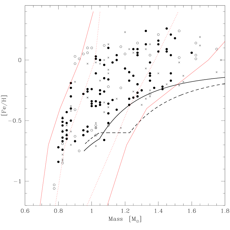
Figure 11: Mass-metallicity relation for our sample. Symbols as in Fig. 9b. The thick lines indicate the lower envelope of the mass-metallicity relation for a low-dispersion AMR (solid line in Fig. 10 with a 0.24 dex range in [Fe/H]) and high dispersion AMR (dashed line). The oblique dotted and solid lines indicate the zones affected by the temperature selection biases.

4.5 ”Region I”: solar metallicity, age $>5$ Gyr

The majority of the objects placed in or near ”Region I” of the CMD have been excluded by our quality criteria. There are five detected binaries. The other objects are stars with $M\sim 0.9M_{\odot}$, for which the Hipparcos distance is much smaller than the distance obtained by E93 from the photometry (more than 20 percent difference, these objects are HD 76151, 86728, 108309, 115617, 127334, 177565 and 217014). Because the main-sequence is narrow for $M\sim 0.9M_{\odot}$, these smaller distances, implying fainter $M_{V}$, are sufficient to bring these stars from the subgiant zone (with apparently well determined ages in the 5-10 Gyr range) back on the main sequence. These objects were therefore outliers of the Strömgren $M_{V}$ calibration that had been preferentially selected by the $\Delta M_{V}>0.4$ criteria of E93. The Hipparcos distances put them back on the main-sequence where, for such low masses, no accurate estimate of the age can be given.

This illustrates a side-effect of the $\Delta M_{V}>0.4$ selection criteria used by E93. Intended to select only stars in the region of the CMD were isochrones are well-spaced, it also samples the region of the CMD where the difference between likelihood and posterior is larger, and the proportion of undetected binaries is higher. The E93 study picked up 189 stars out of more than 19’000, and in the process it favors the 2-3 $\sigma$ outliers from the main sequence. Simple statistical considerations show that the number of main sequence contamination in the $\Delta M_{V}>0.4$ zone must be large. The Bayesian approach automatically includes this selection effect in the posterior pdf, by taking into account the prior distribution $\mbox{prob}(t)$, which is heavily weighted towards the main-sequence, and the bias caused by the selection criteria is absent in our updated sample, thanks to the fact that the Hipparcos parallaxes are used to re-compute values of $M_{V}$ that are independent of the original photometric $M_{V}$ used in the sample selection.

Note that ”Region I” is even more populated in the higher-uncertainty samples of Ibukiyama & Arimoto (2000) and Feltzing et al. (2001). The presence of many objects in this region of the age-metallicity diagram does not give any indication of the real existence of such high-metallicity, intermediate-age stars. On the contrary, the E93 sample tends to indicate that this region is actually empty, because there is not a single bone fide subgiant with an age above 7 Gyr and a metallicity near solar.

Interestingly, the Sun, at $t=4.5$ Gyr and $[\textrm{Fe/H}]$=0, seems to be near the upper edge of the compatible age-metallicity distribution of the sample (Wielen et al. 1996). This may be related to the observed statistical overabundance of planet host stars (Gonzalez 1998; Santos, Israelian & Mayor 2000).

4.6 ”Region II”: metal-poor, age $<6$ Gyr

Let us now consider the second dashed region, ”Region II”, in the low-age ($t\leq 6$ Gyr), low-metallicity ($[\textrm{Fe/H}]\leq$ 0.5) part of the diagram.

The age-metallicity diagram shows a few data points in this region that may or may not have been scattered there by the uncertainties on the age determination (for none of these objects is the whole posterior age pdf entirely contained in ”Region II”). Fortunately, there is another way to determine whether this region of the AMR is really occupied.

The age estimation from isochrones also provide an estimation of mass. The mass can be derived from theoretical tracks in a more reliable way that the age, because the mass changes relatively slowly with the observed parameters. A fundamental feature of stellar evolution is the fact that the duration of the main-sequence phase is a very sharp function of mass. This sharp dependence implies the following: only stars below a certain mass can reach ages above a given age. E.g., only stars with masses below 1.2 $M_{\odot}$ can reach ages above 5 Gyr, and masses below 1 $M_{\odot}$ ages above 10 Gyr. This relation between mass and maximum age implies that the lower envelope of the mass-metallicity relation will depend on the AMR and its dispersion. As we move to lower masses, higher ages become available and the metallicities reached at these ages begin to appear in the age-mass relation.

Therefore, if there really are low-age (3-6 Gyr), low-metallicity ($[\textrm{Fe/H}]\leq-0.5$) stars –objects within Region II– then we expect such stars to be of all masses able to reach at least 3 Gyr of age, $M<\sim 1.3M_{\odot}$. On the other hand, if Region II is not actually occupied, and the points in the age-metallicity diagram are scattered into it by the uncertainties from higher ages, then this should be revealed by the absence of $M\sim 1.1-1.3M_{\odot}$ stars with lower metallicity. The region in the mass-metallicity diagram from which low-metallicity stars start to be found gives a definite indication of the minimal age of such stars.

Fig. 11 shows the mass-metallicity plot for the E93 sample with the updated data. E93 do not give mass estimates for their stars. Masses for Fig. 11 were computed by us as a by-product of the age computation. The upper envelope of the relation between mass and maximum age was adjusted on the GCS data as $\log t_{lim}=1.09-4.35\log(mass)$. Via this relation, the lower envelope of the AMR can be converted into a lower envelope in the mass-metallicity plot. Fig. 11 gives the predicted lower envelopes of the mass-metallicity relation with the two AMR plotted in Fig. 10. The first is a $\Delta=0.24$ dex relation defined by the solid line on Fig. 10, and the second (dashed line) is the lower envelope of an AMR with very high intrinsic scatter, of the type inferred from the original E93 interpretation. The crucial difference between the two AMR is that one predicts the real existence of objects in Region II while the other does not. The zones affected by the selection biases of E93 are also indicated in Fig. 11. Selection becomes increasingly unlikely as one moves from the dotted to the solid limits.

The result definitely leans towards the absence of low-metallicity, low-age stars. Although the selection biases affect the region of interest, the observed envelope clearly favours the low-dispersion AMR model. The most significant evidence is the lack of metal-poor, 1.1-1.3 $M_{\odot}$ stars. This absence is best explained by the fact that 1.1-1.3 $M_{\odot}$ stars, with maximum ages in the 5-8 Gyr range, are too young to have experienced metallicities as low as $[\textrm{Fe/H}]=-0.6$. Consequently, the objects observed in ”Region II” in the AMR plot are lower-mass objects, scattered from higher ages by the observational error. A fact fully compatible with their age probability pdf.

This is a solid indication that the lack of definite AMR in the E93 sample is only apparent, independently of the discussion of the age probability pdf. It should be confirmed with samples with wider selection criteria and more objects, for instance by obtaining precise spectroscopic metallicities for a sample of 1.1-1.3 $M_{\odot}$ stars with a higher temperature cut.

5 The dispersion in the AMR from Bayesian model comparison

As the present study has indicated, the derivation of the AMR and its intrinsic dispersion from the age-metallicity plot is made difficult by the shape of the age uncertainties. Replacing prior-dependent age estimates with large and asymmetrical uncertainty distributions by single points makes direct ”eyeball” analysis unreliable, and does not permit the collection of the metallicity data into separate age bins.

However, this does not imply that the data cannot be used to study the AMR. The posterior age pdf contains all the information available on the ages, and there are other ways to analyse the data and constrain the dispersion of the AMR, such as the mass-metallicity relation used in Section 4.5.

The Bayesian framework also provides tools for the comparison of different models. Let us call ${\cal M}$ the model assuming a particular AMR with an intrinsic range $\Delta[\textrm{Fe/H}]$. The model consists of

• a mean age-metallicity relation: $[\textrm{Fe/H}]=f(t)$ with an intrinsic range $\Delta[Fe/H]$,

• stellar evolution models $L={\cal F}_{L}(m,t,z)$ and $T={\cal F}_{T}(m,t,z)$,

• assumptions about the distribution of the observational uncertainties (for instance Gaussian on $\log T$, $M_{V}$ and $[Fe/H]$).

What one wants to compute is $\mbox{prob}({\cal M}\mid D)$, the probability of the model ${\cal M}$ being true, given all the data $D$. In practice, one is not interested in the normalized probabilities but wishes to compare the probabilities of two models.

Using Bayes’ theorem,

$$\mbox{prob}({\cal M}\mid D)=\mbox{prob}({\cal M})\frac{\mbox{prob}(D\mid{\cal M})}{\mbox{prob}(D)}$$

the ratio of the probabilities for two models ${\cal M}_{1}$ and ${\cal M}_{2}$ is:

$$\frac{\mbox{prob}({\cal M}_{1}\mid D)}{\mbox{prob}({\cal M}_{2}\mid D)}=\frac{\mbox{prob}({\cal M}_{1})}{\mbox{prob}({\cal M}_{2})}\frac{\mbox{prob}(D\mid{\cal M}_{1})}{\mbox{prob}(D\mid{\cal M}_{2})}$$

where the unknown normalization $\mbox{prob}(D)$ vanishes in the ratio.

If the data points are independent, then the global term, ${\mbox{prob}(D\mid{\cal M})}$ can be broken down into a product of individual probabilities for the individual data points $d_{i}$.

$${\mbox{prob}(D\mid{\cal M})}=\prod_{i=1}^{N}\mbox{prob}(d_{i}|{\cal M})$$

As in Section 2.3 we marginalize over the mass and metallicity, but now also over the age:

$$\mbox{prob}(d_{i}\mid{\cal M})=\int\!\!\!\int\!\!\!\int\mbox{prob}(d_{i},m,t,z|{\cal M})\,\mbox{d}m\,\mbox{d}t\,\mbox{d}z$$

Using the probability product rule:

$$\mbox{prob}(d_{i}\mid{\cal M})=$$

$$\int\!\!\!\int\!\!\!\int\mbox{prob}(d_{i}|{\cal M},m,t,z)\,\mbox{prob}(m,t,z|{\cal M})\,\mbox{d}m\,\mbox{d}t\,\mbox{d}z$$

The first term in the integral is the likelihood,

$$\mbox{prob}(d_{i}|{\cal M},m,t,z)\equiv{\cal L}(T_{i},L_{i},[\textrm{Fe/H}]_{i},m,t,z)$$

and the second term is the prior in $(m,t,z)$ according to model ${\cal M}$, which we note $\rho(m,t,z)$. Then,

$$\mbox{prob}({\cal M}\mid D)=\mbox{prob}({\cal M})$$

$$\times\prod_{i=1}^{N}\int\!\!\!\int\!\!\!\int\rho(m,t,z){\cal L}(T_{i},L_{i},[\textrm{Fe/H}]_{i},m,t,z)\,\mbox{d}m\,\mbox{d}t\,\mbox{d}z$$

As in Section 2.3, the integral over the $(m,t,z)$ space can be evaluated by a Monte Carlo method:

$$\mbox{prob}({\cal M}\mid D)=\mbox{prob}({\cal M})\prod_{i=1}^{N}\sum_{j=1}^{n}{\cal L}(T_{i},L_{i},[\textrm{Fe/H}]_{i},m_{j},t_{j},z_{j})$$

where the $(m_{j},t_{j},z_{j})$ triplets are $n$ draws according to the probability distribution function $\rho(m,t,z)$.

The final step is to compute $\mbox{prob}({\cal M})$, the prior probability of the model. As shown for instance by Sivia (1996), in the case of varying the $\Delta[\textrm{Fe/H}]$ parameter, $\mbox{prob}({\cal M})$ is simply inversely proportional to $\Delta[\textrm{Fe/H}]$. In the case of a dispersionless relation with $\Delta[\textrm{Fe/H}]=0$, $\mbox{prob}({\cal M})\sim(\sqrt{2\pi}\sigma/\sqrt{N})^{-1}$, where $\sigma$ is the observational uncertainty and $N$ the number of data points.

The Bayesian posterior probability $\mbox{prob}({\cal M}|D)$ was computed for a set of models with different assumptions on the AMR, using the same parameters as in Section 4.2, with $10^{6}$ draws on the Monte Carlo integration. The results are displayed in Table 1. The probabilities are given relative to Model 1. Model 1 assumes no relation between age and metallicity (flat AMR), with a total metallicity range of $\Delta[\textrm{Fe/H}]$=0.80 dex. Model 2 is a dispersionless AMR, linear in $z$, with $[\textrm{Fe/H}]=-0.3$ at $t=2.5$ Gyr and $[\textrm{Fe/H}]=-0.8$ at $t=13$ Gyr. Model 3 assumes the same AMR, but with a flat range of $\Delta[\textrm{Fe/H}]$=0.25 in the metallicities at a given age (standard deviation $\sigma_{[Fe/H]}\simeq 0.07$ dex). Model 4 is the same AMR, with $\Delta[\textrm{Fe/H}]$=0.40 ($\sigma_{[Fe/H]}\simeq 0.12$ dex). Model 5 is an AMR of inverse slope, for comparison. To concentrate on intermediate-age, thin disc objects – the objects for which E93 indicate a high scatter – we use the selection criteria $mass<1.2M_{\odot}$ (removing very young objects) and $R_{m}>7$ kpc (removing thick disc objects), where $R_{m}$ is the mean radius of the galactic orbit computed by E93.

Table 1 gives the logarithm of the resulting probabilities, $\log_{10}P({\cal M}\mid D)$. The probabilities were computed assuming $\sigma_{[Fe/H]}=0.075$, $\sigma_{logT}=0.009$, and $\sigma_{M_{V}}$=0.15. Two objects have posterior probabilities $10^{-3}$ below the maximum for model 3. Such outliers have an excessive weight in the Bayesian model comparison because Gaussian uncertainty distributions are assumed in the likelihood. In the real world, unaccounted causes such as binarity or misidentification leads to uncertainty distributions that have flatter wings than Gaussians. The calculations were therefore also done without these two objects (column ”clipped” of Table 1).

The total probability was also computed allowing for the possible presence of undetected binaries. As an upper limit to the possible contamination, a proportion of 5 percent of equal-mass binaries was assumed (fifth column of Table 1). Finally, the calculations were also done with another set of assumed observational uncertainties, $\sigma_{[Fe/H]}=0.10$, $\sigma_{logT}=0.01$, and $\sigma_{M_{V}}$=0.10.

Model	$\Delta[\textrm{Fe/H}]$	$\sigma_{[Fe/H]}$	ln prob(Model)
			raw	clipped	with 5%	larger
				2 objects	binaries	errors
Model 1	0.80	0.24	0.00	0.00	0.00	0.00
Model 2	0	0	$-$18.30	$-$14.75	$-$11.19	$-$9.27
Model 3	0.25	0.07	$-$2.94	+0.32	$-$2.75	$-$0.78
Model 4	0.40	0.12	$-$0.63	+2.24	$-$0.53	+1.06
Model 5	0	0	$-$46.36	$-$40.45	$-$41.93	$-$29.20

Table 1: Total logarithmic posterior probability $\log_{10}\mbox{prob}({\cal M}|D)$, for different models ${\cal M}$ of the age-metallicity relation, given the data $D$ about the E93 sample. Model 1: no significant AMR and high intrinsic scatter; model 2: dispersionless linear AMR; models 3 and 4: linear AMR with low and medium intrinsic dispersion; model 5: inverse dispersionless AMR. ”Raw”: all data with $mass<1.2M_{\odot}$ and $R_{m}>7$. ”Clipped”: without HD 84737 and HD 88986. ”with 5% binaries”: assuming 5 percent undetected equal-mass binaries. ”Other errors”: assuming $\sigma_{[Fe/H]}=0.10$, $\sigma_{logT}=0.01$, and $\sigma_{M_{V}}$=0.10

Table 1 shows that the low-, medium- and high-dispersion models are within one or two decades of each other in total probability. The Bayesian computation shows that the model with a range of 0.4 dex in metallicity at a given age, implying a standard dispersion of 0.12 dex around a single AMR, is as favoured by the data as the high-intrinsic scatter AMR within reasonable variations in the assumptions. Therefore, the data do not clearly favour a high dispersion model over a low dispersion model of the AMR when the whole age pdf’s are taken into account.

6 Conclusion

6.1 Conclusions about E93 and the Galactic AMR

The conclusion of our reappraisal of the implication of the E93 sample for the age-metallicity relation in the Galactic disc is that the data provide no solid evidence for the presence of a $\sigma\sim 0.24$ metallicity range at fixed age (or a $\Delta\sim 0.7$ range), as usually stated. On the contrary, new data and a Bayesian age determination put an upper limit of $\sigma=0.15$ dex on the intrinsic scatter of the AMR. An extended Bayesian probability analysis shows that the age probability distributions are much wider than realized, and that visual interpretation of an age-metallicity plot like Fig. 9 is likely to be misleading. The age uncertainties are also too large for an age binning of the data to be made with any confidence.

New Hipparcos parallax and Coravel radial velocity data on the same sample confirm the doubts introduced by the Bayesian approach, and show that many outliers on the age-metallicity diagram are indeed detected binaries or stars with either discrepant distance estimates or discrepant metallicity estimates. Many ages are also put nearer to the mean AMR by the temperature adjustments found necessary between the stellar evolution models and the observations. This, together with a Bayesian model-testing analysis, point to a rather well-defined AMR with a smaller metallicity gradient at fixed age, with a standard deviation of the order of 0.15 dex or lower, or a total range of $<\sim$0.4 dex at a given age.

This lower range is confirmed by examining the behaviour of the data in two specific zones of the mass-metallicity plot, showing the absence of young, metal-poor stars in the $[\textrm{Fe/H}]\sim-0.5$, $t\leq 6$ Gyr zone, and of old, solar-metallicity stars in the $[\textrm{Fe/H}]\sim 0.0$, $t\geq 5$ zone.

The implication is that there is no mandatory need at this point for galactic models to reproduce a very large scatter of metallicity in the ISM at a given time and galactocentric radius for the Galactic disc. It restores the coherence with the numerous other indications of a low present-day dispersion in the abundance of the gas (e.g. ISM, cepheids, HII regions, see Introduction for references). The remaining dispersion is still quite large, and shows that a simple, single-AMR model is not sufficient. But it lies within the values observed in other star-forming galaxies, and indicated by Galactic open clusters. It is also within the scale of what reasonable chemical inhomogeneities and radial orbital mixing can achieve without the need to invoke long-lived extreme inhomogeneities or infall in the past.

6.2 General Conclusions and recommendations

Looking beyond the E93 sample to future studies of the chemical and dynamical history of the Galactic disc, we now consider some implications of our results.

Metallicities with an internal uncertainty of $\sim 0.05$ dex, as in E93, with Hipparcos distances ($\sigma_{\mu}\sim 0.1$ mag at 50 pc) are still about as accurate as can presently be achieved in terms of uncertainties of the observables. Colour-temperature transformations, bolometric corrections and model temperature errors are also sources of uncertainties that are proving difficult to reduce below the level of 0.01 dex on $\log T$ and 0.10 mag on $M_{V}$.

With these kinds of accuracies, the posterior age pdf’s are often wide and asymmetrical, especially for later-type stars – the ones most useful in the study of the history of the Galaxy. In that case, ages computed with the standard method can be strongly biased, and replacing the full probability distribution by a single central value can lead to misleading impressions.

For large samples, uncertainties of about 0.10 dex or larger in [Fe/H] are more typical (see for instance Ibukiyama & Arimoto 2002, Feltzing et al. 2001), implying even wider age pdf’s. In this case, it should be realized that when the probability distributions for the ages are much wider than the dispersion of the points themselves, adding more points only provides a better definition of these probability distributions themselves, without actually adding much information on the underlying age distribution. This regime dominated by systematic effects is clearly apparent in fig. 5 of Ibukiyama & Arimoto (2002) and fig. 10 of Feltzing et al. (2001) as the ”wave-shape” in the age-metallicity diagram. Not only is a mean metallicity decreasing with time near 5-10 Gyr difficult to understand in terms of galactic evolution, but it is also exactly the kind of shape that we expect with a bias towards the terminal age (the ”Region I” in Fig. 9). Such a revealing shape is also apparent in the AMR plot of GCS. Thus, as correctly reckoned by E93, a small, low-error sample is preferable in this regime to a large, high-error sample.

We also note that selections of subsamples by imposing a limit on the relative age error, e.g. $\sigma_{\mbox{\tiny age}}/\mbox{age}<0.5$ as in Feltzing et al. (2001), should be avoided, because they strongly reinforce the ”terminal age bias” (see Section 2.2). Because $age_{\mbox{\tiny true}}$ is not accessible, the selection is in fact $\sigma_{\mbox{\tiny age}}/\mbox{age}_{\mbox{\scriptsize obs}}<limit$, which favours ages near the upper limit of their error bar with a low apparent $\sigma_{\mbox{\tiny age}}$. For instance, in our Fig. 4, such a selection would pick up only the most strongly biased ages with $\mbox{age}_{\mbox{\scriptsize obs}}\sim 10$ Gyr.

The following suggestions are proposed for the computation of isochrone ages and the study of the history of the Galactic disc:

– For late-type stars, the posterior age pdf can be computed rather than the ”nearest isochrone” age which can be strongly biased.

– Smaller samples with lower uncertainties should be preferred to large samples with higher uncertainties.

– The full age pdf should replace Gaussian approximations to examine the compatibility of the data with a given hypothesis. The age pdf often has wide and flat wings. With such strongly ungaussian distributions, mathematical hypothesis-testing can be sounder than eyeball analysis.

– The mass vs. age plot can be used as a diagnostic. If the derived ages cluster towards the end-of-main-sequence lifetime, they are probably subject to a strong systematic bias (”terminal age bias”).

– Relative error selection criteria ($\sigma_{\mbox{\tiny age}}/\mbox{age}<limit$) should be avoided to form subsamples with better determined ages. $\sigma_{\mbox{\tiny age}}<age_{\mbox{\tiny MS}}$, where $\mbox{age}_{\mbox{\tiny MS}}$ is the main sequence lifetime at the star’s mass, is a good alternative.

Our results also tend to rehabilitate the method of age determination from chromospheric activity. Discrepancy between chromospheric and isochrone ages had led to some suspicion of unrecognized uncertainties in the former method (see Introduction). However, according to our study, a large part of the mismatch can be attributed to the systematic effects affecting direct isochrone ages. The age-metallicity relation using chromospheric ages shows a lower scatter, adding further confidence in the reliability of chromospheric ages. A detailed Bayesian comparison of isochrone and chromospheric ages would be useful in this context.

Finally, our study suggests that given the high sensitivity of the age determination to observational uncertainties and in particular to statistical outliers, it can be very useful to combine independent determinations of the input quantities - temperature, luminosity, metallicity - in order to attempt to identify the objects which may be such outliers. The strongest biasing effects are highly non-linear and can be much reduced by removing such objects.

An interactive code to compute Bayesian age estimates for Galactic dwarfs is available at the following website:

http://obswww.unige.ch/~pont/ages

7 Acknowledgements

We would like to thank Antonio Aparicio for providing the stellar evolution synthesis code IAC-star in advance of publication. F.P. is indebted to the Instituto de Astrofísica de Canarias, for a scientific stay in 2003, and in particular to Carme Gallart for making this stay possible and enjoyable.

References

- Andrievsky et al. (2002) Andrievsky S. M. et al., 2002, A&A, 381, 32
- Aparicio & Gallart (2004) Aparicio A., Gallart C., 2004, submitted to AJ
- Arenou & Luri (1999) Arenou F., Luri X. 1999, in D. Egret and A. Heck, eds, ASP Conference Series, vol. 167, Harmonizing Cosmic Distance Scales in a Post-Hipparcos Era. Astron. Soc. Pac., San Francisco, p. 13
- Asiain et al. (1999) Asiain R., Figueras F., Torra J., Chen B., 1999, A&A, 341, 427
- Bensby et al. (2003) Bensby T., Feltzing S., Lundström I., 2003, A&A 410, 527
- Bertelli et al. (1994) Bertelli G., Bressan A., Chiosi C., Fagotto F., Nasi E., 1994, A&AS, 106, 275
- Binney et al. (2000) Binney J. J., Dehnen W., Bertelli G., 2000, MNRAS, 318, 658
- Carraro et al. (1998) Carraro G., Ng Y. K., Portinari L., 1998, MNRAS, 296, 1045
- Chang et al. (2002) Chang R.-X., Shu C.-G., Hou, J.-L., 2002, Chinese J. of Astron. Astroph., 2, 226
- Chen et al. (2000) Chen Y. Q., Nissen P. E., Zhao G., Zhang H. W., Benoni T., 2000, A&AS, 141, 491
- Chiappini et al. (1997) Chiappini C., Matteucci F., Gratton R., 1997, ApJ, 477, 765
- Edvardsson et al. (1993) Edvardsson B., Andersen J., Gustafsson B., Lambert D. L., Nissen P. E., Tomkin J., 1993, A&A, 275, 101 [E93]
- Feltzing et al. (2001) Feltzing S., Holmberg J., Hurley J. R., 2001, A&A, 377, 911
- Friel et al. (2002) Friel E. D., Janes K. A., Tavarez M., Scott J., Katsanis R., Lotz J., Hong L., Miller N., 2002, AJ, 124, 2693
- Garnett & Kobulnicky (2000) Garnett D. R., Kobulnicky M. A ., 2000, ApJ, 532, 1992
- Girardi et al. (2000) Girardi L., Bressan A., Bertelli G., Chiosi C., 2000, A&AS, 141, 371
- Gonzalez (1998) Gonzalez G., 1998, A&A, 334, 221
- Hernandez et al. (2000) Hernandez X., Valls-Gabaud D., Gilmore G., 2000, MNRAS, 316, 605
- Ibukiyama & Arimoto (2002) Ibukiyama A., Arimoto N., 2002, A&A, 394, 927
- Jaynes (2003) Jaynes E. T., 2003, Probability Theory: The Logic of Science. Cambridge University Press, Cambridge
- Jørgensen (2000) Jørgensen B. R., 2000, A&A, 363, 947
- Kennicutt & Garnett (1996) Kennicutt R. C. Jr., Garnett D. R., 1996, ApJ, 456, 504
- Kobulnicky & Skillman (1996) Kobulnicky H. A., Skillman E. D., 1996, ApJ, 471, 211
- Kotoneva et al. (2002a) Kotoneva E., Flynn C., Chiappini C., Matteucci F., 2002a, MNRAS, 336, 879
- Kotoneva et al. (2002b) Kotoneva E., Flynn C., Jimenez R., 2002b, MNRAS, 335, 1147
- Kraft et al. (1967) Kraft R.P., 1967, ApJ, 150, 551
- Lachaume et al. (1999) Lachaume R., Dominik C., Lanz T., Habing H. J., 1999, A& A, 348, 897
- Lebreton et al. (1999) Lebreton Y., Perrin M.-N., Cayrel R., Baglin A., Fernandes J., 1999, A&A, 350, 587
- Lebreton (2000) Lebreton Y., 2000, ARA&A, 38, 35
- Lejeune & Schaerer (2001) Lejeune T., Schaerer D., 2001, A&A, 366, 538
- Lepine et al. (2003) Lépine J. R. D., Acharova I. A., Mishurov Y. N., 2003, ApJ, 589, 210
- Loredo (1990) Loredo T. J., 1990, in Fougère P. F., ed., Maximum Entropy and Bayesian Methods. Kluwer, Dordrecht, p. 81-142
- Lutz & Kelker (1973) Lutz T. E., Kelker D. H., 1973, PASP, 85, 573
- Meyer et al. (1998) Meyer D. M., Jura M., Cardelli J. A., 1998, ApJ, 493, 222
- Ng & Bertelli (1998) Ng Y. K., Bertelli G., 1998, A&A, 329, 943
- Nordström et al. (1999) Nordström B., Andersen J., Olsen E. H., Fux R., Mayor M., Mowlavi N., Pont F., 1999, in M. Spite, ed., Galaxy Evolution: Connecting the Distant Universe with the Local Fossil Record. Kluwer Academic Publishers, Dordrecht, p.235
- Noyes et al. (1984) Noyes R.W., Hartmann L.W., Baliunas S.L., Duncan D.K., Vaughan A.H., 1984, ApJ, 279, 778
- Olsen (1994) Olsen E.H., 1994, A&AS, 104, 429
- Oudmaijer et al. (1998) Oudmaijer R. D., Groenewegen M. A. T., Schrijver H., 1998, MNRAS, 294, L41
- Piatti et al. (1995) Piatti A. E., Claria J. J., Abadi M. G., 1995, AJ, 110, 2813
- Pont (1999) Pont F., 1999, in D. Egret and A. Heck, eds, ASP Conference Series, vol. 167, Harmonizing Cosmic Distance Scales in a Post-Hipparcos Era. Astron. Soc. Pac., San Francisco, p. 113
- Ried (1999) Reid I. N., 1999, ARA&A, 37, 191
- Rocha-Pinto et al. (2000) Rocha-Pinto H. J., Maciel W. J., Scalo J., Flynn C., 2000, A&A, 358, 850
- Rosenberg et al. (2002) Rosenberg A., Aparicio A., Piotto G., Saviane I., 2002, Ap&SS, 281, 125
- Santos et al. (2000) Santos N. C., Israelian G., Mayor M., 2000, A&A, 363, 228
- Santos et al. (2002) Santos N. C. et al., 2002, A&A, 392, 215
- Schaller et al. (1992) Schaller G., Schaerer D., Meynet G., Maeder A., 1992, A&AS, 96, 269
- Sellwood & Binney (2002) Sellwood J. A., Binney J. J., 2002, MNRAS, 336, 785
- Sivia (1996) Sivia D. S., 1996, Data Analysis: A Baysian Tutorial. Clarendon Press, Oxford
- Slosar et al. (2003) Slosar A., et al., 2003, MNRAS, 341, L29
- Smith (2003) Smith H., 2003, MNRAS, 338, 891
- Twarog (1980) Twarog B. A., 1980, ApJ, 242, 242
- Vandenberg (1985) Vandenberg D. A., 1985, ApJS, 58, 711
- Vergely et al. (2002) Vergely J.-L., Köppen J., Egret D., Bienaymé O., 2002, A&A, 390, 917
- Wielen et al. (1996) Wielen R., Fuchs B., Dettbarn C., 1996, A&A, 314, 438
- Yi et al. (2001) Yi S., Demarque P., Kim Y.-C., Lee Y.-W., Ree C. H., Lejeune T., Barnes S., 2001, ApJS, 136, 417