[

The initial conditions of the universe: how much isocurvature is allowed?

Abstract

We investigate the constraints imposed by the current data on correlated mixtures of adiabatic and non-adiabatic primordial perturbations. We discover subtle flat directions in parameter space that tolerate large ($\sim 60\%$) contributions of non-adiabatic fluctuations. In particular, larger values of the baryon density and a spectral tilt are allowed. The cancellations in the degenerate directions are explored and the role of priors elucidated.

]

A major observational program is underway to determine the physical properties of the universe. A key element of this program is to fully characterise the primordial fluctuations that seeded structure. The availability of precision cosmic microwave background (CMB) datasets from satellite experiments [1] and smaller scale ground-based experiments [2], complemented by large-scale structure (LSS) data from galaxy redshift surveys [3, 4], has now made it possible to work towards this ambitious goal.

The simplest characterisation of the primordial perturbations involves a Gaussian, nearly scale-invariant spectrum of fluctuations arising from adiabatic initial conditions. These features are motivated by the simplest single-field models of inflation. To rigorously establish the character of the primordial perturbations, however, it is necessary to study a wider class of models. It therefore seems reasonable to consider more general possibilities for the primordial perturbations.

In this paper we adopt a phenomenological approach to the problem of determining the initial conditions of structure formation. Adiabatic initial conditions, characterised by a single, spatially uniform equation of state for the stress-energy content of the universe, have so far received much attention in the literature. Such fluctuations arise from perturbing all particle species in spatially uniform ratios, resulting in an overall curvature perturbation to the hypersurfaces of constant cosmic temperature. However, isocurvature perturbations also provide regular initial conditions for the evolution of fluctuations. Perturbations of this type result from spatially varying abundances of particle species that are arranged to cancel locally so that the curvature of the spatial hypersurface is unperturbed.

In a universe filled with photons, neutrinos, baryons and a cold dark matter (CDM) component, four regular isocurvature modes arise in addition to the familiar adiabatic mode. The cold dark matter isocurvature (CI) and the baryon isocurvature (BI) modes, in which spatial variations in the cold dark matter density or baryon density are compensated by photon density perturbations, were studied some time ago [5]. The possibility of creating a neutrino isocurvature density (NID) mode, in which perturbations in the neutrino density are balanced by opposing photon density fluctuations, or a neutrino isocurvature velocity (NIV) mode, where perturbations in the velocity of neutrinos are compensated by equal and opposite photon velocity perturbations, was realised more recently [6, 7].

When two or more perturbation modes are excited, the possibility of non-trivial correlations between these modes arises. The most general Gaussian perturbation of the five regular modes is completely characterised by the symmetric, matrix-valued power spectrum,

$$P_{ij}(k)\cdot\delta^{3}({\bf k}-{\bf k}^{\prime})=\langle A_{i}({\bf k})\,A_{j}({\bf k}^{\prime})\rangle\,,$$

where the indices $(i,j=1,2,3,4,5)$ label the modes and $A_{i}$ are the mode amplitudes [6]. If attention is restricted to quadratic observables, like the CMB angular power spectrum, this description also suffices for non-Gaussian fluctuations. Under the assumption that the power spectrum for each mode is a smoothly varying function of $k$, each auto-correlation and cross-correlation mode may be parameterised by an amplitude and a spectral index.

The viability of isocurvature perturbations in the light of observational data has been explored before [8, 9], over restricted sets of parameters. A detailed exploration of the likelihood space of cosmological parameters and initial conditions was undertaken in [10] to forecast how the WMAP and Planck satellite experiments would measure the amplitude of primordial isocurvature fluctuations. However, due to the unavailability of satellite data, this analysis was restricted to a perturbative exploration of the likelihood surface around an adiabatic model. Here we utilize current CMB anisotropy and large-scale structure data to measure the amplitude of correlated non-adiabatic fluctuations over a broad range of flat cosmologies.

FIG. 1.: Marginalized distributions for the ‘cosmological’ quantities, for CMB (dashed), CMB+LSS (solid). Results for pure adiabatic models with CMB+LSS are dot-dashed.

We consider a sixteen dimensional parameter space that includes the physical baryon and cold dark matter density parameters, $\omega_{b}$ and $\omega_{c},$ the fractional energy density of a cosmological constant, $\Omega_{\Lambda},$ the optical depth parameter to the reionisation epoch, $\tau,$ and $\beta,$ quantifying redshift-space distortions in the large-scale structure measurements. As a prior, we require $\tau\leq 0.3,$ as in [11]. The mode correlations are described by the ten parameters, $\langle A_{i}\,A_{j}\rangle,$ and a single overall tilt parameter, $n_{s},$ for all the modes. To avoid introducing an artificial degeneracy, we exclude the BI mode, as its prediction for the CMB spectrum is identical to that of the CI mode [10].

We treat the mode contributions as follows. Firstly, the CMB and matter power spectra for each pure mode are normalized by its mean square power, defined as its contribution,  $\langle\delta T^{2}\rangle=\sum(2\ell+1)\,C_{\ell},\,$ to the CMB temperature anisotropy from $\ell_{min}=2$ to $\ell_{max}=2000.$ The cross-correlation spectra are rescaled by the geometric mean of the corresponding pure mode powers. A mixed model is constructed from these spectra using coefficients, $z_{ij},$ that are normalized to have total rms amplitude equal to one. Geometrically a set of symmetric $z_{ij}$ corresponds to a position ${\bf z},$ on the unit nine-sphere. The CMB and matter power spectra for the mixed model are then rescaled by the mean square power of the admixture before being multiplied by a normalization parameter, $P$, to yield the final model spectra. The parameter $P$ quantifies the mean square power of the resulting model, which is well measured from current data. We impose uniform priors on the direction ${\bf z},$ and on $P$.

The CMB temperature and temperature-polarisation cross-correlation angular power spectra, and the matter power spectrum were evaluated using a modified version of the grid-based DASh software package [12], extended to compute auto-correlation and cross-correlation spectra for adiabatic and isocurvature modes. The computation of 10 mode spectra, for a given cosmological model, takes 20 seconds on a single Pentium 3 processor. The CMB power spectra computed with our improved version of DASh agree with those computed using the latest version of CMBFAST [13] to within 0.5%, which is sufficient for our likelihood computations.

To sample the parameter space efficiently, we employ a Markov Chain Monte Carlo method, using the Metropolis algorithm. We are able to sample the posterior distribution for each parameter quickly and accurately using an efficient proposal distribution, for which we take a scaled best guess of the covariance matrix of the posterior. To obtain an adequate estimate of this covariance matrix, requires updating a series of chains, of cumulative length $\approx 10^{5}$ steps. However, with this approximate covariance matrix, the subsequent single chains used in our analysis converge over much shorter lengths, requiring typically 20,000 likelihood calculations. Our criterion for convergence to the underlying distribution is that the sample variance of the mean of each parameter, computed using a spectral method, is less than one percent of the variance of that parameter. More details of the above methods are given in [14].

FIG. 2.: Top four panels: marginalized distributions of relative power contributions $z_{ii}$ of the four auto-correlated modes: adiabatic (AD), cold dark matter density isocurvature (${\rm CI}$), neutrino velocity isocurvature (${\rm NIV}$) and neutrino density isocurvature (${\rm NID}$) for CMB (dashed) and CMB+LSS (solid). Bottom six panels: marginalized distributions for relative power contributions $z_{ij}$ of cross-correlated modes, for CMB (dashed) and CMB+LSS (solid).

We compare our model spectra to measurements of the CMB anisotropy from WMAP [1] and a compilation of CMB data on small scales [15] from the ACBAR, BOOMERANG, CBI, and VSA experiments [2]. A combination of the galaxy power spectrum measurement by 2dFGRS [3] and CMB measurements constitutes our second dataset. We use the CMB likelihood functions provided in [16] and [15] for the WMAP and small-scale CMB data, respectively, and the large-scale structure likelihood function available in [3], restricting ourselves to the linear regime $0.01<k<0.15~{}h{\text{Mpc}}^{-1}$. The normalization of the observed galaxy power spectrum depends on the redshift-space distortion parameter, $\beta,$ that was measured in [17] to be  $0.43\pm 0.07$, which we include as a Gaussian prior. We follow the method of [16] in normalizing the theoretical matter power spectrum to the galaxy power spectrum. However, we do not include an independent prior on the bias, $b,$ nor treat the effects of peculiar velocities, important at smaller scales.

FIG. 3.: The CMB temperature spectrum (panel 1) and the temperature-polarization cross-correlation spectrum (panel 2) are plotted for the maximum likelihood adiabatic model (dashed line) with parameter values ($\omega_{b}$, $\omega_{c}$, $\Omega_{\Lambda}$, $n_{s}$, $\tau$, $\beta$)$=$(0.023, 0.12, 0.72, 0.97, 0.14, 0.49) and a high-likelihood mixed model (solid line) with parameter values (0.041, 0.13, 0.75, 1.06, 0.28, 0.37), with the CMB data overplotted. The galaxy power spectrum $P(k)$ for these models along with the pure mode contributions to the mixed model is shown in panel 3, including sizes of LSS error bars.

For pure adiabatic models our results are consistent with the WMAP analysis [11], for CMB data alone and for CMB data combined with LSS data. The quality of fit of the highest likelihood models, together with the median parameter values and 68% confidence intervals are given in table I. The marginalised parameter distributions are also displayed in Fig. 1. When correlated adiabatic and isocurvature initial conditions are allowed the situation changes significantly. We find that large fractions of isocurvature models are tolerated by current data. The best-fit mixed model has a likelihood higher by a factor $\approx e^{5/2}$ than that of the best-fit pure adiabatic model. Fig. 3 shows the best-fit model spectra with their parameter values listed in the caption; the pure adiabatic model and the mixed model are essentially indistinguishable. The relative magnitude of the non-adiabatic component $z_{\mbox{ISO}}$, defined as $z_{\mbox{ISO}}=\sqrt{(1-z_{\mbox{AD}}^{2})},$ is measured for the CMB data alone to be $0.84^{+0.08}_{-0.13}\,$ and comprises roughly equal proportions of pure isocurvature modes. To extract a fractional non-adiabatic contribution we define $f_{\mbox{ISO}}=z_{\mbox{ISO}}/(z_{\mbox{ISO}}+z_{\mbox{AD}})$, calculated to be $0.60^{+0.09}_{-0.11}\,$.

If large-scale structure data is included the relative magnitude of non-adiabatic modes is slightly reduced to the median value of $0.79^{+0.09}_{-0.13}\,$, with $f_{\mbox{ISO}}=0.57\pm 0.09$. The inclusion of isocurvature modes does not improve the fit to the 2dF data, but neither does this dataset significantly constrain the isocurvature fraction. This is true because we have allowed the normalization of the galaxy power spectrum to vary, only indirectly constraining it through our prior on $\beta$. We find that smaller values of $\beta$ are favoured, corresponding to larger biases at fixed $\Omega_{m}$. This is not surprising given that the matter power spectra generated in isocurvature models are lower in amplitude relative to the adiabatic spectrum, as illustrated in Fig. 3. Therefore models with higher isocurvature content have correspondingly larger biases. For both datasets the median value of $n_{s}$ is larger than in the adiabatic case with a much broader distribution.

Turning to the cosmological parameters, we find that $\omega_{c}$ and $\Omega_{\Lambda}$ have broader distributions shifted relative to the adiabatic case, when CMB data alone is considered. The constraints on these parameters become tighter when 2dF data is included, mainly because the matter power spectrum is sensitive to a combination of $\Omega_{m}$ and $h$, the dimensionless Hubble parameter, which in our parameterisation translates into improved constraints on $\omega_{c}$ and $\Omega_{\Lambda}$, within the range of flat models. The reionisation parameter, $\tau,$ which has a fairly broad distribution in the adiabatic case, is very poorly constrained in mixed models.

	ADIA	ADIA	ADIA+ISO	ADIA+ISO
	CMB	CMB+LSS	CMB	CMB+LSS
$\omega_{b}$	$0.024\pm 0.001$	$0.023\pm 0.001$	$0.043\pm 0.005$	$0.041\pm 0.006$
$\omega_{c}$	$0.13\pm 0.01$	$0.120\pm 0.006$	$0.11\pm 0.02$	$0.12\pm 0.01$
$\Omega_{\Lambda}$	$0.69\,$${}^{+\,0.06}_{-\,0.08}$	$0.71\pm 0.03$	$0.79\,$${}^{+\,0.05}_{-\,0.07}$	$0.74\pm 0.03$
$n_{s}$	$0.99\pm 0.03$	$0.97\pm 0.03$	$1.13\pm 0.07$	$1.10\pm 0.06$
$\tau$	$0.15\pm 0.07$	$0.13\,$${}^{+\,0.08}_{-\,0.06}$	$0.21\,$${}^{+\,0.06}_{-\,0.08}$	$0.22\pm 0.07$
$\beta$	$\hskip 7.11317pt\cdots$	$0.50\pm 0.05$	$\hskip 7.11317pt\cdots$	$0.35\pm 0.05$
$\langle\mbox{AD, AD}\rangle$	1.0	1.0	$0.55\,$${}^{+\,0.16}_{-\,0.14}$	$0.61\pm{0.15}$
$\langle\mbox{CI, CI}\rangle$	$\hskip 7.11317pt\cdots$	$\hskip 7.11317pt\cdots$	$0.23\,$${}^{+\,0.11}_{-\,0.09}$	$0.23\pm 0.11$
$\langle\mbox{NIV, NIV}\rangle$	$\hskip 7.11317pt\cdots$	$\hskip 7.11317pt\cdots$	$0.34\,$${}^{+\,0.14}_{-\,0.13}$	$0.28\,$${}^{+\,0.14}_{-\,0.11}$
$\langle\mbox{NID, NID}\rangle$	$\hskip 7.11317pt\cdots$	$\hskip 7.11317pt\cdots$	$0.28\,$${}^{+\,0.12}_{-\,0.10}$	$0.30\pm 0.12$
$\langle\mbox{AD, CI}\rangle$	$\hskip 7.11317pt\cdots$	$\hskip 7.11317pt\cdots$	$-0.14\pm 0.10$	$-0.12\,$${}^{+\,0.12}_{-\,0.10}$
$\langle\mbox{AD, NIV}\rangle$	$\hskip 7.11317pt\cdots$	$\hskip 7.11317pt\cdots$	$0.22\pm 0.10$	$0.19\pm 0.11$
$\langle\mbox{AD, NID}\rangle$	$\hskip 7.11317pt\cdots$	$\hskip 7.11317pt\cdots$	$0.12\,$${}^{+\,0.09}_{-\,0.11}$	$0.11\,$${}^{+\,0.10}_{-\,0.12}$
$\langle\mbox{CI, NIV}\rangle$	$\hskip 7.11317pt\cdots$	$\hskip 7.11317pt\cdots$	$-0.10\,$${}^{+\,0.10}_{-\,0.08}$	$-0.09\pm 0.08$
${\langle\mbox{CI, NID}\rangle}$	$\hskip 7.11317pt\cdots$	$\hskip 7.11317pt\cdots$	$-0.15\pm 0.10$	$-0.18\pm 0.10$
$\langle\mbox{NIV, NID}\rangle$	$\hskip 7.11317pt\cdots$	$\hskip 7.11317pt\cdots$	$0.17\pm 0.07$	$0.16\pm 0.08$
$\chi^{2}/\nu$	$1435/1347$	$1463/1378$	$1430/1338$	$1458/1369$

TABLE I.: Median parameter values, $68\%$ confidence intervals, and best fit $\chi^{2}$ per degree of freedom $\nu$, for pure adiabatic models (columns 1 and 2) and mixed models (columns 3 and 4). The coefficients $z_{ij}$ are tabulated for the different modes.

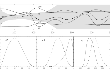
FIG. 4.: Top panel: The total derivative along the degenerate direction (dot-dashed) described in the text is decomposed into variations in four parameters ($\omega_{b}$, $n_{s}$, AD, NIV), which cancel to within the experimental error bars (shaded). Bottom panel: (left) marginalized prior for the adiabatic mode contribution $z_{\mbox{AD}}$, no data; (centre) marginalized posterior for $z_{\mbox{AD}}$ with uniform prior on all models (dashed) and with uniform prior on $z_{\mbox{AD}}$ (solid); (right) marginalized posterior for $\omega_{b}$ with priors as in centre panel.

The greatest impact, however, is on the baryon density distribution, which is significantly broadened, with a median value twice as large as in the adiabatic case. The drastic shift in the baryon density is associated with a flat direction in parameter space, which was observed previously in [9] but not investigated further. Here we clarify the nature of this degeneracy. In Fig. 4 we illustrate how a change in a high-likelihood model $C_{\ell}$ due to a 10% increase in $\omega_{b}$ is compensated by a 40% increase in the power of the pure NIV mode, a 1.4% increase in the value of $n_{s}$ and a 14% decrease in the power of the pure AD mode, to well within the CMB error bars. We have found that there is a high-likelihood plateau connecting the mixed model to the adiabatic model. It is along this plateau that $\omega_{b}$ and $n_{s}$ are shifted to higher values.

We found that the allowed fractional contribution of isocurvature modes depends sensitively on the choice of prior. The problem is that no natural notion of a “uniform” prior stands out, in particular when correlations between the modes are allowed. The prior presented earlier can be argued to be biased against models where a single mode dominates (such as the pure adiabatic model) because such models have a comparatively minuscule phase space density. This “entropy” effect is illustrated in the bottom left hand panel of Fig. 4, where the a posteriori distribution for $z_{\mbox{AD}}$ that would result with no data is plotted. We observe that the pure adiabatic model has zero density solely on account of phase space volume effects. In the bottom centre panel of Fig. 4 we show the posterior distribution for $z_{\mbox{AD}}$ that would result from dividing out this phase space density effect (solid curve), compared to the original posterior (dashed). After the rescaling of the prior, the allowed isocurvature contribution is greatly suppressed. In the bottom right panel of Fig. 4 we see that the reweighted posterior for $\omega_{b}$ overlaps with the conventional value, although much higher values are still allowed.

We have restricted our analysis to flat models and have assigned a single spectral index to all modes. Relaxing either of these restrictions will open up interesting regions of parameter space. However, it is evident from the results presented here that further precision data is required before meaningful constraints can be placed on extended parameter sets. Future high quality CMB polarisation data promises to provide such strong constraints [18], while improved temperature and polarisation spectra from WMAP, the recently available SDSS dataset and higher quality small-scale temperature measurements from ground-based experiments will allow further progress on these issues.

Acknowledgments: MB thanks Mr D. Avery for support through the SW Hawking Fellowship in Mathematical Sciences at Trinity Hall. JD acknowledges a PPARC studentship. PGF thanks the Royal Society. KM acknowledges a PPARC Fellowship and a Natal University research grant. CS is supported by a Leverhulme Foundation grant. We thank R. Durrer, U. Seljak, D. Spergel and R. Trotta for useful discussions.

REFERENCES

- [1] G. Hinshaw et al., Astrophys. J. Supp. 148, 135 (2003). A. Kogut et al., Astrophys. J. Supp. 148, 161 (2003).
- [2] C.L. Kuo, et al., astro-ph/0212289 (2002); J.E. Ruhl et al., Astrophys. J. 599, 786 (2003); T.J Pearson et al., Astrophys. J. 591, 556 (2003); P.F. Scott et al., Mon. Not. R. Astron. Soc. 341, 1076 (2003).
- [3] W. J. Percival et al., Mon. Not. R. Astron. Soc. 327, 1297 (2001).
- [4] M. Tegmark et al., astro-ph/0310725 (2003).
- [5] J. R Bond & G. Efstathiou, Mon. Not. R. Astron. Soc. 22, 33 (1987); P. J. E. Peebles, Nature 327, 210 (1987); Astrophys. J. Lett. Ed. 315, L73 (1987); Astrophys. J. 510, 531 (1999).
- [6] M. Bucher, K. Moodley & N. Turok, Phys. Rev. D. 62, 083508 (2000).
- [7] A. Rebhan & D. Schwarz, Phys. Rev. D 50, 2541 (1994); A. Challinor & A. Lasenby, Astrophys. J. 513, 1 (1999).
- [8] E. Pierpaoli, J. Garcia-Bellido & S. Borgani, J. High. Energy. Phys. 10, 15 (1999); K. Enqvist & H. Kurki-Suonio, Phys. Rev. D 61, 043002 (2000); K. Enqvist, H. Kurki-Suonio & J. Valiviita, Phys. Rev. D 62, 103003 (2000); L. Amendola et al., Phys. Rev. Lett. 88, 211302 (2002); H. V. Peiris et al., Astrophys. J. 148, 213 (2003); C. Gordon & A. Lewis, Phys. Rev. D 67 123513 (2003); J. Valiviita & V. Muhonen, Phys. Rev. Lett. 91, 131302 (2003); P. Crotty et al., Phys. Rev. Lett. 91, 171301 (2003); C. Gordon & K. A. Malik, astro-ph/0311102 (2003).
- [9] R. Trotta, A. Riazuelo & R. Durrer, Phys. Rev. Lett. 87, 231301 (2001); Phys. Rev. D 67, 063520 (2003).
- [10] M. Bucher, K. Moodley & N. Turok, Phys. Rev. D 66, 023528 (2002).
- [11] D. N. Spergel et al., Astrophys. J. 148, 213 (2003).
- [12] M. Kaplinghat, L. Knox & C. Skordis, Astrophys. J. 578, 665 (2002).
- [13] http://www.cmbfast.org/
- [14] K. Moodley et al., in preparation.
- [15] X. Wang et al., Phys. Rev. D 68, 123001 (2003).
- [16] L. Verde et al., Astrophys. J. Suppl. 148, 195 (2003).
- [17] J. A. Peacock et al., Nature 410, 169 (2001).
- [18] M. Bucher, K. Moodley & N. Turok, Phys. Rev. Lett. 87, 191301 (2001).